
Stability of Interval Type-3 Fuzzy Controllers for Autonomous Vehicles


 , ,
, ,  , , ,
, , ,  and
and 
Abstract
:1. Introduction
2. Problem Formulation
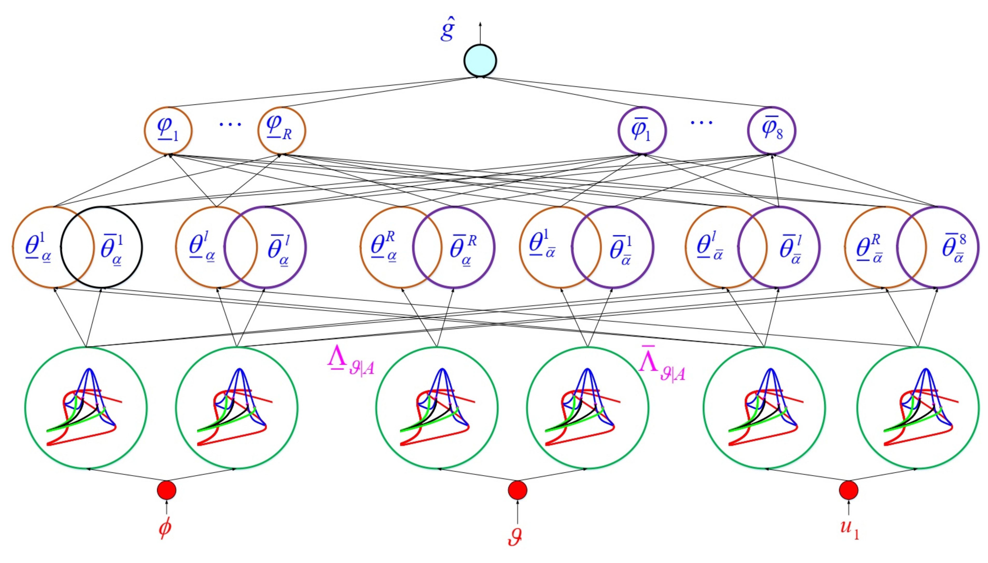
3. Type-3 FLS
- (1)
- The inputs of and are and and the inputs of and are , and .
- (2)
- The suggested membership functions (MFs) are shown in Figure 4. Two MFs are considered for inputs , and . The centers of Gaussian MFs correspond to the upper bound (UB) and lower bound (LB) of inputs. The upper MF is denoted by and the lower MF is denoted by . For , the upper memberships of and for the upper slice and lower slices areSimilarly, the lower memberships are obtained aswhere and are the centers of and , respectively. and are the upper width of at upper slice and lower slices . For input , we haveSimilarly, the lower memberships are obtained aswhere and are the centers of and , respectively. and are the upper width of at upper slice and lower slices .
- (3)
- The output of is written aswhere and arewhere R is the rule numbers, and represent the rule parameters. and arewhere denotes slices numbers andwhere the rule is given as
4. Main Reults
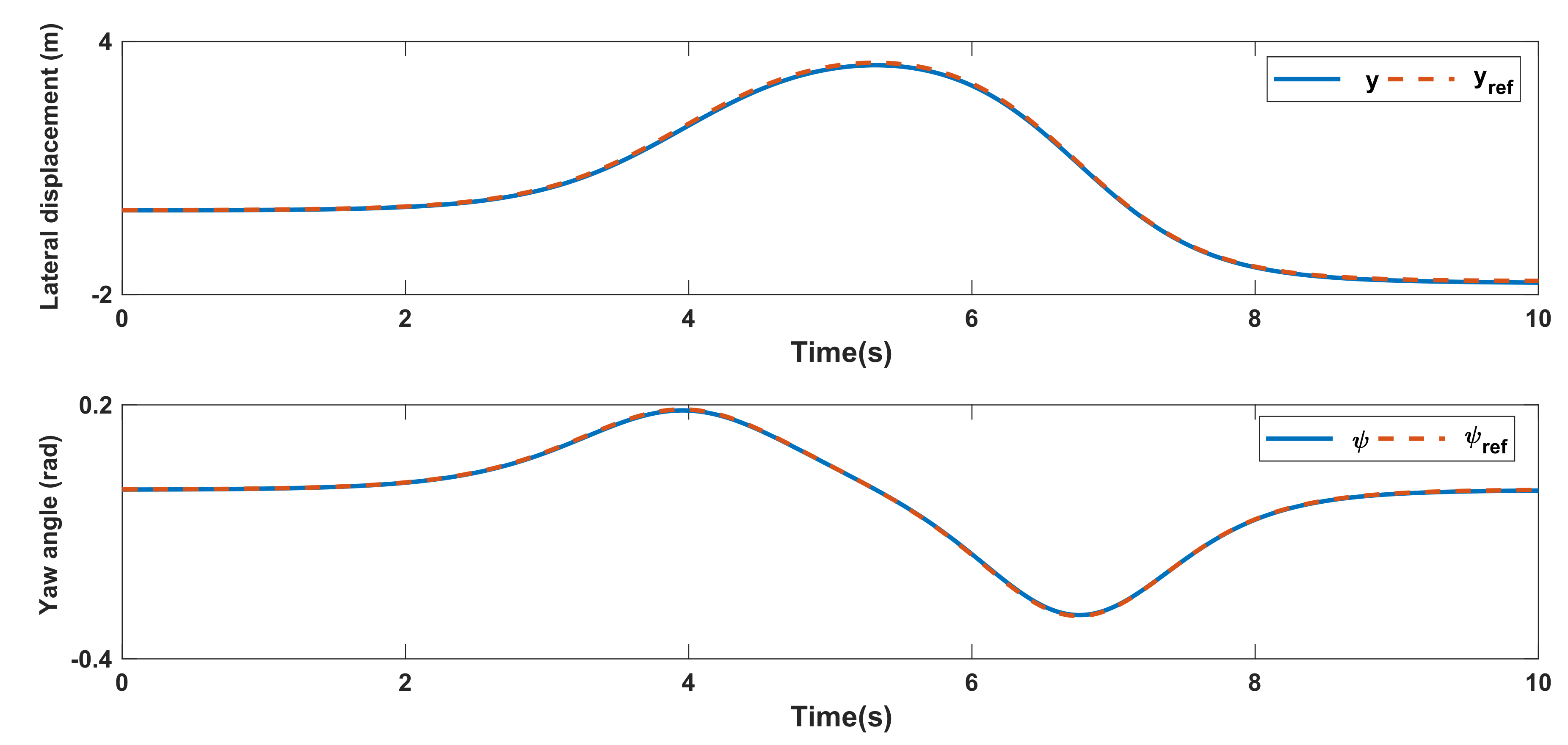
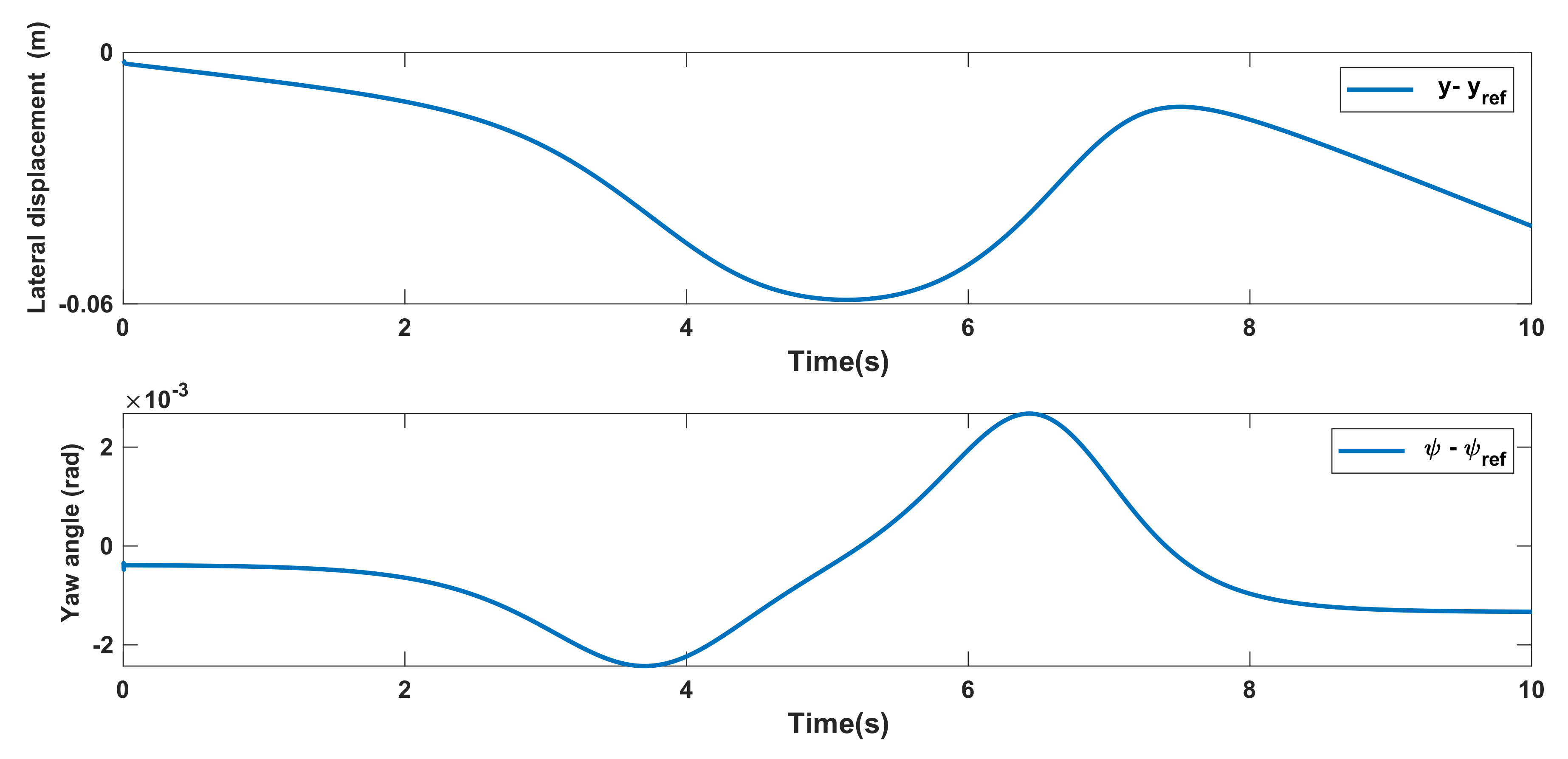
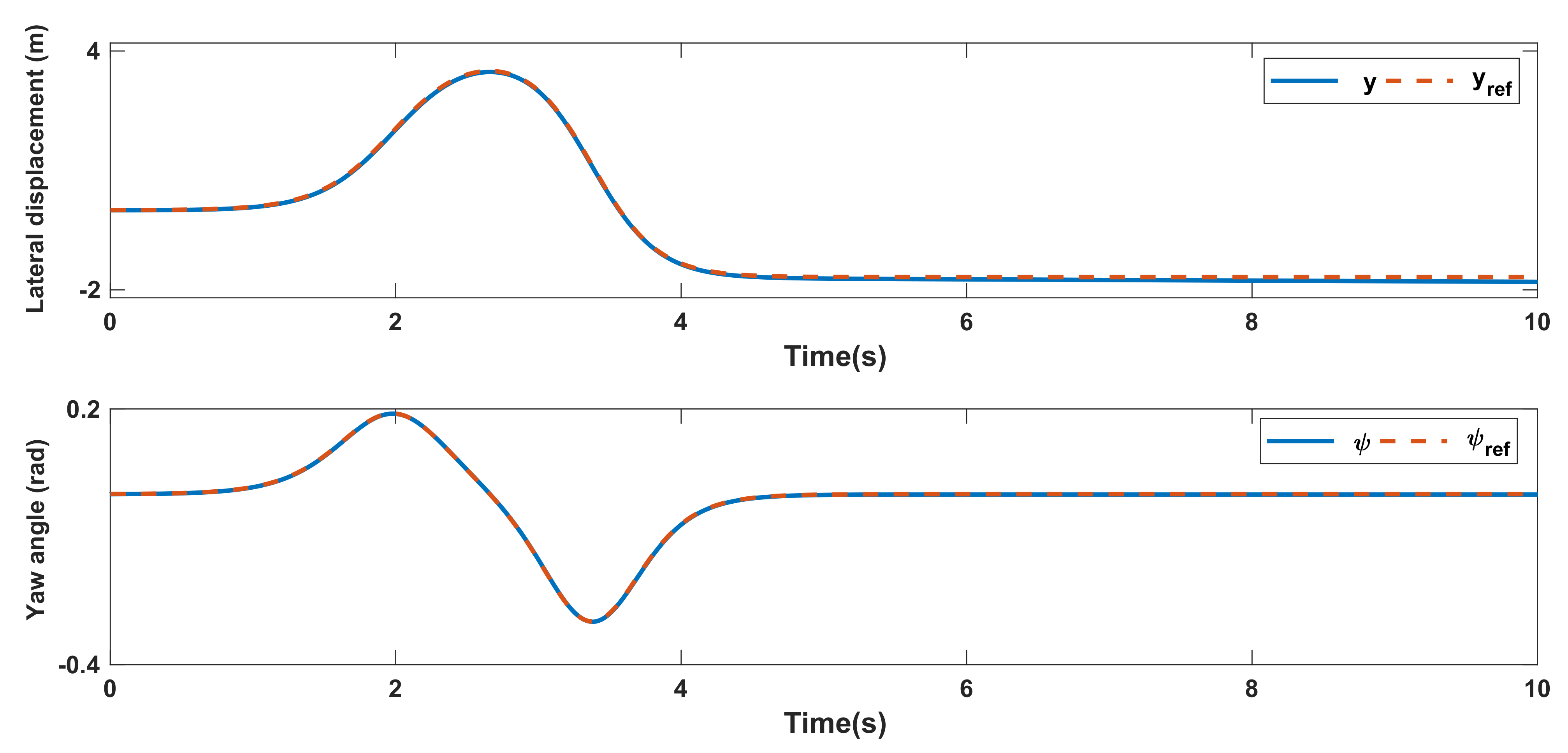
5. Simulations
5.1. Effect of Longitudinal Velocity
5.2. Effect of Disturbances
6. Conclusions
Author Contributions
Funding
Institutional Review Board Statement
Informed Consent Statement
Data Availability Statement
Acknowledgments
Conflicts of Interest
References
- Jin, X.; Yang, J.; Li, Y.; Zhu, B.; Wang, J.; Yin, G. Online estimation of inertial parameter for lightweight electric vehicle using dual unscented Kalman filter approach. IET Intell. Transp. Syst. 2020, 14, 412–422. [Google Scholar] [CrossRef]
- Tian, M.W.; Talebizadehsardari, P. Energy cost and efficiency analysis of building resilience against power outage by shared parking station for electric vehicles and demand response program. Energy 2021, 215, 119058. [Google Scholar] [CrossRef]
- Jin, X.; Wang, J.; Sun, S.; Li, S.; Yang, J.; Yan, Z. Design of constrained robust controller for active suspension of in-wheel-drive electric vehicles. Mathematics 2021, 9, 249. [Google Scholar] [CrossRef]
- Chen, C.H.; Jeng, S.Y.; Lin, C.J. Mobile robot wall-following control using fuzzy logic controller with improved differential search and reinforcement learning. Mathematics 2020, 8, 1254. [Google Scholar] [CrossRef]
- Chen, C.H.; Jeng, S.Y.; Lin, C.J. Using an Adaptive Fuzzy Neural Network Based on a Multi-Strategy-Based Artificial Bee Colony for Mobile Robot Control. Mathematics 2020, 8, 1223. [Google Scholar] [CrossRef]
- Nakata, R.; Tanemura, M.; Chida, Y.; Mitsuhashi, T. Undershoot response analysis of circular path-following control of an autonomous vehicle. Mech. Eng. J. 2021, 8, 21-00002. [Google Scholar] [CrossRef]
- Liang, X.; Qu, X.; Hou, Y.; Li, Y.; Zhang, R. Finite-time unknown observer based coordinated path-following control of unmanned underwater vehicles. J. Frankl. Inst. 2021, 358, 2703–2721. [Google Scholar] [CrossRef]
- Huang, C.; Zhang, X.; Zhang, G. Decentralized event-triggered cooperative path-following control for multiple autonomous surface vessels under actuator failures. Appl. Ocean Res. 2021, 113, 102751. [Google Scholar] [CrossRef]
- Qu, X.; Liang, X.; Hou, Y.; Li, Y.; Zhang, R. Path-following control of unmanned surface vehicles with unknown dynamics and unmeasured velocities. J. Mar. Sci. Technol. 2021, 26, 395–407. [Google Scholar] [CrossRef]
- Wang, S.; Levin, M.W.; Caverly, R.J. Optimal parking management of connected autonomous vehicles: A control-theoretic approach. Transp. Res. Part C Emerg. Technol. 2021, 124, 102924. [Google Scholar] [CrossRef]
- Yoon, Y.; Kim, C.; Lee, J.; Yi, K. Interaction-Aware Probabilistic Trajectory Prediction of Cut-In Vehicles Using Gaussian Process for Proactive Control of Autonomous Vehicles. IEEE Access 2021, 9, 63440–63455. [Google Scholar] [CrossRef]
- Huang, J.; Wang, W.; Su, X. Adaptive iterative learning control of multiple autonomous vehicles with a time-varying reference under actuator faults. IEEE Trans. Neural Netw. Learn. Syst. 2021, 1–14. [Google Scholar] [CrossRef]
- Xiao, W.; Cassandras, C.G.; Belta, C.A. Bridging the gap between optimal trajectory planning and safety-critical control with applications to autonomous vehicles. Automatica 2021, 129, 109592. [Google Scholar] [CrossRef]
- Zhao, B.; Zhang, X.; Liang, C. A novel path-following control algorithm for surface vessels based on global course constraint and nonlinear feedback technology. Appl. Ocean Res. 2021, 111, 102635. [Google Scholar] [CrossRef]
- Cao, X.; Tian, Y.; Ji, X.; Qiu, B. Fault-Tolerant Controller Design for Path Following of the Autonomous Vehicle under the Faults in Braking Actuators. IEEE Trans. Transp. Electrif. 2021, 7, 2530–2540. [Google Scholar] [CrossRef]
- Sanchez, I.; D’Jorge, A.; Raffo, G.V.; González, A.H.; Ferramosca, A. Nonlinear Model Predictive Path Following Controller with Obstacle Avoidance. J. Intell. Robot. Syst. 2021, 102, 1–18. [Google Scholar] [CrossRef]
- Holovatenko, I.; Pysarenko, A. Energy-Efficient Path-Following Control System of Automated Guided Vehicles. J. Control Autom. Electr. Syst. 2021, 32, 390–403. [Google Scholar] [CrossRef]
- Xie, J.; Xu, X.; Wang, F.; Tang, Z.; Chen, L. Coordinated control based path following of distributed drive autonomous electric vehicles with yaw-moment control. Control Eng. Pract. 2021, 106, 104659. [Google Scholar] [CrossRef]
- Yañez-Badillo, H.; Tapia-Olvera, R.; Beltran-Carbajal, F. Adaptive Neural Motion Control of a Quadrotor UAV. Vehicles 2020, 2, 468–490. [Google Scholar] [CrossRef]
- Yañez-Badillo, H.; Beltran-Carbajal, F.; Tapia-Olvera, R.; Favela-Contreras, A.; Sotelo, C.; Sotelo, D. Adaptive Robust Motion Control of Quadrotor Systems Using Artificial Neural Networks and Particle Swarm Optimization. Mathematics 2021, 9, 2367. [Google Scholar] [CrossRef]
- Napole, C.; Barambones, O.; Calvo, I.; Derbeli, M.; Silaa, M.Y.; Velasco, J. Advances in Tracking Control for Piezoelectric Actuators Using Fuzzy Logic and Hammerstein-Wiener Compensation. Mathematics 2020, 8, 2071. [Google Scholar] [CrossRef]
- Tian, M.; Yan, S.; Tian, X. Discrete approximate iterative method for fuzzy investment portfolio based on transaction cost threshold constraint. Open Phys. 2019, 17, 41–47. [Google Scholar] [CrossRef]
- Derbeli, M.; Napole, C.; Barambones, O. Machine Learning Approach for Modeling and Control of a Commercial Heliocentris FC50 PEM Fuel Cell System. Mathematics 2021, 9, 2068. [Google Scholar] [CrossRef]
- Napole, C.; Derbeli, M.; Barambones, O. Fuzzy Logic Approach for Maximum Power Point Tracking Implemented in a Real Time Photovoltaic System. Appl. Sci. 2021, 11, 5927. [Google Scholar] [CrossRef]
- Tork, N.; Amirkhani, A.; Shokouhi, S.B. An adaptive modified neural lateral-longitudinal control system for path following of autonomous vehicles. Eng. Sci. Technol. Int. J. 2021, 24, 126–137. [Google Scholar]
- Wang, M.; Chen, J.; Deng, Z.; Xiang, Y. Velocity Planning Method Base on Fuzzy Neural Network for Autonomous Vehicle. IEEE Access 2021, 9, 19111–19126. [Google Scholar] [CrossRef]
- Yang, Z.; Huang, J.; Yang, D.; Zhong, Z. Design and Optimization of Robust Path Tracking Control for Autonomous Vehicles with Fuzzy Uncertainty. IEEE Trans. Fuzzy Syst. 2021, 1. [Google Scholar] [CrossRef]
- Li, M.; Long, Y.; Li, T.; Bai, W. Observer-Based Adaptive Fuzzy Event-Triggered Path Following Control of Marine Surface Vessel. Int. J. Fuzzy Syst. 2021, 23, 2021–2036. [Google Scholar] [CrossRef]
- Lin, F.; Wang, S.; Zhao, Y.; Cai, Y. Research on autonomous vehicle path tracking control considering roll stability. Proc. Inst. Mech. Eng. Part D J. Automob. Eng. 2021, 235, 199–210. [Google Scholar] [CrossRef]
- Wu, Q.; Cheng, S.; Li, L.; Yang, F.; Meng, L.J.; Fan, Z.X.; Liang, H.W. A fuzzy-inference-based reinforcement learning method of overtaking decision making for automated vehicles. Proc. Inst. Mech. Eng. Part D J. Automob. Eng. 2021, 09544070211018099. [Google Scholar] [CrossRef]
- Wei, L.; Wang, X.; Li, L.; Fan, Z.; Dou, R.; Lin, J. TS fuzzy model predictive control for vehicle yaw stability in nonlinear region. IEEE Trans. Veh. Technol. 2021, 70, 7536–7546. [Google Scholar] [CrossRef]
- Xu, X.; Su, P.; Wang, F.; Chen, L.; Xie, J.; Atindana, V.A. Coordinated control of dual-motor using the interval type-2 fuzzy logic in autonomous steering system of AGV. Int. J. Fuzzy Syst. 2021, 23, 1070–1086. [Google Scholar] [CrossRef]
- Mohammadzadeh, A.; Taghavifar, H. A robust fuzzy control approach for path-following control of autonomous vehicles. Soft Comput. 2020, 24, 3223–3235. [Google Scholar] [CrossRef]
- Yao, L.; Pitla, S.K.; Zhao, C.; Liew, C.; Hu, D.; Yang, Z. An Improved Fuzzy Logic Control Method for Path Tracking of an Autonomous Vehicle. Trans. ASABE 2020, 63, 1895–1904. [Google Scholar] [CrossRef]
- Nabipour, N.; Qasem, S.N.; Jermsittiparsert, K. Type-3 fuzzy voltage management in PV/hydrogen fuel cell/battery hybrid systems. Int. J. Hydrog. Energy 2020, 45, 32478–32492. [Google Scholar] [CrossRef]
- Liu, Z.; Mohammadzadeh, A.; Turabieh, H.; Mafarja, M.; Band, S.S.; Mosavi, A. A New Online Learned Interval Type-3 Fuzzy Control System for Solar Energy Management Systems. IEEE Access 2021, 9, 10498–10508. [Google Scholar] [CrossRef]
- Ma, C.; Mohammadzadeh, A.; Turabieh, H.; Mafarja, M.; Band, S.S.; Mosavi, A. Optimal Type-3 Fuzzy System for Solving Singular Multi-Pantograph Equations. IEEE Access 2020, 8, 225692–225702. [Google Scholar] [CrossRef]
- Vafaie, R.H.; Mohammadzadeh, A.; Piran, M. A new type-3 fuzzy predictive controller for MEMS gyroscopes. Nonlinear Dyn. 2021, 106, 381–403. [Google Scholar] [CrossRef]
- Cao, Y.; Raise, A.; Mohammadzadeh, A.; Rathinasamy, S.; Band, S.S.; Mosavi, A. Deep learned recurrent type-3 fuzzy system: Application for renewable energy modeling/prediction. Energy Rep. 2021, in press. [Google Scholar] [CrossRef]
- Mohammadzadeh, A.; Sabzalian, M.H.; Zhang, W. An interval type-3 fuzzy system and a new online fractional-order learning algorithm: Theory and practice. IEEE Trans. Fuzzy Syst. 2019, 28, 1940–1950. [Google Scholar] [CrossRef]
- Falcone, P.; Borrelli, F.; Asgari, J.; Tseng, H.E.; Hrovat, D. Predictive active steering control for autonomous vehicle systems. IEEE Trans. Control Syst. Technol. 2007, 15, 566–580. [Google Scholar] [CrossRef]
- Xia, Y.; Pu, F.; Li, S.; Gao, Y. Lateral path tracking control of autonomous land vehicle based on ADRC and differential flatness. IEEE Trans. Ind. Electron. 2016, 63, 3091–3099. [Google Scholar] [CrossRef]
- Hwang, C.-L.; Yang, C.-C.; Hung, J.Y. Path Tracking of an Autonomous Ground Vehicle with Different Payloads by Hierarchical Improved Fuzzy Dynamic Sliding-Mode Control. IEEE Trans. Fuzzy Syst. 2018, 26, 899–914. [Google Scholar] [CrossRef]


| Parameter | Value | Unit |
|---|---|---|
| 67,600 | N/rad | |
| 2352 | kg m2 | |
| 1.64 | m | |
| 1.04 | m | |
| 47,600 | N/rad | |
| m | 1481 | kg |
| ADRC [42] | LQT [42] | T2FLC [33] | FLS-MPC [43] | Proposed | |
|---|---|---|---|---|---|
| y | 0.2207 | 1.1049 | 0.0268 | 0.0250 | 0.0241 |
| Maximum of | 0.5592 | 1.7757 | 0.0451 | 0.0432 | 0.0317 |
| 0.0178 | 0.0592 | 0.0014 | 0.0015 | 1.2 × 10⁻⁴ | |
| Maximum of | 0.0363 | 0.1456 | 0.0017 | 0.0015 | 1.2 × 10⁻⁴ |
| 10 m/s | 20 m/s | 30 m/s | |
|---|---|---|---|
| y | 0.0241 | 0.0338 | 0.0413 |
| Maximum of | 0.0317 | 0.0498 | 0.0531 |
| 1.2 × 10⁻⁴ | 1.3 × 10 | 1.3 × 10⁻⁴ | |
| Maximum of | 1.1 × 10⁻⁴ | 1.5 × 10⁻⁴ | 1.7 × 10⁻⁴ |
| case 1: | Changes of / as |
| case 2: | Changes of / as |
| case 3: | A pulse signal at time 2.5 s with width 0.25 |
| Normal | Case 1 | Case 2 | Case 3 | |
|---|---|---|---|---|
| y | 0.0338 | 0.0339 | 0.0341 | 0.0343 |
| Maximum of | 0.0317 | 0.0401 | 0.0451 | 0.0527 |
| 1.30 × 10⁻⁴> | 1.32 × 10⁻⁴ | 1.41 × 10⁻⁴ | 1.47 × 10⁻⁴ | |
| Maximum of | 1.50 × 10⁻⁴ | 1.53 × 10⁻⁴ | 1.61 × 10⁻⁴ | 1.66 × 10⁻⁴ |
Publisher’s Note: MDPI stays neutral with regard to jurisdictional claims in published maps and institutional affiliations. |
© 2021 by the authors. Licensee MDPI, Basel, Switzerland. This article is an open access article distributed under the terms and conditions of the Creative Commons Attribution (CC BY) license (https://creativecommons.org/licenses/by/4.0/).
Share and Cite
Tian, M.-W.; Yan, S.-R.; Mohammadzadeh, A.; Tavoosi, J.; Mobayen, S.; Safdar, R.; Assawinchaichote, W.; Vu, M.T.; Zhilenkov, A. Stability of Interval Type-3 Fuzzy Controllers for Autonomous Vehicles. Mathematics 2021, 9, 2742. https://doi.org/10.3390/math9212742
Tian M-W, Yan S-R, Mohammadzadeh A, Tavoosi J, Mobayen S, Safdar R, Assawinchaichote W, Vu MT, Zhilenkov A. Stability of Interval Type-3 Fuzzy Controllers for Autonomous Vehicles. Mathematics. 2021; 9(21):2742. https://doi.org/10.3390/math9212742
Chicago/Turabian StyleTian, Man-Wen, Shu-Rong Yan, Ardashir Mohammadzadeh, Jafar Tavoosi, Saleh Mobayen, Rabia Safdar, Wudhichai Assawinchaichote, Mai The Vu, and Anton Zhilenkov. 2021. "Stability of Interval Type-3 Fuzzy Controllers for Autonomous Vehicles" Mathematics 9, no. 21: 2742. https://doi.org/10.3390/math9212742