Abstract
The approximation of curvilinear profiles is very popular for processing digital images and leads to numerous applications such as image segmentation, compression and recognition. In this paper, we develop a novel semi-automatic method based on quasi-interpolation. The method consists of three steps: a preprocessing step exploiting an edge detection algorithm; a splitting procedure to break the just-obtained set of edge points into smaller subsets; and a final step involving the use of a local curve approximation, the Weighted Quasi Interpolant Spline Approximation (wQISA), chosen for its robustness to data perturbation. The proposed method builds a sequence of polynomial spline curves, connected in correspondence of cusps, otherwise. To curb underfitting and overfitting, the computation of local approximations exploits the supervised learning paradigm. The effectiveness of the method is shown with simulation on real images from various application domains.
1. Introduction
Approximating curvilinear profiles in digital images with piecewise polynomials is very attractive in many application domains, as it leads to more compact and less wiggly representations of borders and contours. In this work, we study the applicability of the quasi-interpolation paradigm for approximating open and closed curves that can be modeled as 1-manifolds, that is, topological spaces wherein each point has a neighborhood that is homeomorphic to the Euclidean space of dimension 1; an extension to piecewise 1-manifolds is straightforward by decomposing the curve in 1-manifolds and proceeding one segment at a time [1].
The term quasi-interpolation has been interpreted differently by different authors, depending on the context of application. We here call quasi-interpolant any linear operator L of the form:
where is a function being approximated, are linear functionals, are functions at our disposal (see, for example [2,3]). The coefficients (f) are, in general, one of the following types: linear combinations of given values of the function f to be approximated (discrete type); linear combinations of values of derivatives of f, of order at most d (differential type); linear combinations of weighted mean values of f (integral type). Equation (1) can be interpreted as a “reconstruction” formula: given some input data sampled from the true function f, it creates a tentative reconstruction .
The origin of quasi-interpolation is traditionally traced back to Bernstein’s approximation [4], where the functions are Bernstein polynomials. A rather simple generalization, known as Variation Diminishing Spline Approximation (VDSA), generalizes this construction to B-splines (see, for example [5,6]). Since its inception, quasi-interpolation has been studied to obtain methods that apply to different domains and with the aim of increasing the order of convergence: recent developments include univariate and tensor-product spaces [7,8,9], triangular meshes [10,11,12,13], quadrangulations [14] and tetrahedra partitions [15], among others.
Unlike traditional quasi interpolation spline methods, which generally focus on the approximation of functions with strong regularity conditions, Weighted Quasi Interpolant Spline Approximations (wQISAs) [16,17] aims to provide local approximations of point clouds which can be affected by artifacts such as noise and outliers. However, a paradigm to compute global approximations was, so far, missing; indeed, the only two global approximations presented in [16] are obtained by manually processing the set of edge points, thanks to the quite simple geometry of the studied profiles. In this paper, we introduce a novel method that exploits wQISAs to construct global approximations of planar curvilinear profiles, with application to digital image processing. More specifically, the main contributions of this paper are:
- The introduction of a novel algorithm, based on Weighted Quasi-Interpolant Spline Approximations, to compute global approximations of planar curvilinear profiles;
- The validation of the method on real images from different application domains with respect to different evaluation measures.
The smoothness of a curve is generally distinguished between parametric continuity and geometric continuity [18,19]. A curve is said to be continuous at if it is continuous at and if the first n left and right derivatives of match at , that is,
A curve is said to be continuous at if, up to regular re-parametrization, it is continuous at . Recently, the concept of fractional continuity has been proposed for generalized fractional Bézier curves [20]. In our context, the global approximation of a planar profile is computed by gluing together local approximations, by imposing a continuity in correspondence of cusps, and a continuity otherwise; while it is possible to consider the more general case of (or ) continuity, continuity has proved to be sufficient in many practical applications (see, for example [21,22]).
The remainder of the paper is organized as follows. In Section 2, we provide some notation and background knowledge about the wQISA family. In Section 3, the core of our paper, we introduce our reconstruction algorithm. To test the validity of the suggested approach, Section 4 presents several experimental results on images from different application domains and with respect to different evaluation measures. Concluding remarks end the paper.
2. Preliminary Concepts
This section is meant to list some basic definitions regarding the wQISA family, as well as to introduce the essential terminology and notation. Because in this paper we focus on 1-manifolds, we restrict our attention to a univariate formulation of wQISA; for more details on the more general multivariate setting and an extended analysis of the theoretical properties, we refer the reader to [16].
Given a degree p, a knot vector is said to be -regular if no knot occurs more than times and each boundary knot occurs exactly times.
Let be a point cloud and . Let be a -regular knot vector with boundary knots and . A Weighted Quasi Interpolant Spline Approximation of degree p to the point cloud over the knot vector is defined by:
where are the knot averages, the expression,
gives the control polygon estimator with weight function ; denotes the B-spline of degree p, which is uniquely determined by the local knot vector . Note that, given a point cloud, its wQISA depends on the following inputs: a spline space, uniquely defined by a degree and a (global) knot vector, and a weight function (possibly, with free parameters to be tuned). An example of weight function is given by the k-Nearest Neighbours (k-NN) average:
where ; denotes the neighborhood of u defined by the k closest points of the point cloud; here, k is the free parameter.
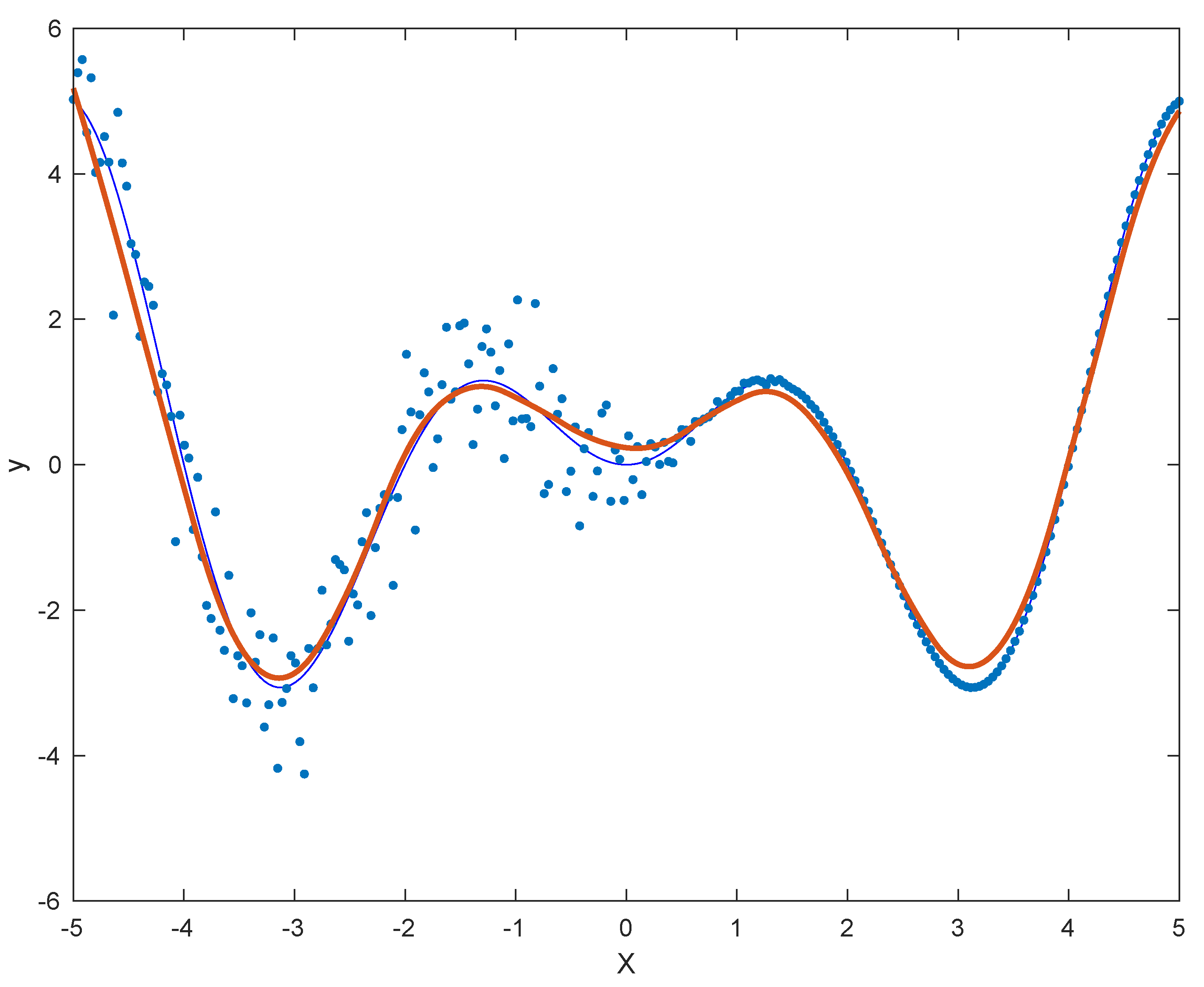
Figure 1 shows the approximation of a dataset of 250 points when a 5-NN weight is considered. The point cloud is sampled from the analytic function , and is eventually perturbed with Gaussian noise , where
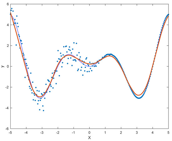
Figure 1.
Variable noise approximation. The analytic function is sampled and then perturbed with (non-uniform) Gaussian noise of mean 0 and the standard deviation of Equation (5). The resulting wQISA approximation, obtained by a 5-NN weight function, is displayed red.
The approximation is computed by a quadratic spline space containing B-splines over a uniform knot vector.
3. Curvilinear Profile Approximation via a Quasi-Interpolation-Based Technique
In this section, we design an algorithm that piecewisely applies wQISA to the approximation and recognition of open and closed planar curvilinear profiles. The method consists of three main steps:
- Pre-processing step (see Section 3.1);
- Point cloud split (see Section 3.2);
- Local approximation via wQISA (see Section 3.3).
3.1. Pre-Processing Step
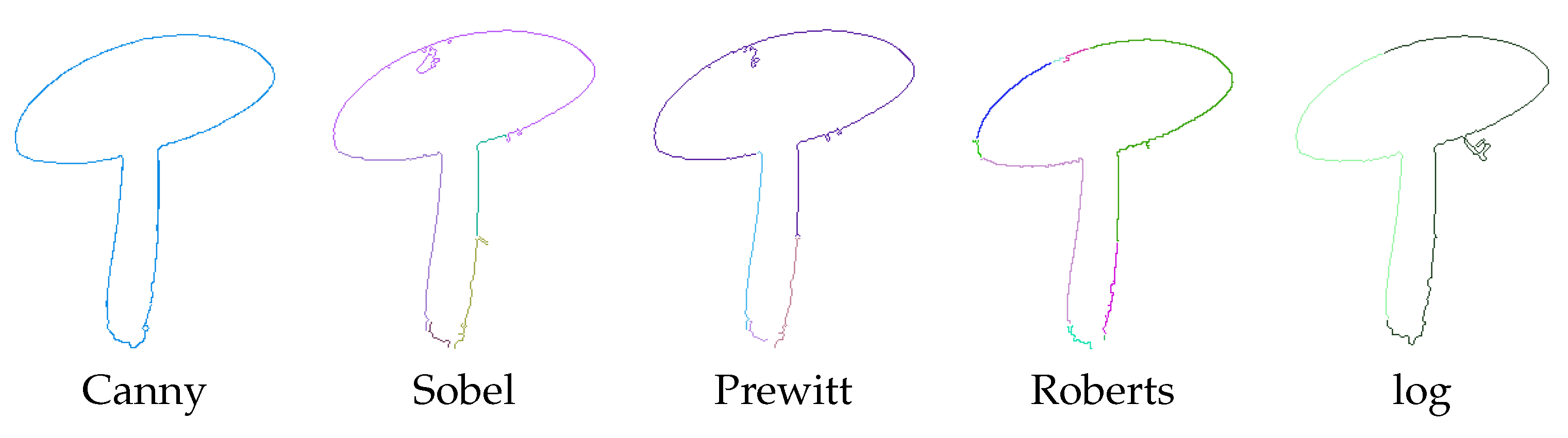
Firstly, we run an edge detection algorithm to an input a (grayscale) image, hereinafter denoted by I: in our case, we used the Canny edge detection [23], as it is considered among the most effective edge detection techniques [24,25]. To give an example, when considering the mushroom of Figure 2, we note that the Canny edge detection algorithm provides a much better result than other popular methods, see Figure 2: indeed, the Canny edge detection provides a much cleaner set of edge points, and is the only one able to identify the whole curvilinear profile without wrongly decomposing it into subparts.
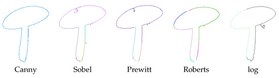
Figure 2.
Different edge detection methods applied to an image presented in Section 4. Different colors identify different 8-connected components.
The pixels identified as discontinuity points by the edge detection algorithm are then processed to identify 8-connected components. Their centres are maintained in . For the sake of conciseness, we will hereinafter suppose that consists of a single 8-connected component; in case of more than one 8-connected component, the reconstruction method will be applied as many times as their number.
For every point in , the local discrete tangent vector is computed (for example, by means of regionprops in MATLAB). All those points with a sharp change in the unit tangent vector are stored in , and will be eventually used to impose a continuity instead of continuity; to put it another way, the order of continuity will be only in correspondence with the identified cusps, as expected. A graphical illustration of the and continuities is given in Figure 3.
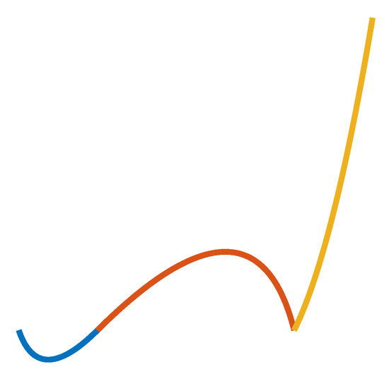
Figure 3.
Graphical illustration of the and continuities: the curves in blue and red are connected with continuity; the curves in red and yellow are connected with continuity.
3.2. Point Cloud Split
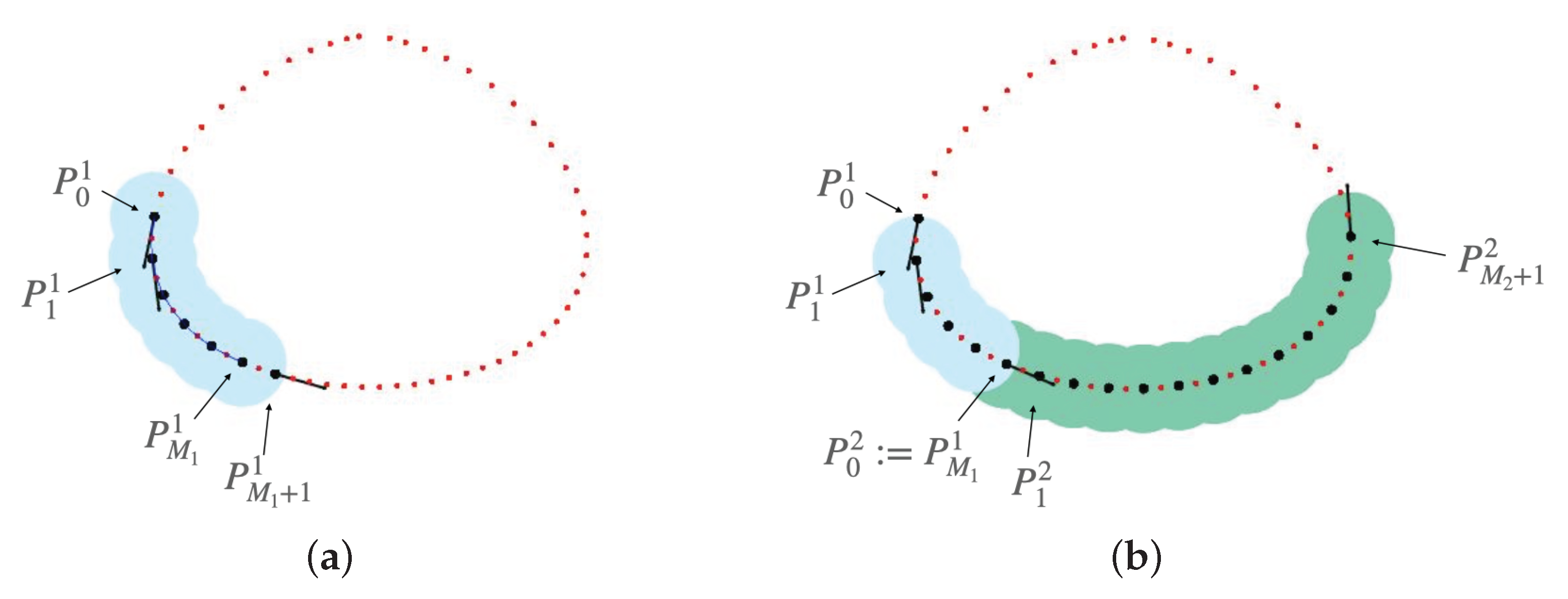
Differently from the method in [26] that iteratively covered a curvilinear profile with disks of fixed radius, in our pipeline the point cloud is split into subsets, each of which is meant to be approximated independently. The key idea behind our procedure is loosely inspired by the concept of tubular neighborhoods—see, for example [27]. A graphical illustration of two possible iterations is given in Figure 4.
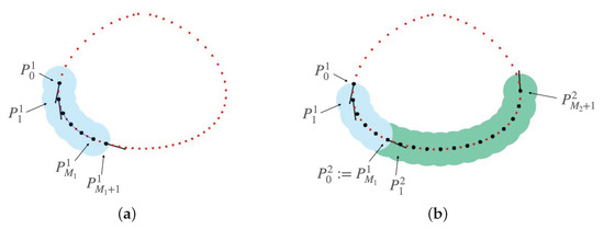
Figure 4.
Graphical illustration for the computation of local tubular neighbourhoods for two iterations of the algorithm. For the sake of clarity, we here consider an over-simplified situation, with a noise-free point cloud represented in red. (a) First iteration; (b) Second iteration.
3.2.1. Constructing the k-th Local Tubular Neighborhood,
Given an initial point , where , and an input radius , let denote the (2-)ball of center and radius . We build a sequence of points such that:
- For any index , the point is computed from as follows:
- –
- Advance step. Set to be the farthest point from in , among all those points that were not contained in any previously-computed balls.
- –
- Smoothing step. Set to be the point in which is the closest to the barycenter of the points in , where is an input value that should account for the amount of noise.
- The index is the first one for which either of the following criteria holds true:
- –
- Angle criterion. The angle between the tangent vectors in and is above the threshold .
- –
- Point criterion. The ball does not contain new points (i.e., points which were not contained in previously-computed balls).
- –
- Loop criterion. The ball contains the initial point .
When stopping because of the angle criterion, we define the k-th local tubular neighbourhood as:
Its candidate edge points are and ; finally, we set to be the initial point for the subsequent local tubular neighborhood. On the contrary, when stopping because of either the point or loop criteria, the k-th local tubular neighbourhood is defined as:
and its candidate edge points are and , where in case the loop criterion holds.
When stopping because of the point criterion, a new search is conducted from the initial point backward, to take into account the possibility of open profiles.
Note that the whole splitting procedure merely relies on the following input: the initial point , the radii and , and the threshold . A more detailed discussion on the parameter setting is left to Section 3.4.
3.2.2. Updating the k-th Local Tubular Neighborhood,
The local tubular neighbourhoods allow us to locally represent the curvilinear profile of interest. However, their construction does not take into account the points in , that is, the points having a sharp change in the tangent vector.
Suppose that a cusp is inside the two balls and . Then, we split the k-th local tubular neighbourhood into two new local tubular neighbourhoods:
- One will contain all balls , plus the reduced ball
- The other one will contain all balls —and , in case of Equation (7)—plus the reduced ball
The cusp will be set to be a common edge point of the two new local tubular neighbourhoods.
3.3. Local Approximation via wQISA
For any , the local parametrization is computed as follows:
- Change of coordinates. Apply a roto-translation to , so that the line segmentlies on the x-axis. This corresponds to assuming that our local approximation can be locally flattened onto the x-axis without any overlap; note that this assumption relies on the parameter .
- Local spline space. Define as the j-th 3-regular knot vector where:
- For any , and , being the abscissa of the roto-translation of with respect to the map . Note that the map can be chosen so that .
- The knots are uniformly sampled in .
- Local wQISA approximation. Compute a local approximation for by applying Equation (2) with k-NN weight function; note that the parameter k in the weight function does not necessarily equal the index k in the sequence of local tubular neighborhoods.
A discussion on the tuning of the free parameters (i.e., knot vector length and k of the k-NN weight function) is provided in Section 3.4.
Given that for any local tubular neighbourhood, the corresponding knot vector is -regular, the final approximation will be automatically continuous. To impose continuity, we exploit -regularity: the tangents to the curve at the boundaries are determined by its 2nd and (n − 1)th control points; we project the 2nd and th onto the straight lines determined by the tangent vectors. A similar reasoning can be applied to interpolate the left and right derivatives at cusps, up to a multiplicative constant.
3.4. Free Parameters and Tuning
The initial point is set to be the cusp, which is the closest to the lower-left corner. If the profile does not exhibit any cusps, we can consider the point of maximum (or minimum) curvature—the closest to the lower-left corner if more than one exists.
The radii and depend on the profiles and the noise level, and are currently empirically set by the user.
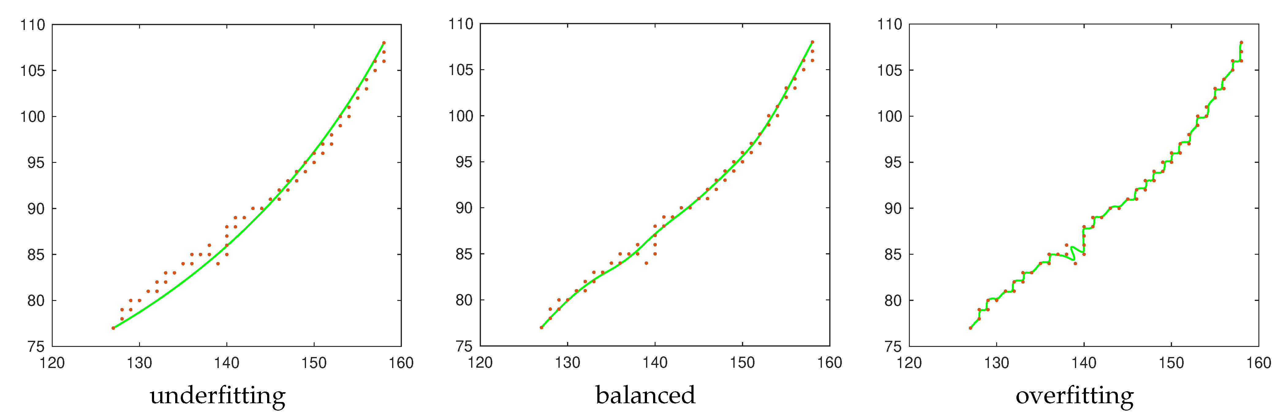
For each local approximation, the optimal global knot vector and the optimal for the weight function can be found by a model assessment and selection procedure, as in statistical learning; more precisely, we proceed by performing Leave-One-Out Cross-Validation (LOO-CV, see [28]), by considering the Root Mean Square Error as a generalization error (see Section 4). This allows us to limit under- and overfitting; an example is given in Figure 5 of a local tubular neighborhood exhibiting both noise and outliers. The use of Cross-Validation for the estimation of the unknown coefficients allows us to interpret the curve fitting problem as a supervised learning problem (see, for example [29]).
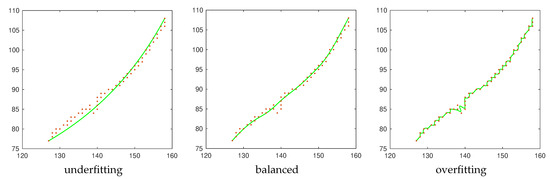
Figure 5.
Three approximations for a local tubular neighborhood from Figure 6. In the left image, the local approximation consists of an oversimplification of the input data. In the right image, the local approximation models the training data too well, resulting in unwanted oscillations that reduce the prediction capability on new points. A good balance between under- and over-fitting is displayed in the central image.
To generalize the method, one could select the continuity at the segment edge points by cross-validation; however, continuity has proved to be sufficient for all the examples given in Section 4.
3.5. Computational Complexity
The computational complexity of the parametrization step is the sum of the single wQISA iterations. On its turn, wQISA mainly depends on the k-NN weight, whose time complexity for estimating a single coefficient is proportional to , where N is the number of points. To further reduce the computational complexity of the k-NN search, we follow the k-d trees approach proposed in [30]. It is worth noting that, each coefficient and each local approximation being computed independently, this task is embarrassingly parallel.
The splitting procedure can itself rely on a k-d tree, thus it has the same computational complexity. On the other hand, it cannot be performed independently, and turns out to be the most demanding part of the algorithm.
4. Experimental Results
We evaluate our method on photographic images, animation images and CT scans. Although the approximation could theoretically make use of B-splines of any degree, we here focus on quadratic spline approximations, as they provide a sufficient flexibility for our purposes; nevertheless, one could consider the degree of each local approximation as an additional parameter to be tuned.
4.1. Performance Measures
To evaluate the quality of an approximation against the input point clouds, the following indicators are considered:
- The Root Mean Square Error (RMSE), that is, the square root of the Mean Square Error, is defined by:being the abscissa of an input point with respect to its local coordinate system, its approximation, and N the cardinality of the input point cloud. Similarly, the Mean Absolute Error (MAE) is given by:
- The (normalized) Directed Hausdorff Distance from the points of to the points of is defined as:where d is the Euclidean distance and L is the diameter of the input point cloud. In our case, we set B to be the input point cloud , while A is given by the points defining our spline approximation.
- The Jaccard index, or Intersection over Union, measures how overlapping two sets A and B are; it is computed as:being the cardinality of a set. The Jaccard index has been intensively applied to measure the performance of curve recognition methods for images (see, for example [31]). Here, we compare the set of pixels corresponding to with the set of pixels crossed by the approximation and their 1-neighbours.
4.2. Photographic Images
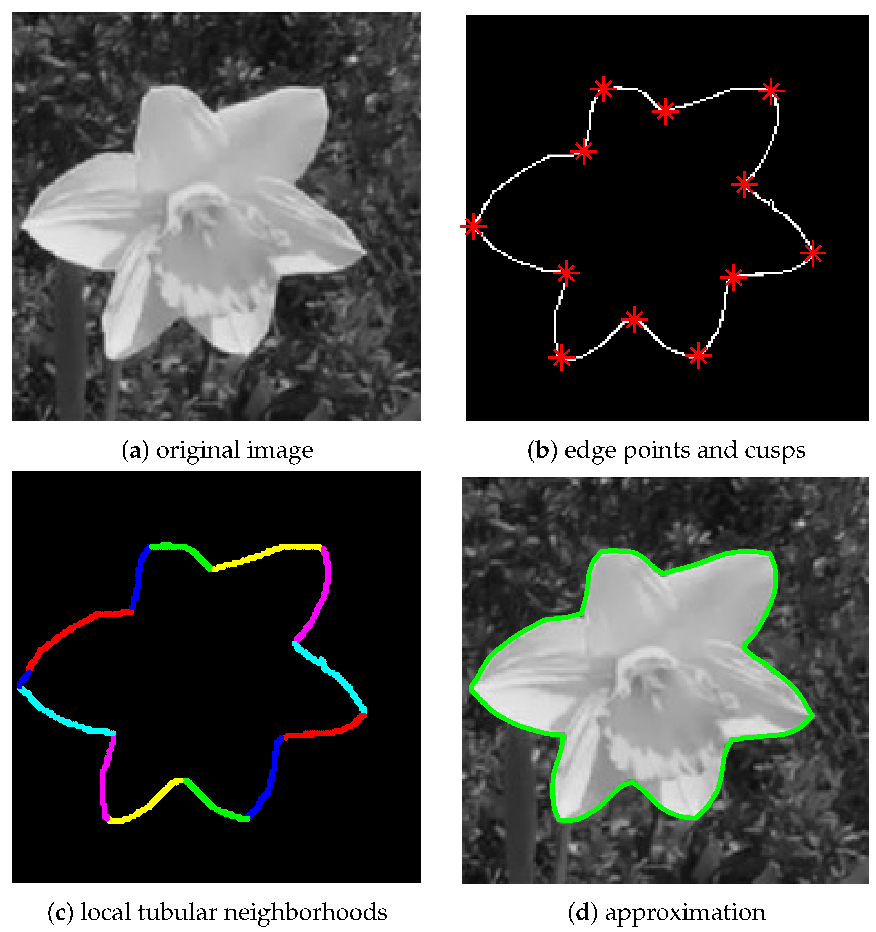
We start by considering a image representing a flower (Image retrieved on MathWorks®), see Figure 6. The use of the Canny edge detection algorithm and the subsequent study of the tangent vector of the profile allows us to identify all cusps, as shown in Figure 6b. The set of edge points is then split into 13 local tubular neighborhoods, see Figure 6c. The obtained approximation, superimposed to the original image, is displayed in Figure 6d. Given that plotting the local tubular neighborhoods is not particularly informative, we just report their number for the remaining examples in Section 4.5.
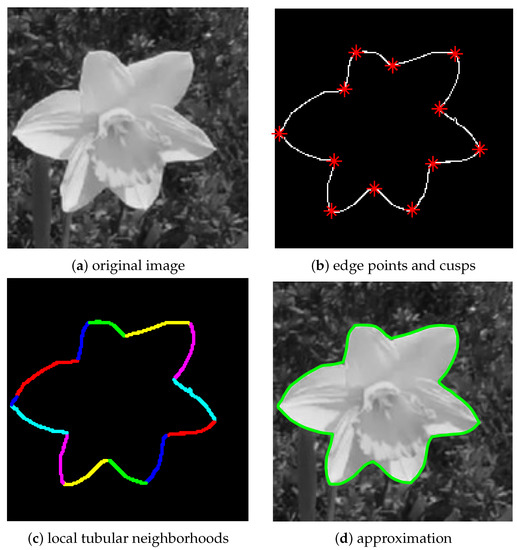
Figure 6.
Recognition and approximation of a daffodil. The input image (a) is pre-processed to obtain the edge points and detect the cusps (b). The point cloud is then split into local segments, see (c). The approximated curve, superimposed to the original image, is given in (d).
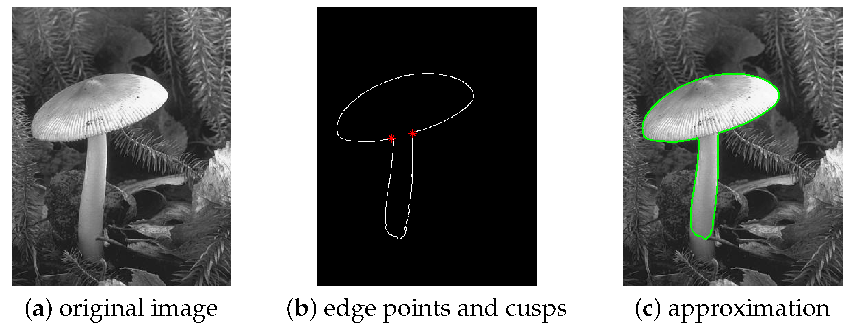
Figure 7 shows a (not surprising) limitation of the method. The edge detection algorithm, applied to the image displayed in Figure 7a, is not able to reveal the whole stalk of the mushroom, see Figure 7b: this results in an accurate approximation of the edge points, as displayed in Figure 7c which is nonetheless missing part of the original object. The image for this test was selected from the Berkeley Segmentation Dataset and Benchmark [32].

Figure 7.
Recognition and approximation of a mushroom. From the original image (a), we extract (b) and approximate the edge points (c).
4.3. Animation Images
A composite example is exhibited in Figure 8. In Figure 8a, the input image is shown. In Figure 8b, some sets of edge points and their cusps are displayed. Different closed and open profiles are approximated and provided in Figure 8c: the circle logo and the letter M therein, the eyebrows and the moustache. Note that all profiles have cusps.
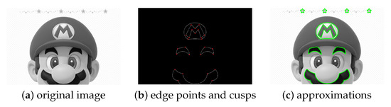
Figure 8.
Recognition and approximation of different profiles in Super Mario. From the original image (a), we extract (b) and approximate the circle logo and the letter M therein, the eyebrows and the moustache (c).
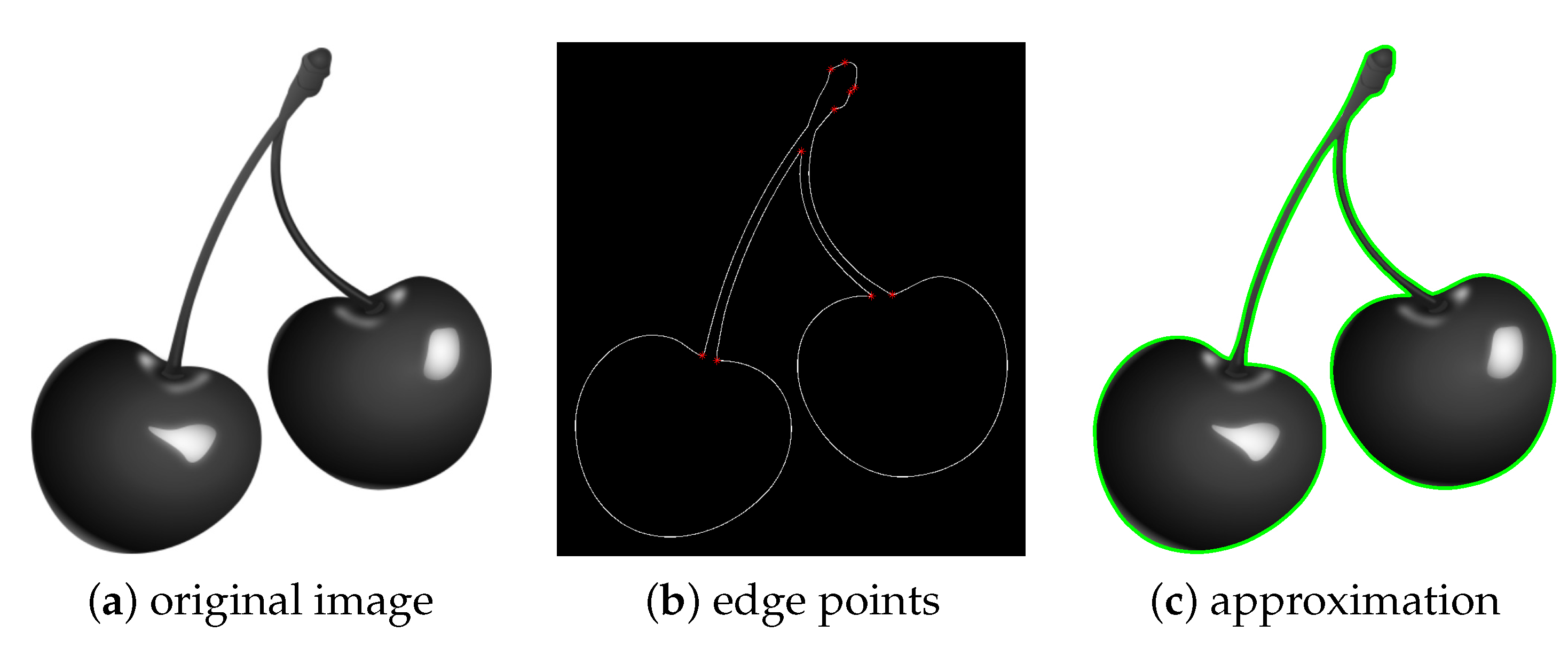
A single but more complex closed profile is provided in the image from Figure 9a, obtained from the dataset used in [33]. The set of edge points and the detected cusps are given in Figure 9b, while the final approximation is shown in Figure 9c.
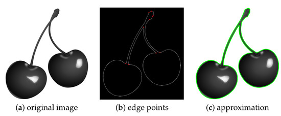
Figure 9.
Recognition and approximation of a cherry profile. From the original image (a), we extract the edge points and identify cusps (b), and produce the final approximation given in (c).
4.4. Medical Images
Figure 10 presents the study undertaken on the CT image of a head (Image retrieved on https://vtk.org, accessed on 1 September 2021). For the external profile in Figure 10a, the set of edge points Figure 10b does not exhibit any cusps. The approximation, superimposed to the original image in Figure 10c, shows an overall satisfying result.
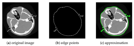
Figure 10.
Recognition and approximation of the external profile of a human head. The original image (a) is treated to obtain the edge points (b), which do not contain cusps in this case; the approximation of the external profile, superimposed to the image, is given in (c).
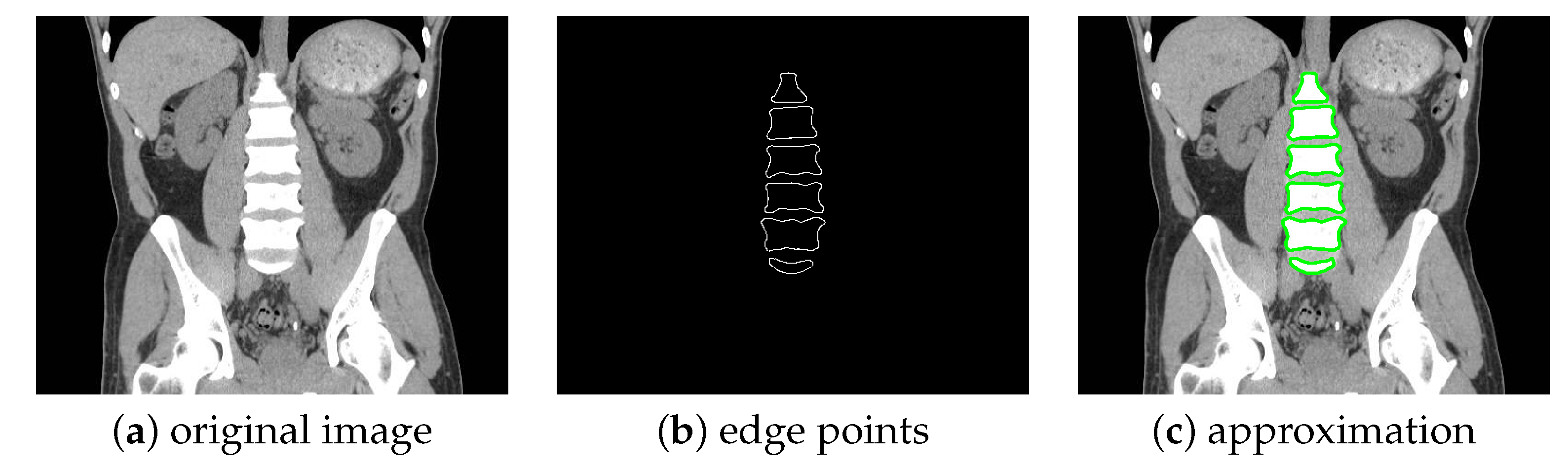
We then consider a coronal slice obtained from the MedPix database (MedPix database, https://medpix.nlm.nih.gov/, accessed on 1 September 2021), see Figure 11. For our testing, we focus our attention on the lumbar spine, whose edge points are shown in Figure 11b and approximated in Figure 11c.
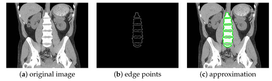
Figure 11.
Recognition and approximation of different profiles from a human lumbar spine. The original image (a) is treated to obtain the edge points (b). The six approximations are given in (c).
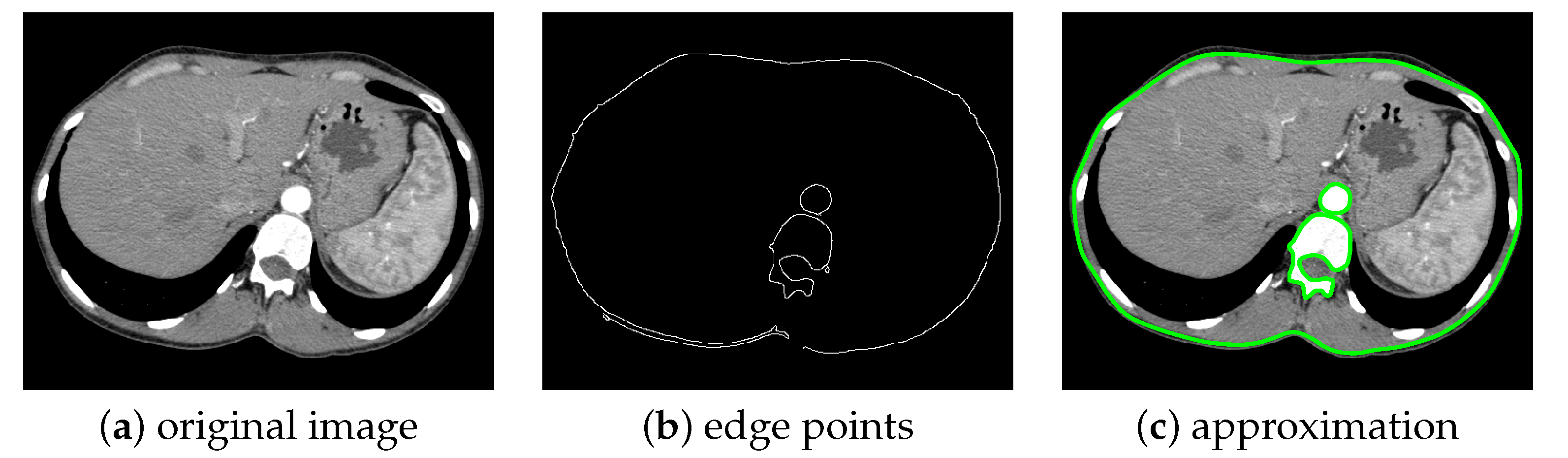
For the last simulation, we consider a axial X-ray CT slice of a human lumbar vertebra, see Figure 12. The image has been obtained by the repository [34]. In Figure 12b we provide the three sets of edge points chosen to be approximated, and corresponding to the external profile of the body section; the vertebra, where it is possible to distinguish body, transverse process and spinous process; the abdominal aorta. In Figure 12c we show the superimposition of three distinct approximations to the original image.

Figure 12.
Recognition and approximation of different profiles in a CT slice. The original X-ray CT axial image (a) is processed and three sets of edge points are selected (b), corresponding to the body profile, the lumbar vertebra and the aorta; the three approximations obtained are then superimposed in (c). Note the presence of outliers in (b).
4.5. Quantitative Evaluation and Discussions
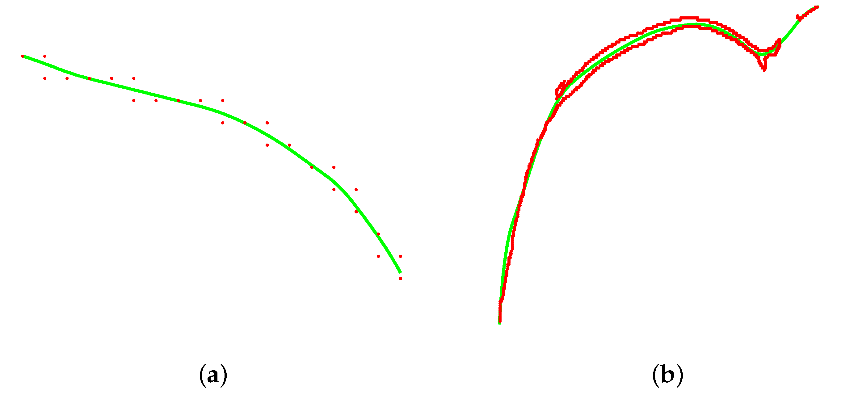
The indicators computed on each profile of each image are provided in Table 1, Table 2 and Table 3. When considering the RMSE, MAE and , all approximations show a quite satisfying performance. In particular, having normalized the directed Hausdorff distance, we can conclude that the error is always below , with the highest values coming from the lumbar spine. Only a few profiles have a Jaccard index lower than ; the lowest possible is that of the body in Figure 12 (61.41% ca.). However, one should consider that this indicator is not reliable when applied to point sets containing a high number of outliers, which is the case for this specific profile, see Figure 13b: the local approximation is able to capture the underlying trend of the data and preserve the monotonicity, but due to the presence of an excessive number of erroneous points, this indicator is not fully representative of the situation. On the contrary, the edge points from Figure 9 are noisy but contain a limited number of outliers; an example of a small local tubular neighborhood and its approximation is given in Figure 13a.

Table 1.
Indicators for the examples in Figure 6 and Figure 7. For each profile, we report: the Root Mean Squared Error (RMSE), the Mean Absolute Error (MAE), the normalized directed Hausdorff distance and the Jaccard index J. Here, fit1, fit2 and fit3 stand, respectively, for quadratic polynomial, piecewise cubic and smoothing spline fitting. For each figure and each indicator, the best performance is reported in bold.
Table 2.
Indicators for the examples in Figure 8 and Figure 9. For each profile we report: the Root Mean Squared Error (RMSE), the Mean Absolute Error (MAE), the normalized directed Hausdorff distance and the Jaccard index J. Here, fit1, fit2 and fit3 stand, respectively, for quadratic polynomial, piecewise cubic and smoothing spline fitting. For each figure and each indicator, the best performance is reported in bold.
Table 3.
Indicators for the examples in Figure 10, Figure 11 and Figure 12. For each profile we report: the Root Mean Squared Error (RMSE), the Mean Absolute Error (MAE), the normalized directed Hausdorff distance and the Jaccard index J. Here, fit1, fit2 and fit3 stand, respectively, for quadratic polynomial, piecewise cubic and smoothing spline fitting. For each figure and each indicator, the best performance is reported in bold.

All in all, it might be concluded that the method can successfully reconstruct planar curvilinear profiles, but its success is inevitably linked to the quality of the segmentation: as observed in the qualitative discussion of Figure 7, the Canny edge detection algorithm was unable to identify the stalk of the mushroom in its entirety.
We compared the generalization capability of wQISAs with that of other fitting methods implemented in MATLAB: quadratic polynomial, piecewise cubic and smoothing spline fitting. When considering RMSE, MAE and , our methods outperforms its competitors; however, in a few cases the results are comparable. In terms of the Jaccard index, the results are more fluid: as previously observed, this is partly justified by the presence of outliers in some point clouds, which makes this indicator not always trustworthy.
To provide a complete analysis of the experimental results, Table 4 provides the number of tubular neighborhoods, the number of edge points and the execution times for all the examples shown in the paper.
5. Conclusions
In this work, we have proposed a novel method to recognize and approximate closed and open 1-manifolds in digital images. Based on the Weighted Quasi-Interpolant Spline Approximation family, our approach can provide a sequence of parametrizations connected continuously, except in correspondence with the identified cusps, where we impose continuity. For each local approximation, the number of knots in the knot vectors and the free parameter k are tuned by cross-validation, to limit under- and overfitting. Being based on the quasi-interpolation paradigm, the method is computationally efficient because it does not involve least-square approximation routines. Experimental results on a set of real digital images show a good performance on real data.
As a future development of the method, we intend to extend it to the case of space curves, that is, to non planar profiles embedded into the Euclidean space, and to curves with non-manifold configurations, such as knots and self-intersections. A typical solution for dealing with complicated image borders is to consider arcs and line segments at the same time [1]; in our case, our method can be iterated on the single 1-manifold arcs by decomposing a general profile into segments.
Author Contributions
Conceptualization, A.R. and S.B.; methodology, A.R.; software, A.R.; validation, A.R.; formal analysis, A.R.; investigation, A.R.; resources, A.R. and S.B.; data curation, A.R.; writing—original draft preparation, A.R.; writing—review and editing, A.R. and S.B.; visualization, A.R.; supervision, S.B.; funding acquisition, S.B. All authors have read and agreed to the published version of the manuscript.
Funding
This research has been made possible by the contribution granted by CNR in the framework of the Scientific Cooperation Agreement CNR-CNRST (Morocco), under the bilateral agreement n. SAC.AD002.014.032, and by the project POR FSE, Programma Operativo Regione Liguria, 2014–2020 grant number RLOF18ASSRIC/68/1.
Institutional Review Board Statement
Not Applicable.
Informed Consent Statement
Not Applicable.
Data Availability Statement
Data available online in publicly accessible repositories, see Section 4.
Acknowledgments
The authors thank Bianca Falcidieno and Michela Spagnuolo for the fruitful discussions.
Conflicts of Interest
The authors declare no conflict of interest. The funders had no role in the design of the study; in the collection, analyses, or interpretation of data; in the writing of the manuscript, or in the decision to publish the results.
References
- Nguyen, T.P.; Debled-Rennesson, I. Decomposition of a Curve into Arcs and Line Segments Based on Dominant Point Detection. In Image Analysis; Heyden, A., Kahl, F., Eds.; Springer: Berlin/Heidelberg, Germany, 2011; pp. 794–805. [Google Scholar]
- Cheney, E.W. Approximation Theory, Wavelets and Applications; NATO Science Series; Springer Science & Business Media: Berlin/Heidelberg, Germany, 1995; Volume 454, pp. 37–45. [Google Scholar]
- Sablonnière, P. Univariate spline quasi-interpolants and applications to numerical analysis. In Rendiconti del Seminario Matematico; Università Degli Studi di Torino/Politecnico di Torino: Turin, Italy, 2005; Volume 63, pp. 211–222. [Google Scholar]
- Bernstein, S.N. Démonstration du théorème de Weierstrass fondée sur le calcul des probabilités. Commun. Société Mathématique Kharkow 1912, 13, 1–2. [Google Scholar]
- Marsden, M.; Schoenberg, I.J. On Variation Diminishing Spline Approximation Methods; de Boor, C., Ed.; Springer Science & Business Media: Berlin/Heidelberg, Germany, 1988; Volume 2, pp. 247–268. [Google Scholar] [CrossRef]
- Lyche, T.; Mørken, K. Spline Methods Draft; University of Oslo: Oslo, Norway, 2011. [Google Scholar]
- Barrera, D.; Ibáñez, M.J.; Sablonnière, P.; Sbibih, D. Near-Best Univariate Spline Discrete Quasi-Interpolants on Nonuniform Partitions. Constr. Approx. 2008, 28, 237–251. [Google Scholar] [CrossRef] [Green Version]
- Remogna, S.; Sablonnière, P. On trivariate blending sums of univariate and bivariate quadratic spline quasi-interpolants on bounded domains. Comput. Aided Geom. Des. 2011, 28, 89–101. [Google Scholar] [CrossRef] [Green Version]
- Ibáñez, M.J.; Barrera, D.; Maldonado, D.; Yáñez, R.; Roldán, J.B. Non-Uniform Spline Quasi-Interpolation to Extract the Series Resistance in Resistive Switching Memristors for Compact Modeling Purposes. Mathematics 2021, 9, 2159. [Google Scholar] [CrossRef]
- Remogna, S. Bivariate C2 cubic spline quasi-interpolants on uniform Powell–Sabin triangulations of a rectangular domain. Adv. Comput. Math. 2012, 36, 39–65. [Google Scholar] [CrossRef]
- Sbibih, D.; Serghini, A.; Tijini, A.; Zidna, A. Superconvergent C1 cubic spline quasi-interpolants on Powell-Sabin partitions. BIT Numer. Math. 2015, 55, 797–821. [Google Scholar] [CrossRef]
- Sbibih, D.; Serghini, A.; Tijini, A. Superconvergent quadratic spline quasi-interpolants on Powell–Sabin partitions. Appl. Numer. Math. 2015, 87, 74–86. [Google Scholar] [CrossRef]
- Eddargani, S.; Ibáñez, M.J.; Lamnii, A.; Lamnii, M.; Barrera, D. Quasi-Interpolation in a Space of C2 Sextic Splines over Powell–Sabin Triangulations. Mathematics 2021, 9, 2276. [Google Scholar] [CrossRef]
- Sbibih, D.; Serghini, A.; Tijini, A. Superconvergent local quasi-interpolants based on special multivariate quadratic spline space over a refined quadrangulation. Appl. Math. Comput. 2015, 250, 145–156. [Google Scholar] [CrossRef]
- Barrera, D.; Ibáñez, M.; Remogna, S. On the Construction of Trivariate Near-Best Quasi-Interpolants Based on C2 Quartic Splines on Type-6 Tetrahedral Partitions. J. Comput. Appl. Math. 2017, 311, 252–261. [Google Scholar] [CrossRef]
- Raffo, A.; Biasotti, S. Weighted quasi-interpolant spline approximations: Properties and applications. Numer. Algorithms 2021, 87, 819–847. [Google Scholar] [CrossRef]
- Raffo, A.; Biasotti, S. Data-driven quasi-interpolant spline surfaces for point cloud approximation. Comput. Graph. 2020, 89, 144–155. [Google Scholar] [CrossRef]
- Barsky, B.A.; DeRose, A.D. Geometric Continuity of Parametric Curves; Technical Report UCB/CSD-84-205; EECS Department, University of California: Berkeley, CA, USA, 1984. [Google Scholar]
- DeRose, T.D.; Barsky, B.A. An Intuitive Approach to Geometric Continuity for Parametric Curves and Surfaces. In Computer-Generated Images; Magnenat-Thalmann, N., Thalmann, D., Eds.; Springer: Tokyo, Japan, 1985; pp. 159–175. [Google Scholar]
- Said Mad Zain, S.A.A.A.; Misro, M.Y.; Miura, K.T. Generalized Fractional Bézier Curve with Shape Parameters. Mathematics 2021, 9, 2141. [Google Scholar] [CrossRef]
- Farin, G. Curves and Surfaces for CAGD: A Practical Guide, 5th ed.; Morgan Kaufmann Publishers Inc.: San Francisco, CA, USA, 2001. [Google Scholar]
- Mizutani, K.; Kawaguchi, K. Curve approximation by G1 arc splines with a limited number of types of curvature and length. Comput. Aided Geom. Des. 2021, 90, 102036. [Google Scholar] [CrossRef]
- Canny, J. A Computational Approach to Edge Detection. IEEE Trans. Pattern Anal. Mach. Intell. 1986, PAMI-8, 679–698. [Google Scholar] [CrossRef]
- Heath, M.; Sarkar, S.; Sanocki, T.; Bowyer, K. Comparison of Edge Detectors: A Methodology and Initial Study. Comput. Vis. Image Underst. 1998, 69, 38–54. [Google Scholar] [CrossRef]
- Williams, I.; Bowring, N.; Svoboda, D. A performance evaluation of statistical tests for edge detection in textured images. Comput. Vis. Image Underst. 2014, 122, 115–130. [Google Scholar] [CrossRef]
- Conti, C.; Romani, L.; Schenone, D. Semi-automatic spline fitting of planar curvilinear profiles in digital images using the Hough transform. Pattern Recognit. 2018, 74, 64–76. [Google Scholar] [CrossRef]
- Abate, M.; Francesca, T. Curves and Surfaces; Springer: Mailand, Italy, 2012. [Google Scholar] [CrossRef]
- Arlot, S.; Celisse, A. A survey of cross-validation procedures for model selection. Stat. Surv. 2010, 4, 40–79. [Google Scholar] [CrossRef]
- Hastie, T.; Tibshirani, R.; Friedman, J. The Elements of Statistical Learning; Springer Series in Statistics; Springer: New York, NY, USA, 2001. [Google Scholar]
- Giraudot, S.; Cohen-Steiner, D.; Alliez, P. Noise-Adaptive Shape Reconstruction from Raw Point Sets. Comput. Graph. Forum 2013, 32, 229–238. [Google Scholar] [CrossRef] [Green Version]
- Taha, A.A.; Hanbury, A. Metrics for evaluating 3D medical image segmentation: Analysis, selection, and tool. BMC Med. Imaging 2015, 15, 29. [Google Scholar] [CrossRef] [PubMed] [Green Version]
- Martin, D.; Fowlkes, C.; Tal, D.; Malik, J. A Database of Human Segmented Natural Images and its Application to Evaluating Segmentation Algorithms and Measuring Ecological Statistics. In Proceedings of the Proceedings Eighth IEEE International Conference on Computer Vision—ICCV 2001, Vancouver, BC, Canada, 7–14 July 2001; Volume 2, pp. 416–423. [Google Scholar]
- Hu, Y.; Schneider, T.; Gao, X.; Zhou, Q.; Jacobson, A.; Zorin, D.; Panozzo, D. TriWild: Robust Triangulation with Curve Constraints. ACM Trans. Graph. 2019, 38, 52:1–52:15. [Google Scholar] [CrossRef]
- Hazarika, H.J.; Handique, A.; Ravikumar, S. DICOM-based medical image repository using DSpace. Collect. Curation 2020, 39, 105–115. [Google Scholar] [CrossRef]


Publisher’s Note: MDPI stays neutral with regard to jurisdictional claims in published maps and institutional affiliations. |
© 2021 by the authors. Licensee MDPI, Basel, Switzerland. This article is an open access article distributed under the terms and conditions of the Creative Commons Attribution (CC BY) license (https://creativecommons.org/licenses/by/4.0/).