Fractional Dynamics of Vector-Borne Infection with Sexual Transmission Rate and Vaccination

Abstract

New fractional operators have the aim of attracting nonlocal problems that display fractal behaviour; and thus fractional derivatives have applications in long-term relation description along with micro-scaled and macro-scaled phenomena. Formulated by fractional operators, the formulation of a dynamical system is used in applications for the description of systems with long-range interactions. Vector-borne illnesses are one of the world’s most serious public health issues with a large economic impact on the nations that are impacted. Population increase, urbanization, globalization, and a lack of public health infrastructure have all had a role in the introduction and reemergence of vector-borne illnesses during the last four decades. The control of these infections are important to lessen the economic burden of vector-borne diseases in infected regions. In this research work, we formulate the transmission process of Zika virus with the impact of sexual incidence rate and vaccination in terms of mathematics. We presented the fundamental theory of fractional operators Caputo–Fabrizio (CF) and Atangana–Baleanu (AB) for the analysis of the proposed system. We examine our system of Zika infection and determined the endemic indicator through a next-generation matrix technique. The uniqueness and existence of the solution has been investigated through fixed point theory. Accordingly, a numerical method has been introduced to investigate the dynamical nature of the system and make a comparison of the outcomes of the operators. The impact of different input factors has been conceptualized through dynamical behaviour of the system. We observed that lowering the index of memory, the fractional system provides accurate results about the recommended Zika dynamics and dramatically reduces infected people. It has been proved that high efficacy of a vaccine can lower the level of infection. Moreover, the impact of other parameters on the system of Zika virus infection are highlighted through numerical results.

1. Introduction

Vector-borne illnesses are transferred through hematophagous arthropods such as triatomine bugs, sand flies, ticks and mosquitoes; these infections are found all over the world. Viruses cause the most common vector-borne illnesses all around the world, among these are viral infection dengue, malaria, west Nile virus infection and Zika virus infection. In this paper, we will mainly focus on the transmission phenomena of the Zika virus illness. This viral infection was found in monkeys and the first case in humans was reported in Tanzania and Uganda in 1952. In 1960 and 1980, a few cases were found in Africa and Asia and then the virus of Zika expanded to other parts of the world. This dangerous infection is then spread to many countries in the world with a highest incidence. The symptoms of this condition include headache, rash, fever, muscle pain, conjunctivitis, discomfort of joints and malaise. Zika is a mosquito-borne virus transmitted mostly by Aedes mosquitoes. Aside from that, Zika virus can be passed from mother to child during delivery or shortly after birth. Sexual interactions and blood transfusions are also responsible for the spread of Zika virus.

Mathematical models are a significant tool for understanding different natural phenomena [1,2,3]. Several mathematical models [4,5,6,7,8,9,10] have been reported in the last several years to analyze the transmission process of the Zika virus. The researchers in their work included the below main factors in models: (i) sexual transmission and vector [4,11]; (ii) vector and sexual transmission; (iii) vertical and vector transmission [5,12]; and (iv) optimum control of pesticide spraying, other preventives, and treatment [6,11]. Fractional calculus is a leading framework for the inspection of the impact of the index of memory on dynamics of infections for producing more realistic results. Many academics have investigated how fractional extensions of integer-order mathematical models describe natural facts in a systematic fashion [13,14,15,16]. Further, applications of the fractional differential system have been studied in [17,18]. Fractional-order derivatives have grown in popularity in recent years, and they are now frequently employed in modeling real-world events and exploring disease transmission and control [19,20,21,22,23]. In recent years, various investigations with biological models using fractional-order derivatives have been carried out [24,25,26,27].

As a result of the foregoing study, we have chosen to offer a model for the transmission process of Zika virus infection with the help of fractional operators. The other sections of this research are structured as: Section 2 contains the essential definitions and assertions of the fractional theory of CF and AB operators. In Section 3, we build a Zika virus infection model with the influence of sexual transmission in the structure of fractional order CF and AB derivatives as well as to analyze the steady-states and endemic indicators of the proposed system. We used the theory of fixed point to prove the uniqueness and existence of the suggested system’s solution in Section 4. We inspect the model in the framework of the Atangana–Baleanu derivative in Section 5 of the paper. In Section 6, we visualize the dynamical nature of the system with the impact of different input factors and perform a comparative analysis of the operators. Finally, the overall work is summarized in Section 7 of the paper.

2. Fractional Theory

The fundamental results and definitions of the fractional Caputo–Fabrizio (CF) and Atangana–Baleanu (AB) operators are provided in this section of the paper. These operators as fractional derivatives use the generalized Mittag–Leffler function as the non-local and non-singular kernel and accepts all properties of fractional derivatives. Then, we investigate our model with the help of these results and definitions. First, we present the idea of a CF operator as given below:

Definition 1.

Take a function $h\in H^1(a,b)$, then the CF fractional derivative [28] is as follows:

$$\begin{array}{c}\hfill D_t^{\wp }\left(g\left(t\right)\right)=\frac{\mathcal{U}(\wp )}{1-\wp }{\int }_a^t{g}^{\prime }\left(x\right)exp\left[-\wp \frac{t-x}{1-\wp }\right]dx,\end{array}$$

(1)

where b is greater than a and $\mathcal{U}\left(\tau \right)$ indicates the normality [28] with the condition that $\wp \in [0,1]$. In the case, if $h\notin H^1(a,b)$, we have:

$$\begin{array}{c}\hfill D_t^{\wp }\left(g\left(t\right)\right)=\frac{\wp U(\wp )}{1-\wp }{\int }_a^t(g\left(t\right)-g\left(x\right))exp\left[-\wp \frac{t-x}{1-\wp }\right]dx.\end{array}$$

(2)

Remark 1.

In the case where $\alpha =\frac{1-\wp }{\wp }\in [0,\infty )$ and $\wp =\frac{1}{1+\alpha }\in [0,1]$, then Equation (2) implies the below:

$$\begin{array}{c}\hfill D_t^{\wp }\left(g\left(t\right)\right)=\frac{M\left(\alpha \right)}{\alpha }{\int }_a^t{g}^{\prime }\left(x\right)e^{[-\frac{t-x}{\alpha }]}dx,M\left(0\right)=M(\infty )=1.\end{array}$$

(3)

We also have:

$$\begin{array}{c}\hfill \underset{\alpha ⟶0}{lim}\frac{1}{\alpha }exp\left[-\frac{t-x}{\alpha }\right]=\delta (x-t).\end{array}$$

(4)

Definition 2

([29]). For a given function g, the integral in the fractional framework is given as below:

$$\begin{array}{c}\hfill I_t^{\wp }\left(g\left(t\right)\right)=\frac{2(1-\wp )}{(2-\wp )U(\wp )}g\left(t\right)+\frac{2\wp }{(2-\wp )U(\wp )}{\int }_0^{t}g\left(u\right)du,t\ge 0,\end{array}$$

(5)

in which the term ℘ indicates the fractional order of the integral with the condition $0<\wp <1$.

Remark 2.

The above Definition 2 gives the following:

$$\begin{array}{c}\hfill \frac{2(1-\wp )}{(2-\wp )\mathcal{U}(\wp )}+\frac{2\wp }{(2-\wp )\mathcal{U}(\wp )}=1,\end{array}$$

(6)

which implies that $\mathcal{U}(\wp )=\frac{2}{2-\wp }$, $0<\wp <1$. The researchers in [29], introduced the following with the help of (6)

$$\begin{array}{c}\hfill D_t^{\wp }\left(g\left(t\right)\right)=\frac{1}{1-\wp }{\int }_0^t{g}^{\prime }\left(x\right)exp\left[\wp \frac{t-x}{1-\wp }\right]dx,\end{array}$$

(7)

in which the term ℘ is the fractional order with $0<\wp <1$.

In the upcoming part, we present the concept of the AB fractional operator [30]. We will use these ideas in the analysis of Zika dynamics.

Definition 3.

Consider h in a way that $h\in H^1(a,b)$, then the AB derivative in Caputo form is indicated by ABC and is given by:

$${}_a^{ABC}{D}_t^{\wp }h\left(t\right)=\frac{U(\wp )}{1-\wp }{\int }_a^t{h}^{\prime }\left(\xi \right)E_{\wp }\left[-\wp \frac{{(t-\xi )}^{\wp }}{1-\wp }\right]d\xi ,$$

where the fractional order $\ell \in [0,1]$ and b is greater than a.

Definition 4.

For the ABC derivative, the fractional integral is indicated by ${}_a^{ABC}{I}_t^{\wp }h\left(t\right)$ and is given by:

$${}_a^{ABC}{I}_t^{\wp }h\left(t\right)=\frac{1-\wp }{U(\wp )}f\left(t\right)+\frac{\wp }{U(\wp )\mathsf{\Gamma }(\wp )}{\int }_a^{t}h\left(\xi \right){(t-\xi )}^{\wp -1}d\xi .$$

Theorem 1

([30]). Take h in a way that $h\in C[a,b]$, then the below is fulfilled:

$$\parallel {}_a^{ABC}{D}_t^{\wp }\left(h\left(t\right)\right)\parallel <\frac{U(\wp )}{1-\wp }\parallel h\left(t\right)\parallel ,where\parallel h\left(t\right)\parallel =ma{x}_{a\le t\le b}\left|h\left(t\right)\right|.$$

In the above ABC derivative, the Lipschitz condition is satisfied in the following manner [30]:

$$\parallel {}_a^{ABC}{D}_t^{\wp }{h}_1\left(t\right)-{}_a^{ABC}{D}_t^{\wp }{h}_2\left(t\right)\parallel <{\nearrow }_1\parallel h_1\left(t\right)-h_2\left(t\right)\parallel .$$

Theorem 2

([30]). Let us take the following fractional system:

$${}_a^{ABC}{D}_t^{\wp }h\left(t\right)=w\left(t\right),$$

then there is a unique solution of the above system given by:

$$h\left(t\right)=\frac{1-\wp }{U(\wp )}w\left(t\right)+\frac{\wp }{U(\wp )\mathsf{\Gamma }(\wp )}{\int }_a^{t}w\left(\xi \right){(t-\xi )}^{\wp -1}d\xi .$$

3. Evaluation of the Fractional Dynamics

The transmission phenomena of Zika virus infection with the effect of sexual transmission rate and vaccination in terms of mathematics has been introduced through this study. We categorized the total hosts’ size $N_h$ into four classes, which are, susceptible $S_h$, exposed $E_h$, infected $I_h$, recovered $R_h$ compartments while the mosquitoes’ size $N_v$ is categorized into three classes, which are susceptible $S_v$, exposed $E_v$ and infected $I_v$ classes. In our formulation, we assumed the recruitment rate ${\mathsf{\Pi }}_h$ and ${\mathsf{\Pi }}_v$ for humans and vectors, respectively, while the rate of natural death of humans and vectors is taken to be ${\mu }_h$ and ${\mu }_v$. The vaccination rate of susceptible humans is considered to be p, while the recovery rate of the infected class is denoted by $\gamma$. The force of infection of humans and vectors is taken to be $\frac{{\beta }_{1}b{I}_v}{N_h}$ and $\frac{{\beta }_{2}b{I}_h}{N_h}$ while the transmission through sexual interaction of humans is considered. Then, the system of Zika virus infection with the above assumptions is:

$$\left\{\begin{array}{ccc}\hfill \frac{d{S}_h}{dt}& =& {\mathsf{\Pi }}_h-\frac{{\beta }_{1}b{I}_v}{N_h}{S}_h-\frac{{\beta }_{2}c{I}_h}{N_h}{S}_h-p{S}_h-{\mu }_h{S}_h,\hfill \\ \hfill \frac{d{E}_h}{dt}& =& \frac{{\beta }_{1}b{I}_v}{N_h}{S}_h+\frac{{\beta }_{2}c{I}_h}{N_h}{S}_h-({\rho }_1+{\mu }_h)E_h,\hfill \\ \hfill \frac{d{I}_h}{dt}& =& {\rho }_1{E}_h-(\gamma +{\mu }_h)I_h,\hfill \\ \hfill \frac{d{R}_h}{dt}& =& p{S}_h+\gamma I_h-{\mu }_h{R}_h,\hfill \\ \hfill \frac{d{S}_v}{dt}& =& {\mathsf{\Pi }}_v-\frac{{\beta }_{3}b{I}_h}{N_h}{S}_v-(d+{\mu }_v)S_v,\hfill \\ \hfill \frac{d{E}_v}{dt}& =& \frac{{\beta }_{3}b{I}_h}{N_h}{S}_v-(d+{\mu }_v+{\rho }_2)E_v,\hfill \\ \hfill \frac{d{I}_v}{dt}& =& {\rho }_2{E}_v-(d+{\mu }_v)I_v,\hfill \end{array}\right.$$

(8)

with

$$S_h\left(0\right)=S_{h0},E_h\left(0\right)=E_{h0},I_h\left(0\right)=I_{h0},R_h\left(0\right)=R_{h0},$$

$$S_v\left(0\right)=S_{v0},E_v\left(0\right)=E_{v0}and{I}_v\left(0\right)=I_{v0}.$$

In the above formulation, the input factor d indicates the effective rate of mosquito control. There are numerous applications of fractional calculus in science, including mathematical biology. It has been demonstrated that fractional frameworks can more precisely depict the dynamics of infections than traditional integer order derivatives. The above model of Zika virus infection can be written through the CF operator as:

$$\left\{\begin{array}{ccc}\hfill {}_0^{CF}{D}_t^{\wp }{S}_h& =& {\mathsf{\Pi }}_h-\frac{{\beta }_{1}b{I}_v}{N_h}{S}_h-\frac{{\beta }_{2}c{I}_h}{N_h}{S}_h-p{S}_h-{\mu }_h{S}_h,\hfill \\ \hfill {}_0^{CF}{D}_t^{\wp }{E}_h& =& \frac{{\beta }_{1}b{I}_v}{N_h}{S}_h+\frac{{\beta }_{2}c{I}_h}{N_h}{S}_h-({\rho }_1+{\mu }_h)E_h,\hfill \\ \hfill {}_0^{CF}{D}_t^{\wp }{I}_h& =& {\rho }_1{E}_h-(\gamma +{\mu }_h)I_h,\hfill \\ \hfill {}_0^{CF}{D}_t^{\wp }{R}_h& =& p{S}_h+\gamma I_h-{\mu }_h{R}_h,\hfill \\ \hfill {}_0^{CF}{D}_t^{\wp }{S}_v& =& {\mathsf{\Pi }}_v-\frac{{\beta }_{3}b{I}_h}{N_h}{S}_v-(d+{\mu }_v)S_v,\hfill \\ \hfill {}_0^{CF}{D}_t^{\wp }{E}_v& =& \frac{{\beta }_{3}b{I}_h}{N_h}{S}_v-(d+{\mu }_v+{\rho }_2)E_v,\hfill \\ \hfill {}_0^{CF}{D}_t^{\wp }{I}_v& =& {\rho }_2{E}_v-(d+{\mu }_v)I_v,\hfill \end{array}\right.$$

(9)

where ℘ is the order of CF fractional operator. The positive invariant region of the hypothesized fractional system of Zika virus infection is given below:

Theorem 3.

Let us assume the set Ω in a manner that $\mathsf{\Omega }=\{(S_h,E_h,I_h,R_h,S_v,E_v,I_v)\in R_{+}^7:0\le S_h+E_h+I_h+R_h\le M_1,0\le S_v+E_v+I_v\le M_2\}$ is a positive invariant for our model (9) of Zika virus disease.

Model Analysis

The suggested model (9) of Zika virus infection for a steady-state and stability is investigated in this portion of the study. First, we investigate the suggested system’s disease-free equilibrium, which is denoted by $E_0$ and is given by:

$$E_0=\left(\frac{{\mathsf{\Pi }}_h}{(p+{\mu }_h)},0,0,\frac{p{\mathsf{\Pi }}_h}{{\mu }_h(p+{\mu }_h)},\frac{{\mathsf{\Pi }}_v}{(d+{\mu }_v)},0,0\right).$$

For the reproduction number [31,32,33], we utilize the method of next-generation matrix in the following manner:

$$F=\left[\begin{array}{cccc}0& A_1{S}_h^0& 0& A_2{S}_h^0\\ 0& 0& 0& 0\\ 0& A_3{S}_h^0& 0& 0\\ 0& 0& 0& 0\end{array}\right],$$

$$V=\left[\begin{array}{cccc}k1& 0& 0& 0\\ -{\rho }_1& k2& 0& 0\\ 0& 0& k3& 0\\ 0& 0& -{\rho }_2& k4\end{array}\right],$$

where we have $A_1=\frac{{\beta }_{2}c}{N_h},A_2=\frac{{\beta }_{1}b}{N_h},A_3=\frac{{\beta }_{3}b}{N_h},k1={\rho }_1+{\mu }_h,k2=\gamma +{\mu }_h,k3={\rho }_v+{\mu }_v+d$ and $k4={\mu }_v+d.$ Further, we have the following, after simplifications:

$$\rho \left(F{V}^{-1}\right)=\frac{1}{2k1k2k3k4}\left(A_1{S}_h^0{\rho }_{1}k3k4+{\{{\left(A_1{S}_h^0{\rho }_{1}k3k4\right)}^2+4A_2{A}_3{S}_h^0{S}_v^0{\rho }_1{\rho }_{2}k1k2k3k4\}}^{\frac{1}{2}}\right),$$

which implies that

$${\mathcal{R}}_0=\frac{1}{2k1k2k3k4}\left(A_1{S}_h^0{\rho }_{1}k3k4+{\{{\left(A_1{S}_h^0{\rho }_{1}k3k4\right)}^2+4A_2{A}_3{S}_h^0{S}_v^0{\rho }_1{\rho }_{2}k1k2k3k4\}}^{\frac{1}{2}}\right).$$

This is the required ${\mathcal{R}}_0$ of our system of Zika infection, which illustrates the status of infection in the community.

Theorem 4.

The infection-free steady-state of the Zika virus infection system (9) is locally asymptotically stable for ${\mathcal{R}}_0<1$ and is unstable in another status.

4. Solution Analysis via CF

In this part, we have focused on the analysis of the solutions of the hypothesized fractional system of Zika virus infection. Fixed point theory will be applied to investigate the existence of solution (9). The following steps are followed for this purpose:

$$\left\{\begin{array}{ccc}\hfill S_h\left(t\right)-S_h\left(0\right)& =& {}_0^{CF}{I}_t^{\wp }\left\{{\mathsf{\Pi }}_h-\frac{{\beta }_{1}b{I}_v}{N_h}{S}_h-\frac{{\beta }_{2}c{I}_h}{N_h}{S}_h-p{S}_h-{\mu }_h{S}_h\right\},\hfill \\ \hfill E_h\left(t\right)-E_h\left(0\right)& =& {}_0^{CF}{I}_t^{\wp }\left\{\frac{{\beta }_{1}b{I}_v}{N_h}{S}_h+\frac{{\beta }_{2}c{I}_h}{N_h}{S}_h-({\rho }_1+{\mu }_h)E_h\right\},\hfill \\ \hfill I_h\left(t\right)-I_h\left(0\right)& =& {}_0^{CF}{I}_t^{\wp }\left\{{\rho }_1{E}_h-(\gamma +{\mu }_h)I_h\right\},\hfill \\ \hfill R_h\left(t\right)-R_h\left(0\right)& =& {}_0^{CF}{I}_t^{\wp }\left\{p{S}_h+\gamma I_h-{\mu }_h{R}_h\right\},\hfill \\ \hfill S_v\left(t\right)-S_v\left(0\right)& =& {}_0^{CF}{I}_t^{\wp }\left\{{\mathsf{\Pi }}_v-\frac{{\beta }_{3}b{I}_h}{N_h}{S}_v-(d+{\mu }_v)S_v\right\},\hfill \\ \hfill E_v\left(t\right)-E_v\left(0\right)& =& {}_0^{CF}{I}_t^{\wp }\left\{\frac{{\beta }_{3}b{I}_h}{N_h}{S}_v-(d+{\mu }_v+{\rho }_2)E_v\right\},\hfill \\ \hfill I_v\left(t\right)-E_v\left(0\right)& =& {}_0^{CF}{I}_t^{\wp }\left\{{\rho }_2{E}_v-(d+{\mu }_v)I_v\right\}.\hfill \end{array}\right.$$

(10)

We used the concepts of the research [29] and obtained the below:

$$\begin{array}{ccc}\hfill S_h\left(t\right)-S_h\left(0\right)& =& \frac{2(1-\wp )}{(2-\wp )U(\wp )}\left\{{\mathsf{\Pi }}_h-\frac{{\beta }_{1}b{I}_v}{N_h}{S}_h-\frac{{\beta }_{2}c{I}_h}{N_h}{S}_h-p{S}_h-{\mu }_h{S}_h\right\}\hfill \\ \\ & & +\frac{2\wp }{(2-\wp )U(\wp )}{\int }_0^t\left\{{\mathsf{\Pi }}_h-\frac{{\beta }_{1}b{I}_v}{N_h}{S}_h-\frac{{\beta }_{2}c{I}_h}{N_h}{S}_h-p{S}_h-{\mu }_h{S}_h\right\}dy,\hfill \\ \\ \hfill E_h\left(t\right)-E_h\left(0\right)& =& \frac{2(1-\wp )}{(2-\wp )U(\wp )}\left\{\frac{{\beta }_{1}b{I}_v}{N_h}{S}_h+\frac{{\beta }_{2}c{I}_h}{N_h}{S}_h-({\rho }_1+{\mu }_h)E_h\right\}\hfill \\ \\ & & +\frac{2\wp }{(2-\wp )U(\wp )}{\int }_0^t\left\{\frac{{\beta }_{1}b{I}_v}{N_h}{S}_h+\frac{{\beta }_{2}c{I}_h}{N_h}{S}_h-({\rho }_1+{\mu }_h)E_h\right\}dy,\hfill \\ \\ \hfill I_h\left(t\right)-I_h\left(0\right)& =& \frac{2(1-\wp )}{(2-\wp )U(\wp )}\left\{{\rho }_1{E}_h-(\gamma +{\mu }_h)I_h\right\}\hfill \\ \\ & & +\frac{2\wp }{(2-\wp )U(\wp )}{\int }_0^t\left\{{\rho }_1{E}_h-(\gamma +{\mu }_h)I_h\right\}dy,\hfill \\ \\ \hfill R_h\left(t\right)-R_h\left(0\right)& =& \frac{2(1-\wp )}{(2-\wp )U(\wp )}\left\{p{S}_h+\gamma I_h-{\mu }_h{R}_h\right\}\hfill \\ \\ & & +\frac{2\wp }{(2-\wp )U(\wp )}{\int }_0^t\left\{p{S}_h+\gamma I_h-{\mu }_h{R}_h\right\}dy,\hfill \\ \\ \hfill S_v-S_v\left(0\right)& =& \frac{2(1-\wp )}{(2-\wp )U(\wp )}\left\{\frac{{\beta }_{3}b{I}_h}{N_h}{S}_v-(d+{\mu }_v+{\rho }_2)E_v\right\}\hfill \\ \\ & & +\frac{2\wp }{(2-\wp )U(\wp )}{\int }_0^t\left\{\frac{{\beta }_{3}b{I}_h}{N_h}{S}_v-(d+{\mu }_v+{\rho }_2)E_v\right\}dy,\hfill \\ \\ \hfill E_v\left(t\right)-E_v\left(0\right)& =& \frac{2(1-\wp )}{(2-\wp )U(\wp )}\left\{\frac{{\beta }_{3}b{I}_h}{N_h}{S}_v-(d+{\mu }_v+{\rho }_2)E_v\right\}\hfill \\ \\ & & +\frac{2\wp }{(2-\wp )U(\wp )}{\int }_0^t\left\{\frac{{\beta }_{3}b{I}_h}{N_h}{S}_v-(d+{\mu }_v+{\rho }_2)E_v\right\}dy,\hfill \\ \\ \hfill I_v-I_v\left(0\right)& =& \frac{2(1-\wp )}{(2-\wp )U(\wp )}\left\{{\rho }_2{E}_v-(d+{\mu }_v)I_v\right\}\hfill \\ \\ & & +\frac{2\wp }{(2-\wp )U(\wp )}{\int }_0^t\left\{{\rho }_2{E}_v-(d+{\mu }_v)I_v\right\}dy.\hfill \end{array}$$

(11)

Further, we have:

$$\left\{\begin{array}{ccc}\hfill L_1(t,S_h)& =& {\mathsf{\Pi }}_h-\frac{{\beta }_{1}b{I}_v}{N_h}{S}_h-\frac{{\beta }_{2}c{I}_h}{N_h}{S}_h-p{S}_h-{\mu }_h{S}_h,\hfill \\ \hfill L_2(t,E_h)& =& \frac{{\beta }_{1}b{I}_v}{N_h}{S}_h+\frac{{\beta }_{2}c{I}_h}{N_h}{S}_h-({\rho }_1+{\mu }_h)E_h,\hfill \\ \hfill L_3(t,I_h)& =& {\rho }_1{E}_h-(\gamma +{\mu }_h)I_h,\hfill \\ \hfill L_4(t,R_h)& =& p{S}_h+\gamma I_h-{\mu }_h{R}_h,\hfill \\ \hfill L_5(t,S_v)& =& {\mathsf{\Pi }}_v-\frac{{\beta }_{3}b{I}_h}{N_h}{S}_v-(d+{\mu }_v)S_v,\hfill \\ \hfill L_6(t,E_v)& =& \frac{{\beta }_{3}b{I}_h}{N_h}{S}_v-(d+{\mu }_v+{\rho }_2)E_v,\hfill \\ \hfill L_7(t,I_v)& =& {\rho }_2{E}_v-(d+{\mu }_v)I_v.\hfill \end{array}\right.$$

(12)

Theorem 5.

The kernels $L_1,L_2,L_3,L_4,L_5,L_6$ and $L_7$ fulfil the condition of Lipschitz and contraction if the below satisfies:

$$0\le (M+d+\nu )<1.$$

Proof. 

For the above demanded outcomes, we take $S_h$ and $S_{h1}$, and start from $L_1$ in the following manner:

$$\begin{array}{ccc}\hfill L_1(t,S_h)-L_1(t,S_{h1})& =& -\frac{{\beta }_{1}b{I}_v}{N_h}\{S_h\left(t\right)-S_h\left(t_1\right)\}-\frac{{\beta }_{2}c{I}_h}{N_h}\{S_h\left(t\right)-S_h\left(t_1\right)\}-p\{S_h\left(t\right)-S_h\left(t_1\right)\}\hfill \\ \\ & & -{\mu }_h\{S_h\left(t\right)-S_h\left(t_1\right)\}.\hfill \end{array}$$

(13)

After simplification of (13), we attain the below:

$$\begin{array}{ccc}\hfill \parallel L_1(t,S_h)-L_1(t,S_{h1})\parallel & \le & \parallel \frac{{\beta }_{1}b{I}_v}{N_h}\{S_h\left(t\right)-S_h\left(t_1\right)\}\left|\right|+\parallel \frac{{\beta }_{2}c{I}_h}{N_h}\{S_h\left(t\right)-S_h\left(t_1\right)\}\left|\right|\hfill \\ \\ & & +p\parallel \{S_h\left(t\right)-S_h\left(t_1\right)\}\parallel +{\mu }_h\parallel \{S_h\left(t\right)-S_h\left(t_1\right)\}\parallel \hfill \\ \\ \hfill & \le & \parallel \frac{{\beta }_{1}bM}{K}\parallel \parallel S_h\left(t\right)-S_h\left(t_1\right)\left|\right|+\parallel \frac{{\beta }_{2}cM}{K}\parallel \parallel S_h\left(t\right)-S_h\left(t_1\right)\parallel \hfill \\ \\ & & +p\parallel S_h\left(t\right)-S_h\left(t_1\right)\parallel +{\mu }_h\parallel S_h\left(t\right)-S_h\left(t_1\right)\parallel \hfill \\ \\ \hfill & \le & \frac{{\beta }_{1}bM}{K}\parallel S_h\left(t\right)-S_h\left(t_1\right)\left|\right|+\frac{{\beta }_{2}cM}{K}\parallel S_h\left(t\right)-S_h\left(t_1\right)\parallel \hfill \\ \\ & & +p\parallel S_h\left(t\right)-S_h\left(t_1\right)\parallel +{\mu }_h\parallel S_h\left(t\right)-S_h\left(t_1\right)\parallel \hfill \\ \\ \hfill & \le & (\frac{{\beta }_{1}bM}{K}+\frac{{\beta }_{2}cM}{K}+p+{\mu }_h)\parallel S_h\left(t\right)-S_h\left(t_1\right)\parallel .\hfill \\ \end{array}$$

(14)

Here, we take ${\mu }_1=(\frac{{\beta }_{1}bM}{K}+\frac{{\beta }_{2}cM}{K}+p+{\mu }_h)$ with $\parallel I_v\parallel \le M$, $\parallel I_h\parallel \le M$ due to boundedness, we get the below

$$\begin{array}{ccc}\hfill \left|\right|L_1(t,S_h)-L_1(t,S_{h1})\left|\right|& \le & {\mu }_1\left|\right|S_h\left(t\right)-S_h\left(t_1\right)\left|\right|.\hfill \end{array}$$

(15)

Thus, we proved the Lipschitz condition for $L_1$. In addition to this, the contraction is also obtained from the condition $0\le (\frac{{\beta }_{1}bM}{K}+\frac{{\beta }_{2}cM}{K}+p+{\mu }_h)<1$. In the same way, we can determine the Lipschitz conditions as:

$$\begin{array}{ccc}\hfill \left|\right|L_2(t,E_h)-L_2(t,E_{h1})\left|\right|& \le & {\mu }_2\left|\right|E_h\left(t\right)-E_h\left(t_1\right)\left|\right|,\hfill \\ \\ \hfill \left|\right|L_3(t,I_h)-L_3(t,I_{h1})\left|\right|& \le & {\mu }_3\left|\right|I_h\left(t\right)-I_h\left(t_1\right)\left|\right|,\hfill \\ \\ \hfill \left|\right|L_4(t,R_h)-L_4(t,R_{h1})\left|\right|& \le & {\mu }_4\left|\right|R_h\left(t\right)-R_h\left(t_1\right)\left|\right|,\hfill \\ \\ \hfill \left|\right|L_5(t,S_v)-L_5(t,S_{v1})\left|\right|& \le & {\mu }_5\left|\right|S_v\left(t\right)-S_v\left(t_1\right)\left|\right|,\hfill \\ \\ \hfill \left|\right|L_4(t,E_v)-L_6(t,E_{v1})\left|\right|& \le & {\mu }_6\left|\right|E_v\left(t\right)-E_v\left(t_1\right)\left|\right|,\hfill \\ \\ \hfill \left|\right|L_5(t,I_v)-L_7(t,I_{v1})\left|\right|& \le & {\mu }_7\left|\right|I_v\left(t\right)-I_v\left(t_1\right)\left|\right|.\hfill \end{array}$$

(16)

Equation (11) implies the following, after simplification:

$$\left\{\begin{array}{ccc}\hfill S_h\left(t\right)& =& S_h\left(0\right)+\frac{2(1-\wp )}{(2-\wp )U(\wp )}{L}_1(t,S_h)+\frac{2\wp }{(2-\wp )U(\wp )}{\int }_0^t\left(L_1(y,S_h)\right)dy,\hfill \\ \hfill E_h\left(t\right)& =& E_h\left(0\right)+\frac{2(1-\wp )}{(2-\wp )U(\wp )}{L}_2(t,E_h)+\frac{2\wp }{(2-\wp )U(\wp )}{\int }_0^t\left(L_2(y,E_h)\right)dy,\hfill \\ \hfill I_h\left(t\right)& =& I_h\left(0\right)+\frac{2(1-\wp )}{(2-\wp )U(\wp )}{L}_3(t,I_h)+\frac{2\wp }{(2-\wp )U(\wp )}{\int }_0^t\left(L_3(y,I_h)\right)dy,\hfill \\ \hfill R_h\left(t\right)& =& R_h\left(0\right)+\frac{2(1-\wp )}{(2-\wp )U(\wp )}{L}_4(t,R_h)+\frac{2\wp }{(2-\wp )U(\wp )}{\int }_0^t\left(L_4(y,R_h)\right)dy,\hfill \\ \hfill S_v\left(t\right)& =& S_v\left(0\right)+\frac{2(1-\wp )}{(2-\wp )U(\wp )}{L}_5(t,S_v)+\frac{2\wp }{(2-\wp )U(\wp )}{\int }_0^t\left(L_5(y,S_v)\right)dy,\hfill \\ \hfill E_v\left(t\right)& =& E_v\left(0\right)+\frac{2(1-\wp )}{(2-\wp )U(\wp )}{L}_6(t,E_v)+\frac{2\wp }{(2-\wp )U(\wp )}{\int }_0^t\left(L_6(y,E_v)\right)dy,\hfill \\ \hfill I_v\left(t\right)& =& I_v\left(0\right)+\frac{2(1-\wp )}{(2-\wp )U(\wp )}{L}_7(t,I_v)+\frac{2\wp }{(2-\wp )U(\wp )}{\int }_0^t\left(L_7(y,I_v)\right)dy;\hfill \end{array}\right.$$

(17)

further, we get:

$$\left\{\begin{array}{ccc}\hfill S_{hn}\left(t\right)& =& 2\frac{(1-\wp )}{(2-\wp )U(\wp )}{L}_1(t,S_{h(n-1)})+2\frac{\wp }{(2-\wp )U(\wp )}{\int }_0^t\left(L_1(y,S_{h(n-1)})\right)dy,\hfill \\ \hfill E_{hn}\left(t\right)& =& 2\frac{(1-\wp )}{(2-\wp )U(\wp )}{L}_2(t,E_{h(n-1)})+2\frac{\wp }{(2-\wp )U(\wp )}{\int }_0^t\left(L_2(y,E_{h(n-1)})\right)dy,\hfill \\ \hfill I_{hn}\left(t\right)& =& 2\frac{(1-\wp )}{(2-\wp )U(\wp )}{L}_3(t,I_{h(n-1)})+2\frac{\wp }{(2-\wp )U(\wp )}{\int }_0^t\left(L_3(y,I_{h(n-1)})\right)dy,\hfill \\ \hfill R_{hn}\left(t\right)& =& 2\frac{(1-\wp )}{(2-\wp )U(\wp )}{L}_4(t,R_{h(n-1)})+2\frac{\wp }{(2-\wp )U(\wp )}{\int }_0^t\left(L_4(y,R_{h(n-1)})\right)dy,\hfill \\ \hfill S_{vn}\left(t\right)& =& 2\frac{(1-\wp )}{(2-\wp )U(\wp )}{L}_5(t,S_{v(n-1)})+2\frac{\wp }{(2-\wp )U(\wp )}{\int }_0^t\left(L_5(y,S_{v(n-1)})\right)dy,\hfill \\ \hfill E_{vn}\left(t\right)& =& 2\frac{(1-\wp )}{(2-\wp )U(\wp )}{L}_6(t,E_{v(n-1)})+2\frac{\wp }{(2-\wp )U(\wp )}{\int }_0^t\left(L_6(y,E_{v(n-1)})\right)dy,\hfill \\ \hfill I_{vn}\left(t\right)& =& 2\frac{(1-\wp )}{(2-\wp )U(\wp )}{L}_7(t,I_{v(n-1)})+2\frac{\wp }{(2-\wp )U(\wp )}{\int }_0^t\left(L_7(y,I_{v(n-1)})\right)dy,\hfill \end{array}\right.$$

(18)

with the below mentioned initial values:

$$S_h^0\left(t\right)=S_h\left(0\right),E_h\left(t\right)=E_h\left(0\right),I_h^0\left(t\right)=I_h\left(0\right),R_h^0\left(t\right)=R_h\left(0\right),$$

$$S_v^0\left(t\right)=S_v\left(0\right),E_v^0\left(t\right)=E_v\left(0\right),I_v^0\left(t\right)=I_v\left(0\right).$$

The difference terms are obtained as follows:

$$\begin{array}{ccc}\hfill {\kappa }_{1n}\left(t\right)& =& S_{hn}\left(t\right)-S_{h(n-1)}\left(t\right)=\frac{2(1-\wp )}{(2-\wp )U(\wp )}(L_1(t,S_{h(n-1)})-L_1(t,S_{h(n-2)}))\hfill \\ \\ & & +2\frac{\wp }{(2-\wp )U(\wp )}{\int }_0^t(L_1(y,S_{h(n-1)})-L_1(y,S_{h(n-2)}))dy,\hfill \\ \\ \hfill {\kappa }_{2n}\left(t\right)& =& E_{hn}\left(t\right)-E_{h(n-1)}\left(t\right)=\frac{2(1-\wp )}{(2-\wp )U(\wp )}(L_1(t,E_{h(n-1)})-L_1(t,E_{h(n-2)}))\hfill \\ \\ & & +2\frac{\wp }{(2-\wp )U(\wp )}{\int }_0^t(L_1(y,E_{h(n-1)})-L_1(y,E_{h(n-2)}))dy,\hfill \\ \\ \hfill {\kappa }_{3n}\left(t\right)& =& I_{hn}\left(t\right)-I_{h(n-1)}\left(t\right)=\frac{2(1-\wp )}{(2-\wp )U(\wp )}(L_1(t,I_{h(n-1)})-L_1(t,I_{h(n-2)}))\hfill \\ \\ & & +2\frac{\wp }{(2-\wp )U(\wp )}{\int }_0^t(L_1(y,I_{h(n-1)})-L_1(y,I_{h(n-2)}))dy,\hfill \\ \\ \hfill {\kappa }_{4n}\left(t\right)& =& R_{hn}\left(t\right)-R_{h(n-1)}\left(t\right)=\frac{2(1-\wp )}{(2-\wp )U(\wp )}(L_1(t,R_{h(n-1)})-L_1(t,R_{h(n-2)}))\hfill \\ \\ & & +2\frac{\wp }{(2-\wp )U(\wp )}{\int }_0^t(L_1(y,R_{h(n-1)})-L_1(y,R_{h(n-2)}))dy,\hfill \\ \\ \hfill {\kappa }_{5n}\left(t\right)& =& S_{vn}\left(t\right)-S_{v(n-1)}\left(t\right)=\frac{2(1-\wp )}{(2-\wp )U(\wp )}(L_1(t,S_{v(n-1)})-L_1(t,S_{v(n-2)}))\hfill \\ \\ & & +2\frac{\wp }{(2-\wp )U(\wp )}{\int }_0^t(L_1(y,S_{v(n-1)})-L_1(y,S_{v(n-2)}))dy,\hfill \\ \\ \hfill {\kappa }_{6n}\left(t\right)& =& E_{vn}\left(t\right)-E_{v(n-1)}\left(t\right)=\frac{2(1-\wp )}{(2-\wp )U(\wp )}(L_1(t,E_{v(n-1)})-L_1(t,E_{v(n-2)}))\hfill \\ \\ & & +2\frac{\wp }{(2-\wp )U(\wp )}{\int }_0^t(L_1(y,E_{v(n-1)})-L_1(y,E_{v(n-2)}))dy,\hfill \\ \\ \hfill {\kappa }_{7n}\left(t\right)& =& I_{vn}\left(t\right)-I_{v(n-1)}\left(t\right)=\frac{2(1-\wp )}{(2-\wp )U(\wp )}(L_1(t,I_{v(n-1)})-L_1(t,I_{v(n-2)}))\hfill \\ \\ & & +2\frac{\wp }{(2-\wp )U(\wp )}{\int }_0^t(L_1(y,I_{v(n-1)})-L_1(y,I_{v(n-2)}))dy.\hfill \end{array}$$

(19)

Observing the following:

$$\begin{array}{c}\hfill \left\{\begin{array}{c}{S}_{hn}\left(t\right)=\sum _{i=1}^n{\kappa }_{1i}\left(t\right),E_{hn}\left(t\right)=\sum _{i=1}^n{\kappa }_{2i}\left(t\right),\hfill \\ \\ I_{hn}\left(t\right)=\sum _{i=1}^n{\kappa }_{3i}\left(t\right),R_{hn}\left(t\right)=\sum _{i=1}^n{\kappa }_{4i}\left(t\right),\hfill \\ \\ S_{vn}\left(t\right)=\sum _{i=1}^n{\kappa }_{5i}\left(t\right),E_{vn}\left(t\right)=\sum _{i=1}^n{\kappa }_{6i}\left(t\right),\hfill \\ \\ I_{vn}\left(t\right)=\sum _{i=1}^n{\kappa }_{7i}\left(t\right).\hfill \end{array}\right.\end{array}$$

(20)

Evaluating in the same way, we get:

$$\begin{array}{ccc}\hfill \left|\right|{\kappa }_{1n}\left(t\right)\left|\right|& =& \left|\right|S_{hn}\left(t\right)-S_{h(n-1)}\left(t\right)\left|\right|=\parallel 2\frac{(1-\wp )}{(2-\wp )U(\wp )}(L_1(t,S_{h(n-1)})-L_1(t,S_{h(n-2)}))\hfill \\ \\ & & +2\frac{\wp }{(2-\wp )U(\wp )}{\int }_0^t(L_1(y,S_{h(n-1)})-L_1(y,S_{h(n-2)}))dy\parallel .\hfill \end{array}$$

(21)

Equation (21) implies that:

$$\begin{array}{ccc}\hfill \parallel S_{hn}\left(t\right)-S_{h(n-1)}\left(t\right)\parallel & \le & 2\frac{(1-\wp )}{(2-\wp )U(\wp )}\parallel (L_1(t,S_{h(n-1)})-L_1(t,S_{h(n-2)}))\parallel \hfill \\ \\ & & +2\frac{\wp }{(2-\wp )U(\wp )}\parallel {\int }_0^t(L_1(y,S_{h(n-1)})-L_1(y,S_{h(n-2)}))dy\parallel ;\hfill \end{array}$$

(22)

the above leads to:

$$\begin{array}{ccc}\hfill \parallel S_{hn}\left(t\right)-S_{h(n-1)}\left(t\right)\parallel & \le & 2\frac{(1-\wp )}{(2-\wp )U(\wp )}{\mu }_1\parallel S_{h(n-1)}-S_{h(n-2)}\parallel +2\frac{\wp }{(2-\wp )U(\wp )}{\mu }_1\hfill \\ \\ & & \times {\int }_0^t\parallel S_{h(n-1)}-S_{h(n-2)}\parallel dy.\hfill \end{array}$$

(23)

Furthermore,

$$\begin{array}{ccc}\hfill \parallel {\kappa }_{1n}\left(t\right)\parallel & \le & 2\frac{(1-\wp )}{(2-\wp )U(\wp )}{\mu }_1\parallel {\kappa }_{1(n-1)}\left(t\right)\parallel +2\frac{\wp }{(2-\wp )U(\wp )}{\mu }_1{\int }_0^t\parallel {\kappa }_{1(n-1)}\left(y\right)\parallel dy.\hfill \end{array}$$

(24)

Similarly, we have:

$$\begin{array}{ccc}\hfill \parallel {\kappa }_{2n}\left(t\right)\parallel & \le & 2\frac{(1-\wp )}{(2-\wp )U(\wp )}{\mu }_2\parallel {\kappa }_{2(n-1)}\left(t\right)\parallel +2\frac{\wp }{(2-\wp )U(\wp )}{\mu }_2{\int }_0^t\parallel {\kappa }_{2(n-1)}\left(y\right)\parallel dy,\hfill \\ \\ \hfill \parallel {\kappa }_{3n}\left(t\right)\parallel & \le & 2\frac{(1-\wp )}{(2-\wp )U(\wp )}{\mu }_3\parallel {\kappa }_{3(n-1)}\left(t\right)\parallel +2\frac{\wp }{(2-\wp )U(\wp )}{\mu }_1{\int }_0^t\parallel {\kappa }_{3(n-1)}\left(y\right)\parallel dy,\hfill \\ \\ \hfill \parallel {\kappa }_{4n}\left(t\right)\parallel & \le & \frac{2(1-\wp )}{(2-\wp )U(\wp )}{\mu }_4\parallel {\kappa }_{4(n-1)}\left(t\right)\parallel +2\frac{\wp }{(2-\wp )U(\wp )}{\mu }_4{\int }_0^t\parallel {\kappa }_{4(n-1)}\left(y\right)\parallel dy,\hfill \\ \\ \hfill \parallel {\kappa }_{5n}\left(t\right)\parallel & \le & 2\frac{(1-\wp )}{(2-\wp )U(\wp )}{\mu }_5\parallel {\kappa }_{5(n-1)}\left(t\right)\parallel +2\frac{\wp }{(2-\wp )U(\wp )}{\mu }_5{\int }_0^t\parallel {\kappa }_{5(n-1)}\left(y\right)\parallel dy,\hfill \\ \\ \hfill \parallel {\kappa }_{6n}\left(t\right)\parallel & \le & 2\frac{(1-\wp )}{(2-\wp )U(\wp )}{\mu }_6\parallel {\kappa }_{6(n-1)}\left(t\right)\parallel +2\frac{\wp }{(2-\wp )U(\wp )}{\mu }_6{\int }_0^t\parallel {\kappa }_{6(n-1)}\left(y\right)\parallel dy,\hfill \\ \\ \hfill \parallel {\kappa }_{7n}\left(t\right)\parallel & \le & 2\frac{(1-\wp )}{(2-\wp )U(\wp )}{\mu }_6\parallel {\kappa }_{7(n-1)}\left(t\right)\parallel +2\frac{\wp }{(2-\wp )U(\wp )}{\mu }_7{\int }_0^t\parallel {\kappa }_{7(n-1)}\left(y\right)\parallel dy.\hfill \end{array}$$

(25)

□

Theorem 6.

If one can search a $t_0$ in a manner that the following condition satisfies

$$2\frac{(1-\wp )}{(2-\wp )U(\wp )}{\mu }_1+2\frac{\wp }{(2-\wp )U(\wp )}{\mu }_1{t}_0<1;$$

then, we have an exact coupled-solution of the proposed fractional system (9).

Proof. 

As the Lipschitz condition is fulfilled and $S_h\left(t\right)$, $E_h\left(t\right)$, $I_h\left(t\right),R_h\left(t\right),S_v\left(t\right),E_v\left(t\right)$ and $I_v\left(t\right)$ are bounded. Then, from (24) and (25), we have the following:

$$\begin{array}{ccc}\hfill \parallel {\kappa }_{1n}\left(t\right)\parallel & \le & \left|\right|S_{hn}\left(0\right)\left|\right|{\left[\left(2\frac{(1-\wp )}{(2-\wp )U(\wp )}{\mu }_1\right)+\left(2\frac{\wp }{(2-\wp )U(\wp )}{\mu }_{1}t\right)\right]}^n,\hfill \\ \\ \hfill \parallel {\kappa }_{2n}\left(t\right)\parallel & \le & \left|\right|E_{hn}\left(0\right)\left|\right|{\left[\left(2\frac{(1-\wp )}{(2-\wp )U(\wp )}{\mu }_2\right)+\left(2\frac{\wp }{(2-\wp )U(\wp )}{\mu }_{2}t\right)\right]}^n,\hfill \\ \\ \hfill \parallel {\kappa }_{3n}\left(t\right)\parallel & \le & \left|\right|I_{hn}\left(0\right)\left|\right|{\left[\left(2\frac{(1-\wp )}{(2-\wp )U(\wp )}{\mu }_3\right)+\left(2\frac{\wp }{(2-\wp )U(\wp )}{\mu }_{3}t\right)\right]}^n,\hfill \\ \\ \hfill \parallel {\kappa }_{4n}\left(t\right)\parallel & \le & \left|\right|R_{hn}\left(0\right)\left|\right|{\left[\left(2\frac{(1-\wp )}{(2-\wp )U(\wp )}{\mu }_4\right)+\left(2\frac{\wp }{(2-\wp )U(\wp )}{\mu }_{4}t\right)\right]}^n,\hfill \\ \\ \hfill \parallel {\kappa }_{5n}\left(t\right)\parallel & \le & \left|\right|S_{vn}\left(0\right)\left|\right|{\left[\left(2\frac{(1-\wp )}{(2-\wp )U(\wp )}{\mu }_5\right)+\left(2\frac{\wp }{(2-\wp )U(\wp )}{\mu }_{5}t\right)\right]}^n,\hfill \\ \\ \hfill \parallel {\kappa }_{6n}\left(t\right)\parallel & \le & \left|\right|E_{vn}\left(0\right)\left|\right|{\left[\left(2\frac{(1-\wp )}{(2-\wp )U(\wp )}{\mu }_6\right)+\left(2\frac{\wp }{(2-\wp )U(\wp )}{\mu }_{6}t\right)\right]}^n,\hfill \\ \\ \hfill \parallel {\kappa }_{7n}\left(t\right)\parallel & \le & \left|\right|I_{vn}\left(0\right)\left|\right|{\left[\left(2\frac{(1-\wp )}{(2-\wp )U(\wp )}{\mu }_7\right)+\left(2\frac{\wp }{(2-\wp )U(\wp )}{\mu }_{7}t\right)\right]}^n.\hfill \end{array}$$

(26)

As a result of this, continuity and existence of the solutions are achieved. Furthermore, we have to show that the above is a solution of (9). Follow the upcoming technique:

$$\begin{array}{c}\hfill S_h\left(t\right)-S_h\left(0\right)=S_{hn}\left(t\right)-W{1}_n\left(t\right),\\ \\ \hfill E_h\left(t\right)-E_h\left(0\right)=E_{hn}\left(t\right)-W{2}_n\left(t\right),\\ \\ \hfill I_h\left(t\right)-I_h\left(0\right)=I_{hn}\left(t\right)-W{3}_n\left(t\right),\\ \\ \hfill R_h-R_h\left(0\right)=R_{hn}\left(t\right)-W{4}_n\left(t\right),\\ \\ \hfill S_v\left(t\right)-S_v\left(0\right)=S_{vn}\left(t\right)-W{5}_n\left(t\right),\\ \\ \hfill E_v-E_v\left(0\right)=E_{vn}\left(t\right)-W{6}_n\left(t\right),\\ \\ \hfill I_v\left(t\right)-I_v\left(0\right)=I_{vn}\left(t\right)-W{7}_n\left(t\right).\end{array}$$

(27)

In the next step, we take

$$\begin{array}{ccc}\hfill \parallel B_n\left(t\right)\parallel & =& \left|\right|\frac{2(1-\wp )}{(2-\wp )U(\wp )}(L_1(t,S_{hn})-L_1(t,S_{h(n-1)}))+\frac{2\wp }{(2-\wp )U(\wp )}\times \hfill \\ \\ & & {\int }_0^t(L_1(y,S_{hn})-L_1(y,S_{h(n-1)}))dy\left|\right|,\hfill \\ \\ \hfill & \le & \frac{2(1-\wp )}{(2-\wp )U(\wp )}\parallel (L_1(t,S_{hn})-\left(L_1(t,S_{h(n-1)})\right)\parallel +\frac{2\wp }{(2-\wp )U(\wp )}\times \hfill \\ \\ & & {\int }_0^t\left|\right|(L_1(y,S_{hn})-L_1(y,S_{h(n-1)}))\left|\right|dy,\hfill \\ \\ \hfill & \le & \frac{2(1-\wp )}{(2-\wp )U(\wp )}{\mu }_1\parallel S_h-S_{h(n-1)}\parallel +\frac{2\wp }{(2-\wp )U(\wp )}{\mu }_1\parallel S_h-S_{h(n-1)}\parallel t.\hfill \end{array}$$

(28)

Further, we have:

$$\begin{array}{ccc}\hfill \parallel W{1}_n\left(t\right)\parallel & \le & {\left(\frac{2(1-\wp )}{(2-\wp )U(\wp )}+\frac{2\wp }{(2-\wp )U(\wp )}t\right)}^{n+1}{\mu }_1^{n+1}a.\hfill \end{array}$$

(29)

At time $t_0$, we have:

$$\begin{array}{ccc}\hfill \parallel W{1}_n\left(t\right)\parallel & \le & {\left(\frac{2(1-\wp )}{(2-\wp )U(\wp )}+\frac{2\wp }{(2-\wp )U(\wp )}{t}_0\right)}^{n+1}{\mu }_1^{n+1}a.\hfill \end{array}$$

(30)

Following the same steps and using (30), we have:

$$\parallel W{1}_n\left(t\right)\parallel ⟶0,n\to \infty .$$

In a similar passion, we obtain that $W{2}_n\left(t\right),W{3}_n\left(t\right),W{4}_n\left(t\right),W{5}_n\left(t\right),W{6}_n\left(t\right),W{7}_n\left(t\right)$ approaches to 0 as n approaches ∞. □

To prove the solution uniqueness of the system (9), we assume $(S_{h1}\left(t\right),E_{h1}\left(t\right),I_{h1}\left(t\right),$$R_{h1}\left(t\right),S_{v1}\left(t\right),E_{v1}\left(t\right),I_{v1}\left(t\right))$ is another solution in a contrary manner, then:

$$\begin{array}{ccc}\hfill S_h\left(t\right)-S_{h1}\left(t\right)& =& \frac{2(1-\wp )}{(2-\wp )U(\wp )}(L_1(t,S_h)-L_1(t,S_{h1}))+\frac{2\wp }{(2-\wp )U(\wp )}\times \hfill \\ \\ & & {\int }_0^t(L_1(y,S_h)-L_1(y,S_{h1}))dy.\hfill \end{array}$$

(31)

By using norm on (31), we have:

$$\begin{array}{ccc}\hfill \parallel S_h\left(t\right)-S_{h1}\left(t\right)\parallel & \le & \frac{2(1-\wp )}{(2-\wp )U(\wp )}\parallel L_1(t,S_h)-L_1(t,S_{h1})\parallel +\frac{2\ell }{(2-\ell )U(\ell )}\times \hfill \\ \\ & & {\int }_0^t\parallel L_1(y,S_h)-L_1(y,S_{1h})\parallel dy.\hfill \end{array}$$

(32)

Here, we have the following Lipschitz condition:

$$\begin{array}{ccc}\hfill \parallel S_h\left(t\right)-S_{h1}\left(t\right)\parallel & \le & \frac{2(1-\wp )}{(2-\wp )U(\wp )}{\mu }_1\parallel S_h\left(t\right)-S_{h1}\left(t\right)\parallel +\frac{2\wp }{(2-\wp )U(\wp )}\times \hfill \\ \\ & & {\int }_0^t{\mu }_{1}t\parallel S_h\left(t\right)-S_{h1}\left(t\right)\parallel dy.\hfill \end{array}$$

(33)

This implies that:

$$\begin{array}{c}\hfill \parallel S_h\left(t\right)-S_{h1}\left(t\right)\parallel \left(1-\frac{2(1-\wp )}{(2-\wp )U(\wp )}{\mu }_1-\frac{2\wp }{(2-\ell )U(\wp )}{\mu }_{1}t\right)\le 0.\end{array}$$

(34)

Theorem 7.

If the following condition satisfied

$$\left(1-\frac{2(1-\wp )}{(2-\wp )U(\wp )}{\mu }_1-\frac{2\wp }{(2-\wp )\mathcal{U}(\wp )}{\mu }_{1}t\right)>0,$$

(35)

then the system (9) has a unique solution.

Proof. 

Let us assume that the above (35) is satisfied, then (34) gives us the following:

$$\begin{array}{c}\hfill \parallel S_h\left(t\right)-S_{h1}\left(t\right)\parallel =0;\end{array}$$

(36)

this gives the below

$$\begin{array}{c}\hfill S_h\left(t\right)=S_{h1}\left(t\right).\end{array}$$

(37)

In the similar way, we attain the below:

$$E_h\left(t\right)=E_{h1}\left(t\right),I_h\left(t\right)=I_{h1}\left(t\right),$$

$$R_h\left(t\right)=R_{h1}\left(t\right),S_v\left(t\right)=S_{v1}\left(t\right),$$

$$E_v\left(t\right)=E_{v1}\left(t\right),I_v\left(t\right)=I_{v1}\left(t\right).$$

□

5. Model in Atangana–Baleanu Framework

Here, we present our model (8) of Zika virus infection through Atangana–Baleanu (AB) fractional operator in the following way:

$$\left\{\begin{array}{ccc}\hfill {}_0^{ABC}{D}_t^{\wp }{S}_h& =& {\mathsf{\Pi }}_h-\frac{{\beta }_{1}b{I}_v}{N_h}{S}_h-\frac{{\beta }_{2}c{I}_h}{N_h}{S}_h-p{S}_h-{\mu }_h{S}_h,\hfill \\ \hfill {}_0^{ABC}{D}_t^{\wp }{E}_h& =& \frac{{\beta }_{1}b{I}_v}{N_h}{S}_h+\frac{{\beta }_{2}c{I}_h}{N_h}{S}_h-({\rho }_1+{\mu }_h)E_h,\hfill \\ \hfill {}_0^{ABC}{D}_t^{\wp }{I}_h& =& {\rho }_1{E}_h-(\gamma +{\mu }_h)I_h,\hfill \\ \hfill {}_0^{ABC}{D}_t^{\wp }{R}_h& =& p{S}_h+\gamma I_h-{\mu }_h{R}_h,\hfill \\ \hfill {}_0^{ABC}{D}_t^{\wp }{S}_v& =& {\mathsf{\Pi }}_v-\frac{{\beta }_{3}b{I}_h}{N_h}{S}_v-(d+{\mu }_v)S_v,\hfill \\ \hfill {}_0^{ABC}{D}_t^{\wp }{E}_v& =& \frac{{\beta }_{3}b{I}_h}{N_h}{S}_v-(d+{\mu }_v+{\rho }_2)E_v,\hfill \\ \hfill {}_0^{ABC}{D}_t^{\wp }{I}_v& =& {\rho }_2{E}_v-(d+{\mu }_v)I_v.\hfill \end{array}\right.$$

(38)

In the above system, the term ${}_0^{ABC}{D}_t^{\wp }$ indicates the Atangana–Baleanu (AB) fractional derivative. In the upcoming section, we will analyze the solution of the above system (38).

Analysis of the Solution

In this subsection of the article, we will focus on the solution’s existence of the aforementioned system (38) with the help of fixed point theory. For this purpose, we rewrite the above system (38) in the form:

$$\begin{array}{c}\hfill \left\{\begin{array}{c}{}_0^{ABC}{D}_t^{\wp }s\left(t\right)=\mathcal{W}(t,s\left(t\right)),\hfill \\ s\left(0\right)=s_0,0<t<T<\infty ,\hfill \end{array}\right.\end{array}$$

(39)

where $s\left(t\right)=(S_h,E_h,I_h,R_h,S_v,E_v,I_v)$ indicates the vector form of system variables and $\mathcal{W}$ is a continuous function of vectors, and is given by:

$$\mathcal{W}=\left(\begin{array}{c}{\mathcal{W}}_1\\ {\mathcal{W}}_2\\ {\mathcal{W}}_3\\ {\mathcal{W}}_4\\ {\mathcal{W}}_5\\ {\mathcal{W}}_6\\ {\mathcal{W}}_7\end{array}\right)=\left(\begin{array}{c}{\mathsf{\Pi }}_h-\frac{{\beta }_{1}b{I}_v}{N_h}{S}_h-\frac{{\beta }_{2}c{I}_h}{N_h}{S}_h-p{S}_h-{\mu }_h{S}_h\\ \frac{{\beta }_{1}b{I}_v}{N_h}{S}_h+\frac{{\beta }_{2}c{I}_h}{N_h}{S}_h-({\rho }_1+{\mu }_h)E_h\\ {\rho }_1{E}_h-(\gamma +{\mu }_h)I_h\\ p{S}_h+\gamma I_h-{\mu }_h{R}_h\\ {\mathsf{\Pi }}_v-\frac{{\beta }_{3}b{I}_h}{N_h}{S}_v-(d+{\mu }_v)S_v\\ \frac{{\beta }_{3}b{I}_h}{N_h}{S}_v-(d+{\mu }_v+{\rho }_2)E_v\\ {\rho }_2{E}_v-(d+{\mu }_v)I_v\end{array}\right),$$

and $s_0\left(t\right)=(S_h\left(0\right),E_h\left(0\right),I_h\left(0\right),R_h\left(0\right),S_v\left(0\right),E_v\left(0\right),I_v\left(0\right))$ is the state variable initial values. In addition to this, $\mathcal{W}$ fulfils the Lipschitz condition as:

$$\begin{array}{ccc}\hfill \parallel \mathcal{W}(t,s_1\left(t\right))-\mathcal{W}(t,s_2\left(t\right))\parallel & \le & \mathcal{N}\parallel s_1\left(t\right)-s_2\left(t\right)\parallel .\hfill \end{array}$$

(40)

Theorem 8.

If the following condition,

$$\frac{(1-\wp )}{ABC(\wp )}\mathcal{N}+\frac{\wp }{ABC(\wp )\mathsf{\Gamma }(\wp )}{T}_{max}^{\wp }\mathcal{N}<1,$$

(41)

holds true, then there is a unique solution of fractional system (38).

Proof. 

For the demanded outcomes, the fractional integral of the Atangana–Beleanu (AB) fractional operator is applied to the system (39), we obtained the below:

$$\begin{array}{c}\hfill s\left(t\right)=s_0+\frac{1-\wp }{ABC(\wp )}\mathcal{W}(t,s\left(t\right))+\frac{\wp }{ABC(\wp )\mathsf{\Gamma }(\wp )}{\int }_0^t{(t-\xi )}^{\wp -1}\mathcal{W}(\xi ,s\left(\xi \right))d\xi .\end{array}$$

(42)

Here, we take $I=(0,T)$ and $\mathsf{\Psi }:\mathcal{C}(I,R^7)\to \mathcal{C}(I,R^7)$, given as:

$$\begin{array}{c}\hfill \mathsf{\Psi }\left[s\left(t\right)\right]=s_0+\frac{1-\wp }{ABC(\wp )}\mathcal{W}(t,s\left(t\right))+\frac{\wp }{ABC(\wp )\mathsf{\Gamma }(\wp )}{\int }_0^t{(t-\xi )}^{\wp -1}\mathcal{W}(\xi ,s\left(\xi \right))d\xi .\end{array}$$

(43)

From (42), we have:

$$\begin{array}{c}\hfill s\left(t\right)=\mathsf{\Psi }\left[s\right(t\left)\right],\end{array}$$

(44)

we take the norm ${\parallel .\parallel }_I$, given by:

$$\begin{array}{c}\hfill {\parallel s\left(t\right)\parallel }_I=\underset{t\in I}{sup}\parallel s\left(t\right)\parallel ,s\left(t\right)\in \mathcal{C}.\end{array}$$

(45)

It is clear that $\mathcal{C}(I,R^7)$ with norm ${\parallel .\parallel }_I$ make a Banach space; furthermore, we have:

$$\begin{array}{c}\hfill \parallel {\int }_0^t\mathcal{L}(t,\xi )s\left(\xi \right)d\xi \parallel \le {T\parallel \mathcal{L}(t,\xi )\parallel }_I{\parallel s\left(t\right)\parallel }_I,\end{array}$$

(46)

where we have $s\left(t\right)\in \mathcal{C}(I,R^7)$, $\mathcal{L}(t,\xi )\in \mathcal{C}(I^2,R)$ in a manner that:

$$\begin{array}{c}\hfill {\parallel \mathcal{L}(t,\xi )\parallel }_I=\underset{t,\xi \in I}{sup}\left|\mathcal{L}(t,\xi )\right|.\end{array}$$

(47)

Applying $\mathsf{\Psi }$ given in (44), we have:

$$\begin{array}{ccc}\hfill \parallel \mathsf{\Psi }\left[s_1\left(t\right)\right]-\mathsf{\Psi }\left[s_2\left(t\right)\right]{\parallel }_I& \le & \parallel \frac{(1-\wp )}{ABC(\wp )}(\mathcal{W}(t,s_1\left(t\right))-\mathcal{W}(t,s_2\left(t\right))+\frac{\wp }{ABC(\wp )\mathsf{\Gamma }(\wp )}\times \hfill \\ \\ & & {\int }_0^t{(t-\xi )}^{\wp -1}(\mathcal{W}(\xi ,s_1\left(\xi \right))-\mathcal{W}(\xi ,s_2\left(\xi \right)))d\xi {\parallel }_I.\hfill \end{array}$$

(48)

Here, we use Lipschitz condition (40) and analytic technique (46); the below is obtained:

$$\begin{array}{ccc}\hfill \parallel \mathsf{\Psi }\left[s_1\left(t\right)\right]-\mathsf{\Psi }\left[s_1\left(t\right)\right]{\parallel }_I& \le & \left[\frac{(1-\wp )\mathcal{N}}{ABC(\wp )}+\frac{\wp }{ABC(\wp )\mathsf{\Gamma }(\wp )}\mathcal{N}{T}_{max}^{\wp }\right]{\parallel s_1\left(t\right)-s_2\left(t\right)\parallel }_I.\hfill \end{array}$$

(49)

This implies that:

$$\begin{array}{ccc}\hfill \parallel \mathsf{\Psi }\left[s_1\left(t\right)\right]-\mathsf{\Psi }\left[s_1\left(t\right)\right]{\parallel }_I& \le & B\parallel s_1\left(t\right)-s_2{\left(t\right)\parallel }_I,\hfill \end{array}$$

(50)

in which

$$B=\frac{(1-\wp )\mathcal{N}}{ABC(\wp )}+\frac{\wp }{ABC(\wp )\mathsf{\Gamma }(\wp )}\mathcal{N}{T}_{max}^{\wp }.$$

The results of (41) imply that $\mathsf{\Psi }$ is a contraction. Hence, our system of Zika virus infection (39) has a unique solution. □

6. Numerical Results

In this section of the paper, we perform different simulations to highlight the dynamics of Zika virus infection with different assumptions of input parameters. We assumed the values of input parameter for numerical results. The most critical factors are highlighted through numerical results. We considered the values of state-variables as follows: $S_h=800,E_h=50,I_h=30,R_h=20,S_v=500,E_v=10$ and $I_v=30.$ We also perform a comparative analysis of CF and ABC derivative graphically.

In the first scenario presented in Figure 1, Figure 2 and Figure 3, the dynamical behaviour of the system has been plotted with different values of the fractional order. We noticed that this parameter has an excellent influence on the exposed and infected individuals of vectors and hosts which may control the level of infection in the community. The reason for this is that memory is an important factor in vector borne infection and can effectively control the infection. In the second scenario illustrated in Figure 4, we have shown the impact of transmission rate ${\beta }_1$ on the transmission process of Zika virus infection while the effect of input parameter has been shown in Figure 5 and Figure 6 in the third scenario. In the fourth scenario demonstrated in Figure 7, the impact of vaccination has been illustrated. Through our results, we observed that, by increasing the efficacy of vaccine, the endemic level of the system is much decreased.

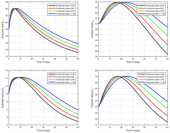
Figure 1. Time series analysis of the proposed fractional system of Zika virus infection with various fractional values, i.e., $\wp =0.85,0.90,0.95,1.00$.

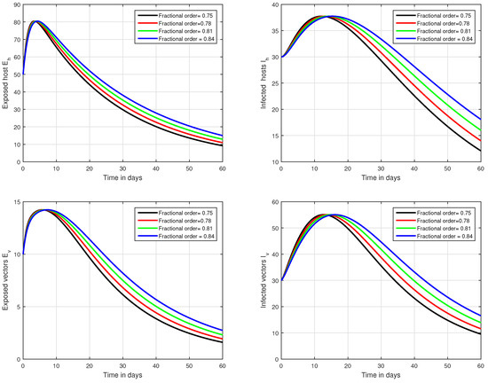
Figure 2. Graphical view analysis of the solution pathways of exposed and infected classes of our fractional system of Zika virus infection with various fractional values, i.e., $\wp =0.75,0.78,0.81,0.84$.

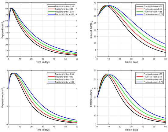
Figure 3. Graphical view analysis of the solution pathways of exposed and infected classes of our fractional system of Zika virus infection with various fractional values, i.e., $\wp =0.55,0.60,0.65,0.70$.

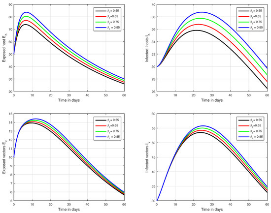
Figure 4. Graphical view analysis of the solution pathways of exposed and infected classes of our fractional system of Zika virus infection with various values of the parameter ${\beta }_1$, i.e., ${\beta }_1=0.55,0.65,0.75,0.85$.

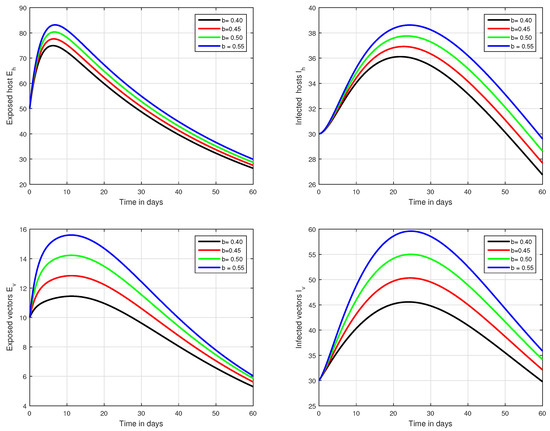
Figure 5. Graphical view analysis of the solution pathways of exposed and infected classes of our fractional system of Zika virus infection with various values of the parameter b, i.e., $b=0.40,0.45,0.55,0.60$.

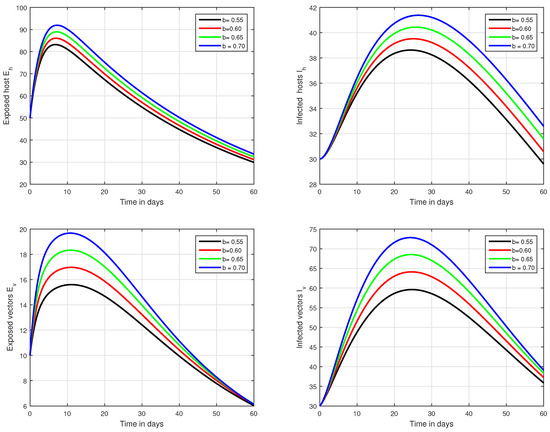
Figure 6. Illustration of the solution pathways of all the classes of our fractional model of Zika virus infection with various values of the input parameter b, i.e., $b=0.55,0.60,0.65,0.70$.

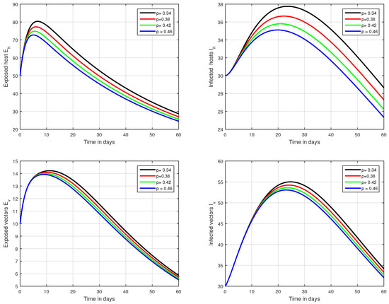
Figure 7. Illustration of the solution pathways of all the classes of our fractional model of Zika virus infection with various values of the input parameter p, i.e., $p=0.34,0.38,0.42,0.46$.

In the fifth simulation, the dynamics of Zika virus infection have been visualized with the fluctuation of the input factor d in Figure 8. This parameter can control the subsequent spread of the infection. These numerical results predicted the most important factor of the system and are recommended to the policy makers. A comparative analysis of both the operators are performed in Figure 9, Figure 10 and Figure 11, from which we noticed that the results of ABC are better than those of the CF operator.

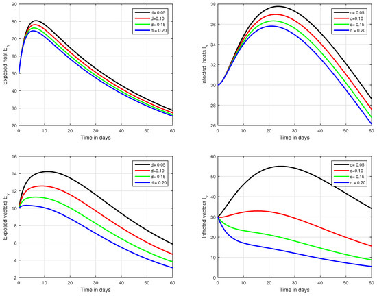
Figure 8. Illustration of the solution pathways of all the classes of our fractional model of Zika virus infection with various values of the input parameter d, i.e., $d=0.05,0.10,0.15,0.20$.

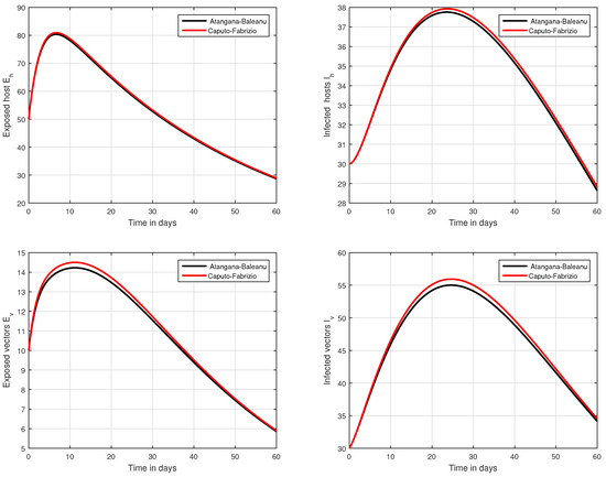
Figure 9. Comparative analysis of CF and ABC operators through the proposed model.

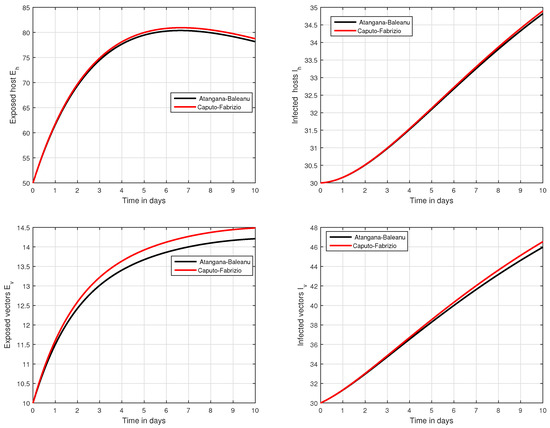
Figure 10. Time series analysis to compare the proposed CF and ABC operator.

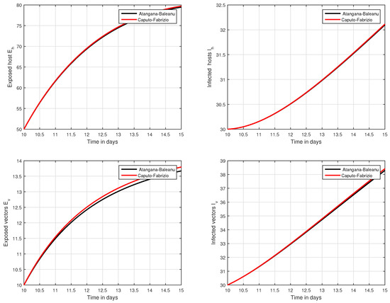
Figure 11. Time series analysis to compare the proposed CF and ABC operator from day 10 to day 15.

7. Conclusions

In this research, we have structured a compartmental model for the transmission pathway of Zika virus infection with the influence of sexual incidence rate and vaccination. We have, thus, presented the fundamental results of fractional calculus for the analysis of the proposed system of Zika virus infection. The system of Zika virus infection is interrogated through CF and ABC operators. We have further examined our system of Zika infection and determined the endemic indicator through the next-generation matrix method. The uniqueness and existence of the solution has been investigated through fixed point theory. A numerical scheme to investigate the dynamical behaviour of the system has also been constructed; hereafter, a comparison of the outcomes of the operators has been conducted. The impact of different input factor has been conceptualized through the dynamical behaviour of the system. Consequently, we have observed that lowering the fractional order parameter and decreasing sexual contact with the exposed and infected individuals are dramatically reduced. It has also been noticed that the efficacy of the vaccine is also important while the input factor b is critical. Furthermore, the impact of mosquito biting rate on infected humans has been analyzed and, based on this, control policymakers can be advised toward the point that decreasing the biting rate may greatly lower the level of Zika infection. We have shown the impact of vector control on the system and highlighted the importance of parameter d on the system as well. We have, accordingly, aimed to pave the way for future research with real datasets using fractional methods and comparisons based on the examination of our system of Zika infection and the determination of the endemic indicator through a next-generation matrix method. In the future, we also aim this scheme through comparative methods so that the most optimal models will be attained for related complex diseases.

References

- Jan, R.; Khan, M.A.; Gomez-Aguilar, J.F. Asymptomatic carriers in transmission dynamics of dengue with control interventions. Optim. Control Appl. Methods 2020, 41, 430–447. [Google Scholar] [CrossRef]
- Jan, R.; Xiao, Y. Effect of partial immunity on transmission dynamics of dengue disease with optimal control. Math. Methods Appl. Sci. 2019, 42, 1967–1983. [Google Scholar] [CrossRef]
- Jan, R.; Xiao, Y. Effect of pulse vaccination on dynamics of dengue with periodic transmission functions. Adv. Differ. Equ. 2019, 2019, 1–17. [Google Scholar] [CrossRef]
- Agusto, F.B.; Bewick, S.; Fagan, W.F. Mathematical model of Zika virus with vertical transmission. Infect. Dis. Model. 2017, 2, 244–267. [Google Scholar] [CrossRef]
- Bearcroft, W.G.C. Zika virus infection experimentally induced in a human volunteer. Trans. R. Soc. Trop. Med. Hyg. 1956, 50, 442–448. [Google Scholar] [CrossRef]
- Bonyah, E.; Khan, M.A.; Okosun, K.O.; Islam, S. A theoretical model for Zika virus transmission. PLoS ONE 2017, 12, e0185540. [Google Scholar] [CrossRef] [PubMed]
- Sulaiman, I.M.; Mamat, M.; Umar, A.; Kamfa, K.; Madi, E.N. Some Three-Term Conjugate Gradient Algorithms with Descent Condition for Unconstrained Optimization Models. J. Adv. Res. Dyn. Control Syst. 2020, 12, 2494–2501. [Google Scholar]
- Madi, E.N.; Yusoff, B. Modelling Perceptive-Based Information (Words) for Decision Support System. Int. J. Recent Technol. Eng. 2019, 7, 1–7. [Google Scholar]
- Samsudin, M.S.; Azid, A.; Abd Rani, N.L.; Mohd, K.; Yusof, K.K.; Shaharudin, S.M.; Yunus, K.; Razik, M.A.; Sidik, M.H.; Rozar, N.M. Evidence of recovery from the restriction movement order by mann kendall during the COVID-19 pandemic in malaysia. J. Sustain. Sci. Manag. 2021, 16, 55–69. [Google Scholar] [CrossRef]
- Rahi, S.; Khan, M.M.; Alghizzawi, M. Factors influencing the adoption of telemedicine health services during COVID-19 pandemic crisis: An integrative research model. Enterp. Inf. Syst. 2021, 15, 769–793. [Google Scholar] [CrossRef]
- Shah, N.H.; Patel, Z.A.; Yeolekar, B.M. Preventions and controls on congenital transmissions of Zika: Mathematical analysis. Appl. Math. 2017, 8, 500. [Google Scholar] [CrossRef][Green Version]
- Imran, M.; Usman, M.; Dur-e-Ahmad, M.; Khan, A. Transmission dynamics of Zika fever: A SEIR based model. Differ. Equ. Dyn. Syst. 2021, 29, 463–486. [Google Scholar] [CrossRef]
- Alizadeh, S.; Baleanu, D.; Rezapour, S. Analyzing transient response of the parallel RCL circuit by using the Caputo-Fabrizio fractional derivative. Adv. Differ. Equ. 2020, 2020, 1–19. [Google Scholar] [CrossRef]
- Aydogan, M.S.; Baleanu, D.; Mousalou, A.; Rezapour, S. On high order fractional integro-differential equations including the Caputo-Fabrizio derivative. Bound. Value Probl. 2018, 2018, 1–15. [Google Scholar] [CrossRef]
- Srivastava, H.M.; Jan, R.; Jan, A.; Deebani, W.; Shutaywi, M. Fractional-calculus analysis of the transmission dynamics of the dengue infection. Chaos Interdiscip. J. Nonlinear Sci. 2021, 31, 053130. [Google Scholar] [CrossRef]
- Jan, A.; Jan, R.; Khan, H.; Zobaer, M.S.; Shah, R. Fractional-order dynamics of Rift Valley fever in ruminant host with vaccination. Commun. Math. Biol. Neurosci. 2020, 2020, 79. [Google Scholar]
- Ma, C.Y.; Shiri, B.; Wu, G.C.; Baleanu, D. New fractional signal smoothing equations with short memory and variable order. Optik 2020, 218, 164507. [Google Scholar] [CrossRef]
- Kumar, D.; Singh, J.; Baleanu, D. On the analysis of vibration equation involving a fractional derivative with Mittag-Leffler law. Math. Methods Appl. Sci. 2020, 43, 443–457. [Google Scholar] [CrossRef]
- Jan, R.; Khan, M.A.; Kumam, P.; Thounthong, P. Modeling the transmission of dengue infection through fractional derivatives. Chaos Solitons Fractals 2019, 127, 189–216. [Google Scholar] [CrossRef]
- Fatmawati, F.; Jan, R.; Khan, M.A.; Khan, Y.; Ullah, S. A new model of dengue fever in terms of fractional derivative. Math. Biosci. Eng. MBE 2020, 17, 5267–5287. [Google Scholar] [CrossRef]
- Shah, Z.; Jan, R.; Kumam, P.; Deebani, W.; Shutaywi, M. Fractional Dynamics of HIV with Source Term for the Supply of New CD4+ T-Cells Depending on the Viral Load via Caputo-Fabrizio Derivative. Molecules 2021, 26, 1806. [Google Scholar] [CrossRef]
- Qureshi, S.; Jan, R. Modeling of measles epidemic with optimized fractional order under Caputo differential operator. Chaos Solitons Fractals 2021, 145, 110766. [Google Scholar] [CrossRef]
- Jan, R.; Jan, A. MSGDTM for solution of fractional order dengue disease model. Int. J. Sci. Res. 2017, 6, 1140–1144. [Google Scholar]
- Tang, T.Q.; Shah, Z.; Jan, R.; Deebani, W.; Shutaywi, M. A robust study to conceptualize the interactions of CD4+ T-cells and human immunodeficiency virus via fractional-calculus. Phys. Scr. 2021, 96, 125231. [Google Scholar] [CrossRef]
- ur Rahman, M.; Arfan, M.; Shah, K.; Gomez-Aguilar, J.F. Investigating a nonlinear dynamical model of COVID-19 disease under fuzzy caputo, random and ABC fractional order derivative. Chaos Solitons Fractals 2020, 140, 110232. [Google Scholar] [CrossRef] [PubMed]
- Jan, R.; Khan, H.; Kumam, P.; Tchier, F.; Shah, R.; Bin Jebreen, H. The Investigation of the Fractional-View Dynamics of Helmholtz Equations Within Caputo Operator. CMC Comput. Mater. Contin. 2021, 68, 3185–3201. [Google Scholar] [CrossRef]
- Qureshi, S.; Yusuf, A.; Shaikh, A.A.; Inc, M.; Baleanu, D. Fractional modeling of blood ethanol concentration system with real data application. Chaos Interdiscip. J. Nonlinear Sci. 2019, 29, 013143. [Google Scholar] [CrossRef]
- Caputo, M.; Fabrizio, M. A new definition of fractional derivative without singular kernel. Progr. Fract. Differ. Appl. 2015, 1, 1–13. [Google Scholar]
- Losada, J.; Nieto, J.J. Properties of a new fractional derivative without singular kernel. Progr. Fract. Differ. Appl. 2015, 1, 87–92. [Google Scholar]
- Atangana, A.; Baleanu, D. New fractional derivatives with nonlocal and non-singular kernel: Theory and application to heat transfer model. arXiv 2016, arXiv:1602.03408. [Google Scholar] [CrossRef]
- Castillo-Chavez, C.; Feng, Z.; Huang, W. On the computation of R0 and its role in global stability. IMA Vol. Math. Its Appl. 2002, 125, 229–250. [Google Scholar]
- Heesterbeek, J.A.P. A brief history of R0 and a recipe for its calculation. Acta Biotheor. 2002, 50, 189–204. [Google Scholar] [CrossRef] [PubMed]
- Heffernan, J.M.; Smith, R.J.; Wahl, L.M. Perspectives on the basic reproductive ratio. J. R. Soc. Interface 2005, 2, 281–293. [Google Scholar] [CrossRef] [PubMed]
Publisher’s Note: MDPI stays neutral with regard to jurisdictional claims in published maps and institutional affiliations. |
© 2021 by the authors. Licensee MDPI, Basel, Switzerland. This article is an open access article distributed under the terms and conditions of the Creative Commons Attribution (CC BY) license (https://creativecommons.org/licenses/by/4.0/).