Article

Analysis of the Influences of Parameters in the Fractional Second-Grade Fluid Dynamics

1
Department of Mathematics and Computer Sciences, Faculty of Science, Necmettin Erbakan University, 42090 Konya, Turkey
2
Department of Mathematics, College of Engineering, Mathematics and Physical Sciences, University of Exeter, Cornwall TR10 9FE, UK
3
Department of Mathematics, Institut des Politiques Publiques, Dakar Fann BP 5683, Senegal
4
Department of Mathematics, Faculty of Arts and Sciences, Bülent Ecevit University, Incivez, 67100 Zonguldak, Turkey
*
Authors to whom correspondence should be addressed.
Mathematics 2022, 10(7), 1125; https://doi.org/10.3390/math10071125
Submission received: 3 March 2022 / Revised: 28 March 2022 / Accepted: 29 March 2022 / Published: 1 April 2022

Abstract

:
This work proposes a qualitative study for the fractional second-grade fluid described by a fractional operator. The classical Caputo fractional operator is used in the investigations. The exact analytical solutions of the constructed problems for the proposed model are determined by using the Laplace transform method, which particularly includes the Laplace transform of the Caputo derivative. The impact of the used fractional operator is presented; especially, the acceleration effect is noticed in the paper. The parameters’ influences are focused on the dynamics such as the Prandtl number ( P r ) , the Grashof numbers ( G r ) , and the parameter η when the fractional-order derivative is used in modeling the second-grade fluid model. Their impacts are also analyzed from a physical point of view besides mathematical calculations. The impact of the fractional parameter α is also provided. Finally, it is concluded that the graphical representations support the theoretical observations of the paper.

1. Introduction

Fluid and nanofluid models have attracted many researchers in recent years. These fields of mathematical physics continue to increase and to be used in many domains of science as: physics, oceanography, industry, and engineering, heating process, cooling process, thermal insulation, repositories for nuclear waste, extraction of petroleum, thermal equipment, and many other domains [1,2,3,4,5]. We are interested in introducing the fractional operator to the second-grade fluid models and investigating the analytical solutions. The fractional concept operator starts with the Leibniz question, which received many answers where the Caputo derivative [6,7,8] and Riemann–Liouville derivative [6,7,8] have been proposed. All previous derivative operators answer to the Leibniz question, but the Riemann–Liouville derivative (RLD) does not provide zero when the function is a constant. This particular inconvenience of the RLD motivated the introduction of the Caputo derivative. The presence of the singularity in these classical derivatives has inspired Atangana, Baleanu, Caputo, and Fabrizio to propose new categories of fractional operators called the fractional derivatives (FDs) with an exponential kernel [9] and FDs with the Mittag–Leffler kernel [10,11,12]. There exist in the literature many papers addressing the fractional operators in modeling fluids and nanofluid models. For further investigations, one can visit the results given in [13,14,15,16,17,18]. In the present study, determining the exact analytical solutions of the fluid models interests us. In our modeling, the Caputo derivative is preferred to the other fractional operators due to the reasons previously explained and notably by its compatibility with the initial conditions that can be considered in the physical mean. In this context, there are a number of illustrative and novel applications of the fractional derivatives in physics [19,20], in mathematical biology in [21,22,23,24,25], in mathematical physics [26,27,28], in chaos theory [29,30,31], in synchronization [32], in mathematical problems [33], and many others [34,35].
The solutions of the FDEs and fluid models are open problems. Many methods to determine the analytical solutions of fluid models exist in the literature, and the more frequently used way is the Laplace transform. Vieru et al. [13] introduced the Laplace Transform (LT) method to provide analytical solutions of the temperature, concentration, and velocity of heat and mass transfer from the plate to the fluid. The investigations by Vieru et al. constituted the first explorations of this form in fractional calculus. They also utilized the Mittag–Leffler function (MLF) and Wright function in expressing the analytical solutions. In [36], Saqib et al. have applied the derivative with Mittag-Leffler kernel to (Magnetohydrodynamics) MHD channel flow of Carboxy–Methyl–Cellulose (CMC) based Carbon nanotubes (CNT’s) nanofluid through a porous medium.
In [37], the authors introduced fractional operators to MHD free convection flow of generalized Walters’-B fluid model. As described above, analytical solutions have also been proposed for the constructive equations. In [38], Sene proposed a numerical method for getting solutions of the constructive equations to free convection flows of the Casson fluid along with heat and mass transfer represented by the Caputo operator. The author used the Adams–Bashforth procedure to give discretizations of the constructive equations.
In [39], Abro et al. proposed analytical investigations of constructive equations of the fluid models using Laplace transform. See integral balance methods for getting solutions of the second-grade fluid model in [40,41]. For the other method used to get the dynamics of the fluid models, we can refer to the numerical methods; the homotopy method is frequent in nanofluid modeling. We can also find in the literature the application of the Fourier and sine transformation method. In this paper, a particular fluid model is considered. The problem to be solved consists of considering the constructive equations for the second-grade fluid model, applying the Laplace transform method in order to get the exact analytical solution. Note that, for the application of the Laplace transform method in [13] and in this paper, there is no difference in the methodology. However, we provide additional information observing that there is a difference in the initial and boundaries conditions between the investigation in [13] and the present paper. Note that the fluid models are sensitive to the modifications on the initial and boundaries conditions, this sensitivity appears in the application of the Laplace transform because this transformation depends strongly on the initial conditions. Therefore, changing initial conditions generates changes in the exact analytical solution and changes in the dynamics of the model. The advantages of the Laplace transform method lead us to use it in our examinations. In most constructive equations used in fluid models, we obtain a new second-order differential equations with or without second member when the Laplace transform is applied. To the best of our knowledge, solving second-order linear differential equations is not considered hard in general. The second advantage of the Laplace transform method used in this paper is that the exact analytical solutions are obtained and expressed using an exponential function, Gaussian error function, and Wright function. These functions are beneficial and straightforward to be implemented via MATLAB software to draw the graphical representations of the fluid dynamics model.
This paper is structured as follows. In Section 2 we give the constructive equations of the second-grade fluid model by introducing the Caputo derivative in the modeling. In Section 3, the procedure to obtain the solution via Laplace transform is presented. In Section 4, the graphical representations are proposed to support the findings of the paper. The influences of the fractional operators and the parameters of the model are also analyzed in this section. The final remarks and conclusion are given in Section 5. Finally, in Appendix A, we recall the fractional operators and all functions, which are used to express the analytical solutions throughout the paper.

2. Constructive Equations

This section is devoted to present the procedure of modeling adopted in the present paper. As described in a previous article in the literature [13], we use the same method in the modeling. The slight difference here is the use of the fractional operator. Let an incompressible second grade fluid over an infinite vertical flat plate. Let x-axis normal to the plane of the plate. At the initial time, we suppose that the fluid and the plate are at rest and at a temperature denoted by T . At the right neighborhood of the initial time, we assume that the plate begins to move at x direction with the constant velocity U 0 . Furthermore, we suppose the temperature of the fluid to be maintained at constant temperature represented in our modeling by T w for all the processes of the diffusion. The last step consists of using the usual Boussinesq approximation of temperature gradient, and therefore, our constructive equations in this paper, including the Caputo derivative, will be given by
ρ D c α u = μ 2 u x 2 + α 1 D c α 2 u x 2 + g β ρ T T ,
and
ρ c p D c α T = κ ν 2 T x 2 ,
where the term u denotes the velocity of the fluid, and T is the temperature distribution of the fluid. For simplification in the terminology, the parameters of the model are summarized in the following Table 1 with the associated units. The initial conditions of the above constructive equations can be described as the following forms, with the initial conditions given for x 0 by
u ( x , 0 ) = 0 ,
T ( x , 0 ) = T .
and as boundary conditions the following relationship is considered for our model
u ( 0 , t ) = U 0 ,
T ( 0 , t ) = T w .
It is important to mention that the order of the Caputo derivative in Equations (1) and (2) satisfies the condition α ( 0 , 1 ) . In the present investigations, the conditions are under consideration of α ( 0 , 1 ) as well. Note that the classical model of our considered model is recovered when the order of the Caputo derivative converges to 1, that is α = 1 .
In order to simplify the constructive equations of our fluid model, we consider the following variable changes known in the literature as non-dimensional quantities; then we have that
x * = x ν / U 0 , w * = u U 0 , τ * = t ν / U 0 2 , v * = T T T w T .
To obtain the constructive equations of this paper, which we will consider for the rest of the investigations, we use the variables described in Equation (7); therefore, we obtain the following constructive equations described by
D c α w = 2 w x 2 + η D c α 2 w x 2 + G r v ,
and
D c α v = 1 P r 2 v x 2 ,
with the initial conditions given by
w ( x , 0 ) = v ( x , 0 ) = 0 .
The velocity w and the temperature v get as boundary conditions the following relation
w ( 0 , τ ) = v ( 0 , τ ) = 1 .
Moreover, the Prandtl number, the Grashof number and the Casson parameter are considered as the following, respectively [42]:
P r = ν ρ c p κ = μ c p κ , G r = ν g β T w T U 0 3 , η = α 1 U 0 2 μ ν .
Let us now develop the novelty of the present investigations. At first, we use the Caputo derivative in the modeling to take into account the accumulation of the memory effects and analyze its influence on the dynamics of the fluid model. The second point on which we attract the readers is the initial conditions. The initial conditions considered in our modeling are compatible with the Caputo derivative, but not, for example, with the Riemann–Liouville derivative, which has the initial condition in an integral form that can not be interpreted physically. We can observe that the initial conditions and boundary conditions in Equations (10) and (11) are not frequent in the literature. Therefore, it will be interesting to get the solution when these initial and boundary conditions are used. The other main importance of writing this paper is that we want to determine the exact analytical solutions of model (8) and (9) by using the LTs, including the LT of the Caputo derivative. The last importance of the present investigations is to know the impacts of the parameters of the model (8) and (9) described in Table 1.

3. Solution Procedures

In this section, we propose the analytical solutions of the model described at Equations (8) and (9) by considering the initial and boundary conditions described at Equations (10) and (11). We particularly use the Laplace transform method. We divided this section into two parts. In the first section, we determine the exact analytical solution of the fractional heat equation, and in the second part, we propose the analytical form of the velocity.

3.1. Fractional Heat Equation

In this section, we consider the fractional diffusion equation described by Equation (9). For the simplicity, we recall again the differential equation represented by the Caputo derivative given by
D c α v = 1 P r 2 v x 2 .
Firstly, the resolution procedure consists of applying the Laplace transform; the present application of the Laplace transform of the Caputo derivative, which is given in Equation (A3) in Appendix A, can be considered as a novelty of the paper. After application of the Laplace transform according to time variable, we observe that we can obtain a classical differential equation that is not difficult to solve. Note that using the Laplace transform to Equation (13), we get the following relationship
s α v ¯ s α 1 v ( x , 0 ) = 1 P r 2 v ¯ x 2 , 2 v ¯ x 2 P r s α v ¯ = 0 .
We recognize that Equation (14) is a classical second-order differential equation that we solve by considering the Laplace transform of the initial condition described as the form ϕ ¯ ( 0 , s ) = 1 s . The solution of the homogeneous equation can be represented classically by the following form
v ¯ ( x , s ) = A exp x s α P r + B exp x s α P r .
The exact analytical solution of Equation (14) under the initial condition previously mentioned can be represented as the following form
v ¯ ( x , s ) = 1 s exp x s α P r = 1 s exp x P r s α / 2 .
For the inverse of the Laplace transform of Equation (16), we use the Tzou algorithm described in the following expression, we have that
v ( x , τ ) = e 4.7 τ 1 2 v ¯ ( x , 4.7 τ ) + R e k = 1 N 1 1 k v ¯ ( x , 4.7 + k π i τ ) ,
where R e ( ) designs the real part of the complex number, i is the imaginary unit, and N 1 is a natural number. Equation (17) is the Tzou formula provided to obtain the inverse of the Laplace transform for heat equations [43]. According to the source paper [43], Equation (17) is Riemann sum approximation, and then a series representation is used, thus the convergence of the series is needed. As reported in [43] the value 4.7 ensures the fast convergence of the series representation. The second remark is to give explanations about N 1 that contributes to the convergence and can be chosen approximately as 18 for effective analytical solutions for the heat equations [43].
We continue to this procedure by describing the solution for a special case when the order of the Caputo derivative converges to 1. For clarity and for the young readers to reproduce the present investigations, we repeat the previous procedure with α = 1 . The Laplace transform in the context of integer order derivative with our constructive equation is given by the following form:
s v ¯ v ( x , 0 ) = 1 P r 2 v ¯ x 2 , 2 v ¯ x 2 P r s v ¯ = 0 .
The resolution of this second differential equation with the initial condition ϕ ¯ ( 0 , s ) = 1 s provide the following solution:
v ¯ ( x , s ) = 1 s exp x s P r .
For the Laplace transform of Equation (19), to obtain the exact analytical solution, we replace Equation (19) in Equation (17).
A comparative study can be done in this part. The authors in [44] proposed the exact solution via the use of the Laplace transform for the fractional wave equation where the order of the Caputo derivative satisfies the condition that α ( 1 , 2 ) . The difference between the present investigations and the investigations in [44] is that the authors in [44] have applied the Laplace transform and the Fourier transformations to get the exact solution. The second difference between the investigations which is very important is that in the present works the order of the Caputo derivative verifies the condition that α ( 0 , 1 ) .

3.2. The Velocity Profile

In this section, we consider Equation (8) with the initial and boundary conditions defined in Equations (10) and (11). For more clarity in the reasoning, we recall the equation under consideration given as the following form:
D c α w = 2 w x 2 + η D c α 2 w x 2 + G r v .
Applying the Laplace transform to Equation (20) and taking into account that the Laplace transform of fractional derivative of diffusion term, which should contain a term with the initial condition of zero referring to Equation (10), we get the following equation to solve:
s α w ¯ s α 1 w ( x , 0 ) = 2 w ¯ x 2 + η s α 2 w ¯ x 2 + G r v ¯ , G r s exp x s α P r = 1 + η s α 2 w ¯ x 2 s α w ¯ .
For simplification, we multiply Equation (21) by the constant 1 / ( 1 + η s α ) ; then we get the following relationship:
2 w ¯ x 2 s α 1 + η s α w ¯ = G r s 1 + η s α exp x s α P r .
The main objective now is to solve the second-order differential equation with an initial statement given by the form w ¯ ( 0 , s ) = 1 s . For more clarity, we solve the equation using a classical procedure. The solution of the homogeneous equation can be represented as the following form:
w ¯ h ( x , s ) = A exp x s α 1 + η s α + B exp x s α 1 + η s α .
We now solve the complete equation represented in Equation (22); the particular solution satisfies the following form:
w ¯ p ( x , s ) = C exp x s α P r .
The objective here is to get the form of the constant C . After calculation and simplification, we get the following form for the particular solution:
w ¯ p ( x , s ) = G r s α P r η s α + P r 1 exp x s α P r s .
Considering the LT of the initial condition (IC), the complete solution of Equation (22) can be represented as the following form:
w ¯ = 1 s exp x s α 1 + η s α + G r s α P r η s α + P r 1 1 s exp x s α 1 + η s α G r s α P r η s α + P r 1 exp x s α P r s .
The inverse Laplace transform (ILT) of Equation (26) can be obtained by Tzou algorithm described in the following representation:
w ( x , τ ) = e 4.7 τ 1 2 w ¯ ( x , 4.7 τ ) + R e k = 1 N 1 1 k w ¯ ( x , 4.7 + k π i τ ) .
We finish by focusing on the limiting cases in terms of the present model (8) and (9). We repeat the same procedure of getting the velocity by applying the Laplace transform in the context of the integer-order derivative. For the first limiting case, we suppose that η = 0 and α = 1 , the Laplace transform of Equation (20) give the following form:
s w ¯ w ( x , 0 ) = 2 w ¯ x 2 + G r v ¯ , G r s exp x s P r = 2 w ¯ x 2 s w ¯ .
After a simple calculation, the solution of Equation (28) can be expressed as the following form:
w ¯ ( x , s ) = 1 s exp x s + G r ( P r 1 ) s exp x s s + G r ( 1 P r ) s exp x s P r s .
For the Laplace transform of Equation (29), to obtain the exact analytical solution, we replace Equation (29) in Equation (27).
We continue proposing a solution with another particular case that is obtained when the order α = 1 . There are no other constraints on the parameters of the model. The application of the Laplace transform and taking into account that the Laplace transform of fractional derivative of diffusion term, which should contain a term with the initial condition is zero referring to Equation (10), we obtain the following equation to solve:
s w ¯ w ( x , 0 ) = 2 w ¯ x 2 + η s 2 w ¯ x 2 + G r v ¯ , 2 w ¯ x 2 s 1 + η s w ¯ = G r s 1 + η s exp x s P r .
The solution of the Equation (30) can be represented as the following form; we have the following representations:
w ¯ = 1 s exp x s 1 + η s + G r s P r η s + P r 1 1 s exp x s 1 + η s G r s P r η s + P r 1 exp x s P r s .
By the same procedure as in the previous part is adopted, the inverse of Equation (31) can be obtained by Tzou algorithm described in the following representation:
w ( x , τ ) = e 4.7 τ 1 2 w ¯ ( x , 4.7 τ ) + R e k = 1 N 1 1 k w ¯ ( x , 4.7 + k π i τ ) .
Two important numbers will be determined: One of them is the Nusselt number obtained via temperature distribution and the other one is the skin friction number obtained via the temperature distribution. Note that the Nusselt number is a local number which measures the rate of heat transfer from the plate to the considered fluid. In the present section, these numbers will be assigned in tables and will be analyzed mathematically. For the Nusselt number, the values are obtained via the following formula:
N u = L 1 lim x 0 v ¯ x , s x = P r τ α / 2 Γ 1 α / 2 .
The inverse of the Laplace transform is applied according to the second variable “s” which is the variable of the Laplace transform, then its inverse should depend on the time here represented by τ after the introduction of the changes variables in Equation (7). Here, the unit is not specified for N u , see Vieru et al. [13,45] for more information.

4. Results and Discussions

In this section, we develop the graphical representations of the dynamics of the fractional heat equation and the first equation of the model described in Equations (8) and (9). Many points are analyzed in this section and illustrated by the graphics. Firstly, we examine the influence of the fractional-order derivative in the model dynamics at different times. Then, we consider analyzing the Prandtl number P r in the fractional heat equation and the velocity distribution and we explain the reason of the behaviors. After that, the Grashof number G r is also studied in the first equation of our fractional model and the dynamics at different times in terms of physical view points. The influence of the parameter η behind the Caputo derivative is also explored. All results that are necessary for the future investigations will be focused on in this section.
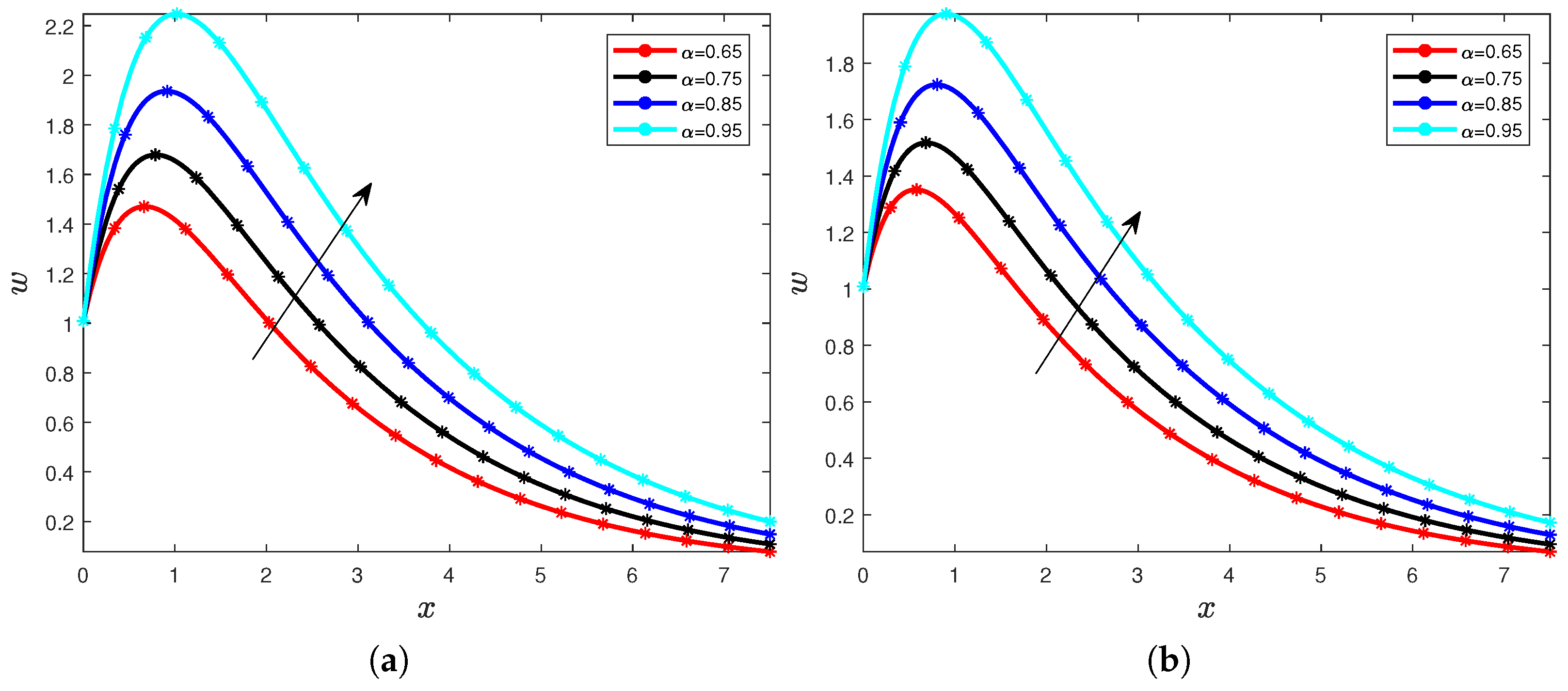
We begin the figures with the velocity distribution. To analyze the influence of the order of the fractional operators, we take into account the following values for the Prandtl number P r = 5 ; 10 ; 15 ; 20 , G r = 5 , η = 0.5 and the time τ = 10 . We consider different values of the order of fractional operators as described in the following Figure 1a,b and Figure 2a,b. We notice that when the order of the fractional operator increases, then the order of the velocity distribution increases too. We also notice with a careful comparison between Figure 1a,b and Figure 2a,b the increase of the Prandtl number in the velocity generates a decrease in the velocity. These dynamics can be explained by the fact that the diffusivity is reduced in the temperature departure distribution, which impacts the velocity referencing to the constructive equations.
The second part will be to analyze the Grashof number G r in the velocity distributions, for that we fix the following assumptions that are P r = 5 , α = 0.65 ; 0.75 ; 0.85 ; 0.95 , η = 0.5 and the time τ = 10 . We consider different values for the Grashof number G r .
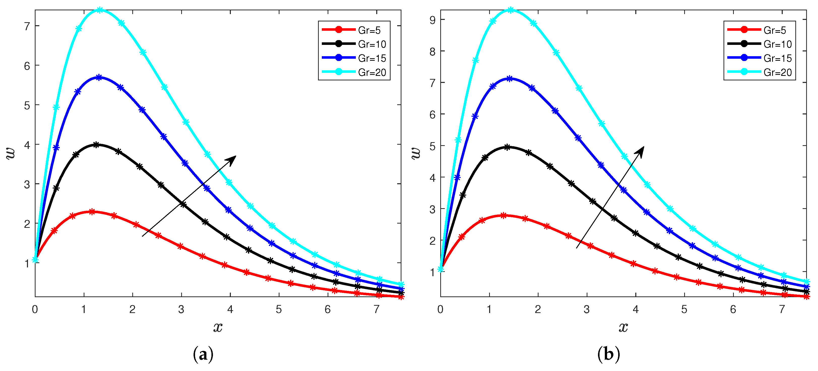
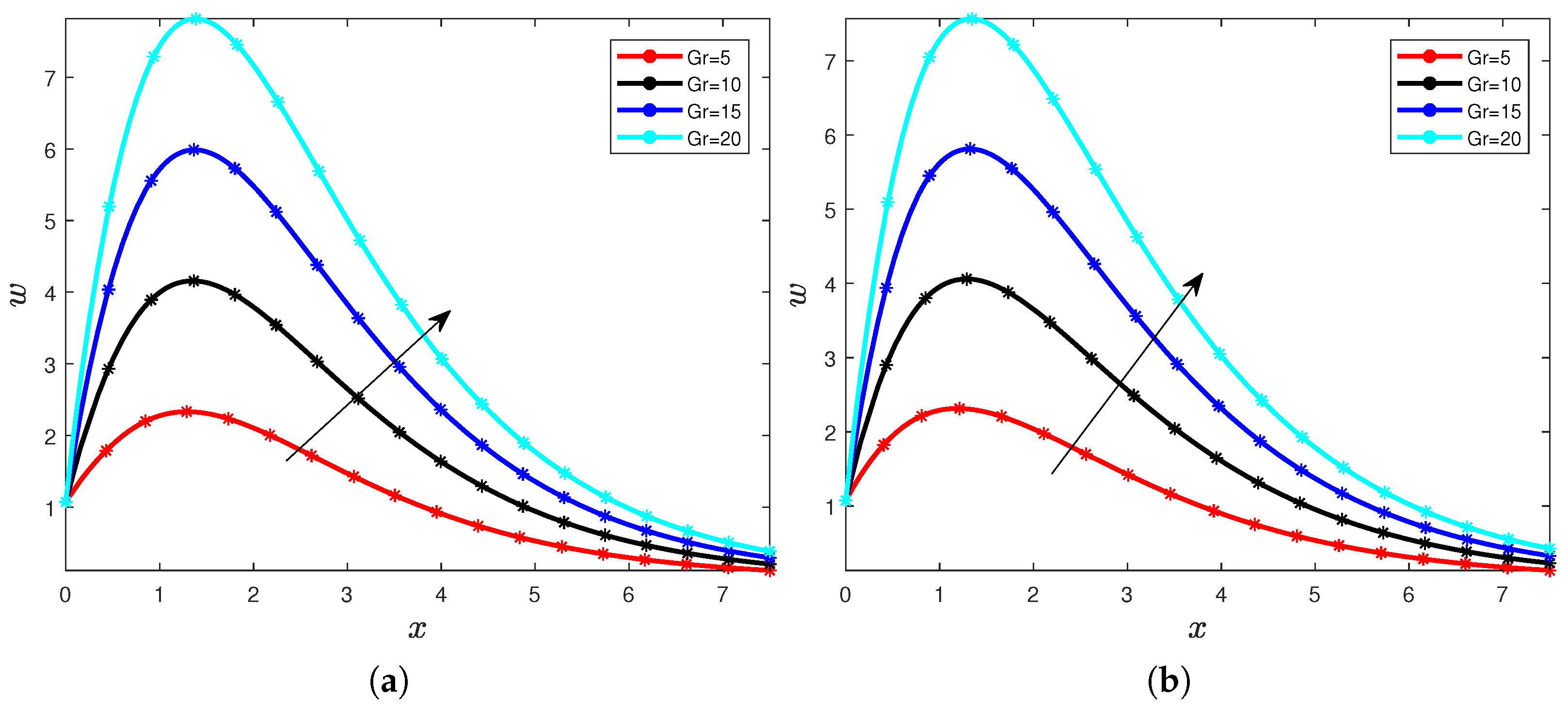
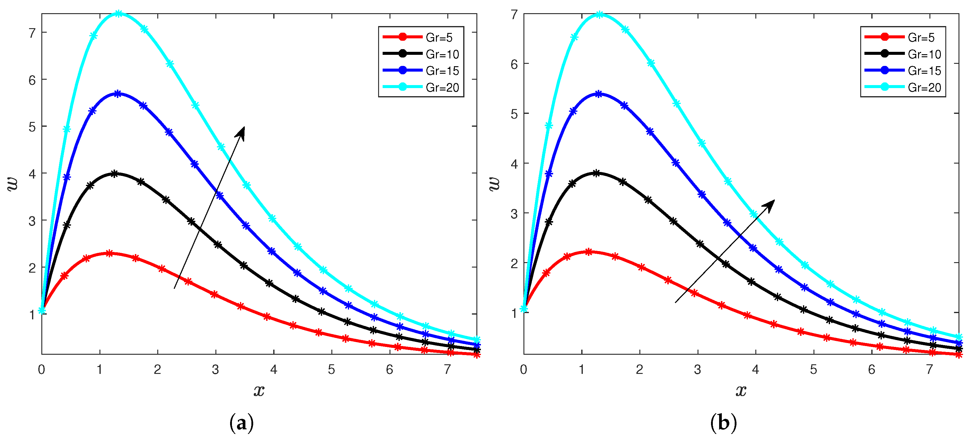
Using Figure 3a,b and Figure 4a,b, we can fix the following. We notice the increase in the value of Grashof number G r causes the increase of the velocity distributions, it is because with the increase of the Grashof number G r and the increase of the fractional-order derivative. This behavior can be described by the rise in G r number and the fractional order derivative generating the so-called buoyancy forces and the accumulation of the memory and then its increase generates the increase of the velocity. We continue with the analysis with the Casson parameter η in the dynamics. We fix that number in the dimensionless model P r = 5 , G r = 5 ; 10 ; 15 ; 20 , η = 0 ; 0.3 ; 0.5 ; 1 and the time τ = 10 . Figure 5a,b and Figure 6a,b depict the solution for the Casson parameter values η = 0 , 0.3 , 0.5 , 1 , respectively.
The graphical representations in Figure 5a,b and Figure 6a,b give the following illustrative results: When the values of the Casson parameter increase, then the values of the velocity decrease as well. This increase can be noticed when one compares all the four figures for this paper. This decrease in the velocity distribution can be explained by the fact that when this number increases, the momentum boundary layer increases significantly and it automatically generates a reduction in the velocity.
We now past in the findings related to the temperature distribution of the considered fluid. We fix successively P r = 10 , P r = 15 , P r = 20 , and P r = 25 and we consider different values of the fractional order α . Then, we have the following graphical representations Figure 7a,b and Figure 8a,b.
The first observation with the dynamics is that when the order of the fractional derivative increases, then the profile of temperature in the fractional heat equation represented in Equation (9) increases, too. We remind that the values of the time considered also play a significant role in the increasing behaviors. This increase in the profile of temperature in the heat equation can be explained by the accumulation of the memories generated by the Caputo derivative. The increase can also be explained by the fact that when the Caputo derivative order increases, then the thickness of the thermal boundary layer increases with the rise of the time and the order of the Caputo derivative, and it generates an increase in the temperature profile.
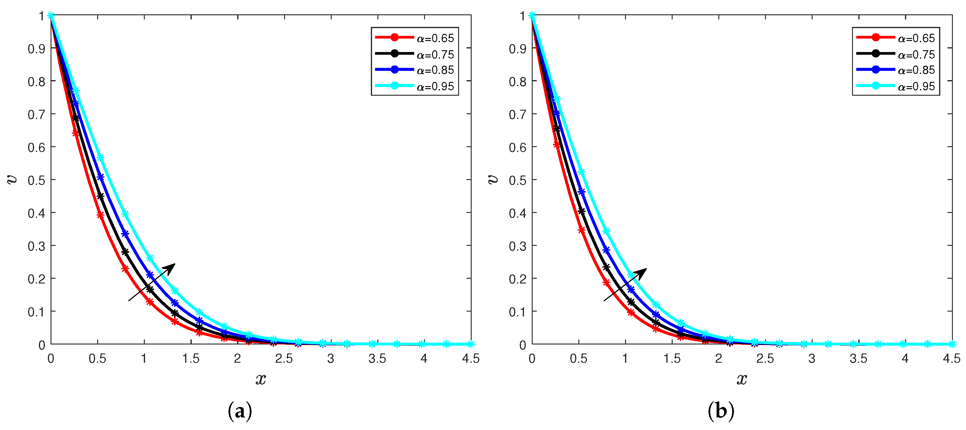
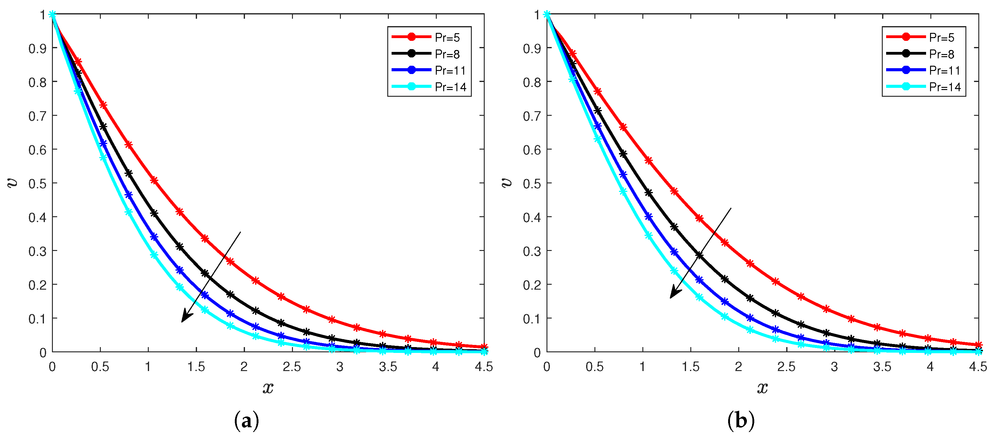
We now consider the variation of the Prandtl number P r , and we fix the order of the fractional operator. We take into account in the first graphics α = 0.65 , in the second α = 0.75 , in the third α = 0.85 and in the last α = 0.95 . We suppose time t = 10 , in all the graphics. We have the following Figure 9a,b and Figure 10a,b for more clarity.
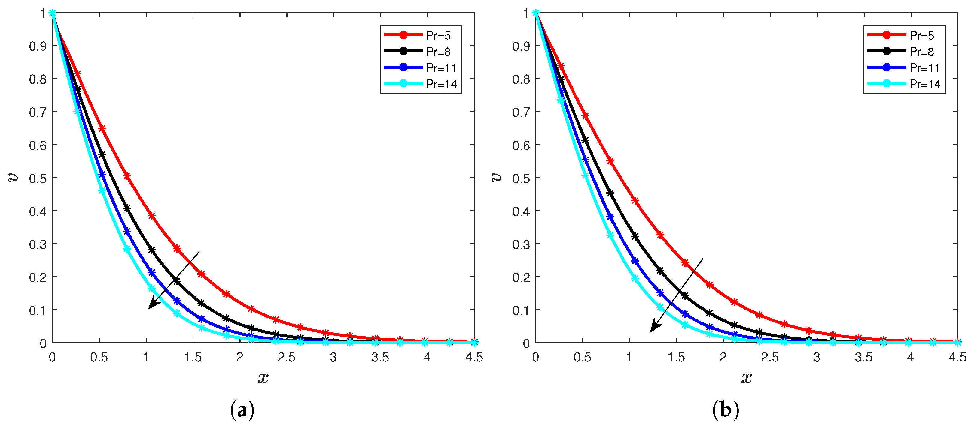
We can observe that when the Prandtl number P r increases, the temperature distribution decreases for all considered orders. The decrease is indicated by the arrow in Figure 9a,b and Figure 10a,b. These behaviors can be explained by the fact that for all considered orders of the Caputo derivative, when the Prandtl number P r increases, it generates a reduce in the diffusivity significantly; we notice in our context that it reduces the profile of the temperature. We can also notice the values of the time has no impact on the influence of the Prandtl number P r , we illustrate in the following Figure 11a,b and Figure 12a,b. We fix t = 5 , then we have the following Figures.
We finish this section by calculating the values of the Nusselt number according to the variation of the time and the Prandtl number, we use the inverse of the Laplace transform given for the Caputo derivative. We have the following Table 2, where we consider the order α = 0.85 .
The values in Table 2 have been calculated according to Equation (33). Let us now analyze the behavior of the Nusselt number according to the variation of the time and Prandtl number. We obtain that the increase in the Prandtl number generates the increase in the Nusselt number due to the fact that the Prandtl number reduces the divisivity of the diffusion process.
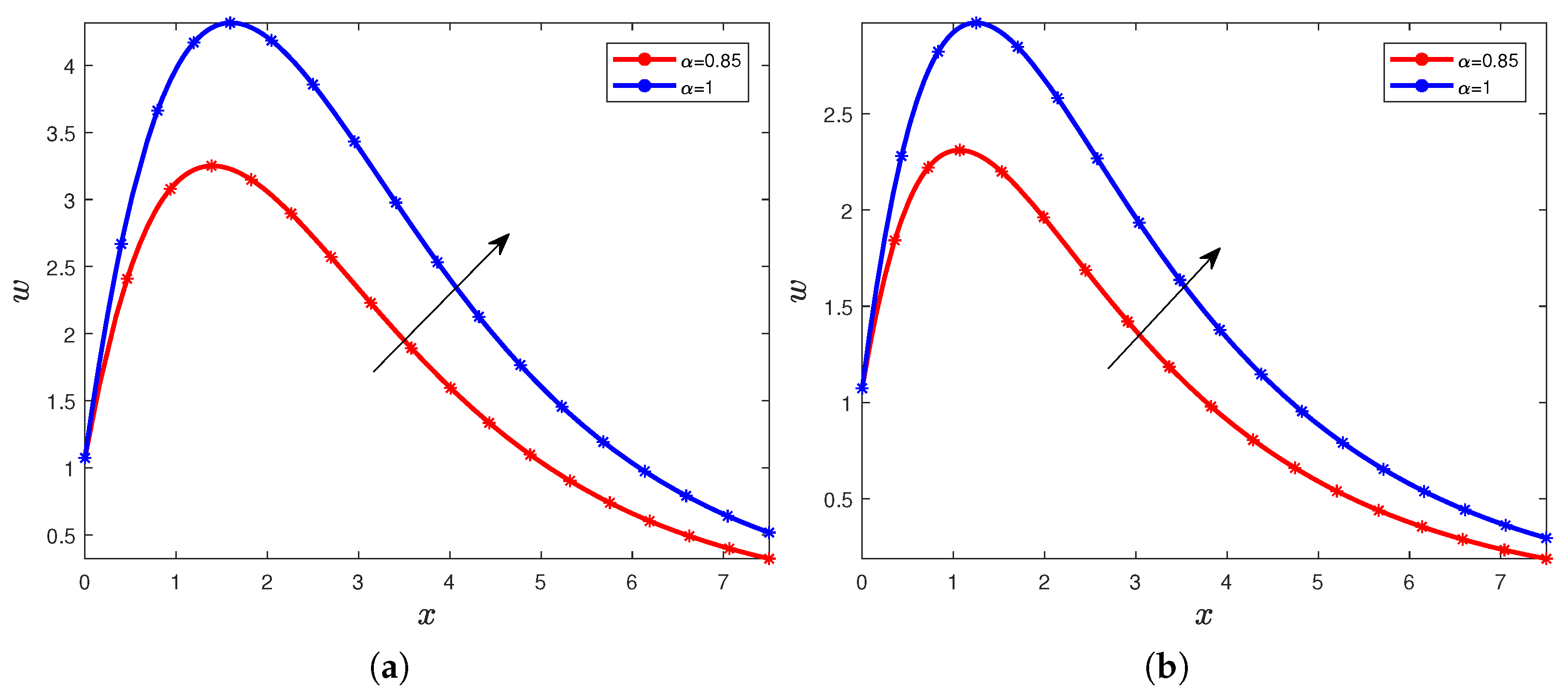
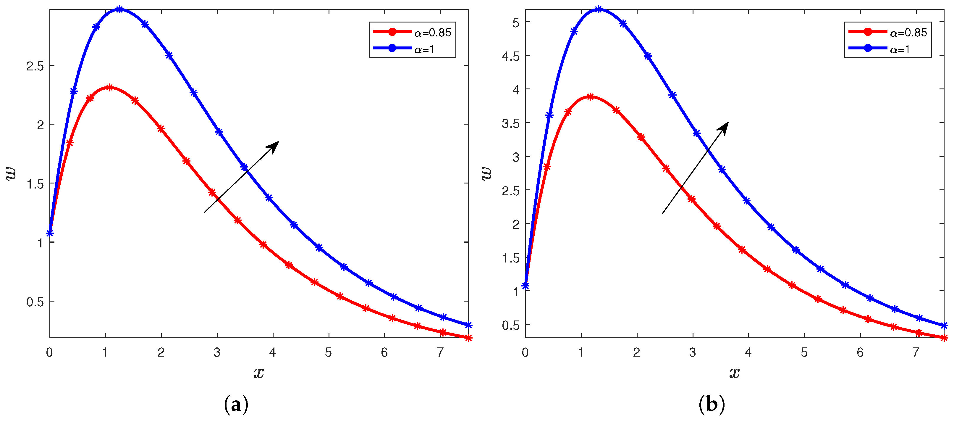
In this last part, we give a comparative study between the fractional case where the order of the Caputo derivative satisfies the condition that α 0 , 1 and the classical case where α = 1 . We work in this part with the velocity profile, the temperature follows the same findings, we have the following Figure 13a,b and Figure 14a,b. We consider that η = 1 and the time τ = 10 .
In Figure 13a,b, we fix G r = 20 . In Figure 14a,b, we have considered P r = 10 . The first remark is that in all the Figure 13a,b and Figure 14a,b, we notice the curve with the fractional order is before the curve obtained in the classical case. These behaviors and these differences in the graphics can be explained by the fact that when the order of the fractional-order derivative is into α 0 , 1 , we are in the context of the sub-diffusion process. Therefore, the behaviors of the velocity converge to the behaviors in the classical case. Note that there exist many diffusion processes: the sub-diffusion when α 0 , 1 , the super-diffusion when α 1 , 2 , the ballistic diffusion when α = 2 , and others. It is one of the advantages of the fractional-order derivative, it generates new types of diffusion processes in physics. The second remark is that the impact of the Prandtl number P r does not change, it increases generates a decrease in the velocity distribution, see Figure 13a,b. The influence of the Grashof number G r also does not vary, its increase generates an increase in the velocity as it can be observed in Figure 14a,b.

5. Conclusions

In this paper, we have considered the second-grade fluid model described by the Caputo fractional derivative. The novelties of this paper are the method used to get the solutions and studying the influences of the parameters for the considered model. Particularly, we have used the Laplace transform of the Caputo fractional-order derivative. Several particular cases have been discussed for the validation of our investigations. The main findings described in our paper can be summarized as the follows: The numbers P r and η cause a decrease in the velocity and the temperature profile. Two points may explain the reasons for this behavior: For the Prandtl number P r , it is due to the impact on the diffusivity of the system. And for the number η , it is due to the increase of the momentum boundary layer. The Grashof number G r , which appears in the modeling in Equation (8), generates an increase in the velocity when its values increase. The reason is the apparition of significant buoyancy forces. Another considerable point addressed in this paper is the influence of the fractional-order derivative, which plays an acceleration effect due to the memory effect accumulation. Time also has a significant role in the diffusion processes, which can be seen in the present paper as well.

Author Contributions

Conceptualization, M.Y. (Mehmet Yavuz) and N.S.; methodology, M.Y. (Mehmet Yavuz) and N.S.; software, N.S.; validation, M.Y. (Mehmet Yavuz), N.S. and M.Y. (Mustafa Yıldız); formal analysis, M.Y. (Mehmet Yavuz); investigation, M.Y. (Mehmet Yavuz), N.S. and M.Y. (Mustafa Yıldız); data curation, N.S.; writing—original draft preparation, M.Y. (Mehmet Yavuz) and N.S.; writing—review and editing, M.Y. (Mehmet Yavuz), N.S. and M.Y. (Mustafa Yıldız); visualization, M.Y. (Mehmet Yavuz) and N.S.; supervision, M.Y. (Mustafa Yıldız); project administration, N.S.; funding acquisition, M.Y. (Mehmet Yavuz) and M.Y. (Mustafa Yıldız). All authors have read and agreed to the published version of the manuscript.

Funding

This research received no external funding.

Institutional Review Board Statement

Not applicable.

Informed Consent Statement

Not applicable.

Data Availability Statement

Not applicable.

Conflicts of Interest

The authors declare that they have no conflict of interest.

Appendix A. Fractional Calculus Operators

The Caputo derivative, the Riemann–Liouville (RL) integral and a couple of special functions will be recalled in this section. The Caputo derivative and its Laplace transform will help us determine the exact solutions for the constructive equations of the second-grade fluid under the Newtonian fractional heat equation. Note that there exist many other types of fractional operators as the Caputo–Fabrizio derivative (CFD), the fractional-order derivative with Mittag–Leffler kernel, the conformable derivative, which may also be used in our present investigations. In this section, we begin with the fractional integral operator:
Definition A1
([7,8]). The Riemann–Liouville integral of a considered function v : [ 0 , + [ R can be described as the following form
I α v ( t ) = 1 Γ ( α ) 0 t t s α 1 v ( s ) d s ,
where Γ ( ) is the Gamma function and with the fractional order α verifying the condition that α > 0 .
After the Riemann–Liouville integral, we recall the Caputo fractional operator. Note that this fractional operator and its associated Laplace transform are used for the rest of the investigations. The reason for the utilization is that this derivative obeys the initial conditions considered in our study contrary to the Riemann–Liouville derivative, which utilizes the initial condition in an integral form that can not be interpreted physically. We have the following definition.
Definition A2
([7,8]). We describe the Caputo fractional operator for the mentioned function as:
D c α v ( t ) = 1 Γ 1 α 0 t d v d s t s α d s ,
where t > 0 , is time, the order of the fractional operator verifying the assumption that α 0 , 1 and Γ ( ) represents the Euler’s Gamma function.
The LT will play an essential role in determining the exact analytical solutions because the method applied in this paper uses the application of the Laplace transform and its inverse. The Laplace transform of the Caputo operator [7,8] can be represented as the following form
L D c α h ( t ) = s α L h ( t ) s α 1 h ( 0 ) ,
where the order α obeys to the relationship α ( 0 , 1 ) . We finish this section by recalling several special functions called Mittag–Leffler function and Wright function, which will play an important role in our investigations. We give the following definitions:
Definition A3
([13]). The Mittag–Leffler function with two parameters is defined in the following form:
E α , β z = k = 0 z k Γ ( α k + β ) ,
where α > 0 , β R and z C .
Definition A4
([13]). The Wright function with three variables is defined in the following form:
Λ β , σ , z = n = 0 z n Γ n + 1 Γ β σ n ,
where σ ( 0 , 1 ) , β R and z C .

References

  1. Lohana, B.; Abro, K.A.; Shaikh, A.W. Thermodynamical analysis of heat transfer of gravity-driven fluid flow via fractional treatment: An analytical study. J. Therm. Anal. 2021, 144, 155–165. [Google Scholar] [CrossRef]
  2. Pramanik, S. Casson fluid flow and heat transfer past an exponentially porous stretching surface in presence of thermal radiation. Ain Shams Eng. J. 2014, 5, 205–212. [Google Scholar] [CrossRef] [Green Version]
  3. Riaz, M.B.; Imran, M.A.; Shabbir, K. Analytic solutions of Oldroyd-B fluid withfractional derivatives in a circular duct that appliesa constant couple. Alex. Eng. J. 2016, 55, 3267–3275. [Google Scholar] [CrossRef] [Green Version]
  4. Imran, M.A.; Shah, N.A.; Khan, I.; Aleem, M. Applications of non-integer Caputo time fractional derivatives to natural convection flow subject to arbitrary velocity and Newtonian heating. Neural Comput. Appl. 2018, 30, 1589–1599. [Google Scholar] [CrossRef]
  5. Qureshi, S.; Yusuf, A.; Shaikh, A.A.; Inc, M.; Baleanu, D. Fractional modeling of blood ethanol concentration system with real data application. Chaos Interdiscip. J. Nonlinear Sci. 2019, 29, 013143. [Google Scholar] [CrossRef]
  6. Jarad, F.; Abdeljawad, T.; Baleanu, D. On the generalized fractional derivatives and their Caputo modification. J. Nonlinear Sci. Appl. 2017, 10, 2607–2619. [Google Scholar] [CrossRef] [Green Version]
  7. Kilbas, A.; Srivastava, H.M.; Trujillo, J.J. Theory and Applications of Fractional Differential Equations, North-Holland Mathematics Studies; Elsevier: Amsterdam, The Netherlands, 2006; p. 204. [Google Scholar]
  8. Podlubny. Fractional Differential Equations, Mathematics in Science and Engineering; Academic Press: New York, NY, USA, 1999; p. 198. [Google Scholar]
  9. Caputo, M.; Fabrizio, M. A new definition of fractional derivative without singular kernel. Progr. Fract. Differ. Appl. 2015, 1, 1–15. [Google Scholar]
  10. Atangana, A.; Mekkaoui, T. Trinition the complex number with two imaginary parts: Fractal, chaos and fractional calculus. Chaos Solitons Fractals 2019, 128, 366–381. [Google Scholar] [CrossRef]
  11. Atangana, A.; Baleanu, D. New fractional derivatives with nonlocal and non-singular kernel: Theory and application to heat transfer model. Therm. Sci. 2016, 20, 763–769. [Google Scholar] [CrossRef] [Green Version]
  12. Owolabi, K.; Atangana, A. On the formulation of Adams-Bashforth scheme with Atangana-Baleanu-Caputo fractional derivative to model chaotic problems. Chaos Interdiscip. J. Nonlinear Sci. 2019, 29, 023111. [Google Scholar] [CrossRef] [PubMed]
  13. Vieru, D.; Fetecau, C.; Fetecau, C. Time-fractional free convection flow near a vertical plate with Newtonian heating and mass diffusion. Therm. Sci. 2015, 19, 85–98. [Google Scholar] [CrossRef]
  14. Khan, A.; Abro, K.A.; Tassaddiq, A.; Khan, I. Atangana–Baleanu and Caputo Fabrizio Analysis of Fractional Derivatives for Heat and Mass Transfer of Second Grade Fluids over a Vertical Plate: A Comparative Study. Entropy 2017, 19, 279. [Google Scholar] [CrossRef] [Green Version]
  15. Khalid, A.; Khan, I.; Khan, A.; Shafie, S. Unsteady MHD free convection flow of Casson fluid past over an oscillating vertical plate embedded in a porous medium. Eng. Sci. Technol. Int. J. 2015, 18, 309–317. [Google Scholar] [CrossRef] [Green Version]
  16. Ali, F.; Sheikh, N.A.; Khan, I.; Saqib, M. Magnetic field effect on blood flow of Casson fluid in axisymmetric cylindrical tube: A fractional model. J. Magn. Magn. Mater. 2017, 423, 327–336. [Google Scholar] [CrossRef]
  17. Imran, M.; Sarwar, S. Effects of slip on free convection flow of Casson fluid over an oscillating vertical plate. Bound. Value Probl. 2016, 2016, 30. [Google Scholar] [CrossRef] [Green Version]
  18. Haq, S.U.; Jan, S.U.; Shah, S.I.A.; Khan, I.; Singh, J. Heat and mass transfer of fractional second grade fluid with slippage and ramped wall temperature using Caputo-Fabrizio fractional derivative approach. AIMS Math. 2020, 5, 3056–3088. [Google Scholar] [CrossRef]
  19. Saad, K.; Baleanu, D.; Atangana, A. New fractional derivatives applied to the Korteweg–de Vries and Korteweg–de Vries–Burger’s equations. Comput. Appl. Math. 2019, 37, 5203–5216. [Google Scholar] [CrossRef]
  20. Veeresha, P. A Numerical Approach to the Coupled Atmospheric Ocean Model Using a Fractional Operator. Math. Model. Numer. Simul. Appl. 2021, 1, 1–10. [Google Scholar] [CrossRef]
  21. Jajarmi, A.; Yusuf, A.; Baleanu, D.; Inc, M. A new fractional HRSV model and its optimal control: A non-singular operator approach. Phys. A Stat. Mech. Appl. 2020, 547, 123860. [Google Scholar] [CrossRef]
  22. Allegretti, S.; Bulai, I.M.; Marino, R.; Menandro, M.A.; Parisi, K. Vaccination effect conjoint to fraction of avoided contacts for a Sars-Cov-2 mathematical model. Math. Model. Numer. Simul. Appl. 2021, 1, 56–66. [Google Scholar] [CrossRef]
  23. Naik, P.A.; Yavuz, M.; Qureshi, S.; Zu, J.; Townley, S. Modeling and analysis of COVID-19 epidemics with treatment in fractional derivatives using real data from Pakistan. Eur. Phys. J. Plus 2020, 135, 1–42. [Google Scholar] [CrossRef] [PubMed]
  24. Wang, X.; Wang, Z. Dynamic Analysis of a Delayed Fractional-Order SIR Model with Saturated Incidence and Treatment Functio. Int. J. Bifurc. Chaos 2018, 28, 1850180. [Google Scholar] [CrossRef]
  25. Qureshi, S.; Yusuf, A.; Shaikh, A.A.; Inc, M. Transmission dynamics of varicella zoster virus modeled by classical and novel fractional operators using real statistical data. Phys. A Stat. Mech. Appl. 2019, 534, 122149. [Google Scholar] [CrossRef]
  26. Riaz, M.B.; Abro, K.A.; Abualnaja, K.M.; Akgül, A.; Rehman, A.U.; Abbas, M.; Hamed, Y.S. Exact solutions involving special functions for unsteady convective flow of magnetohydrodynamic second grade fluid with ramped conditions. Adv. Differ. Equ. 2021, 2021, 408. [Google Scholar] [CrossRef]
  27. Martínez-Farías, F.J.; Alvarado-Sánchez, A.; Rangel-Cortes, E.; Hernández-Hernández, A. Bi-dimensional crime model based on anomalous diffusion with law enforcement effect. Math. Model. Numer. Simul. Appl. 2022, 2, 26–40. [Google Scholar] [CrossRef]
  28. Kumar, D.; Singh, J.; Baleanu, D. On the analysis of vibration equation involving a fractional derivative with Mittag-Leffler law. Math. Methods Appl. Sci. 2020, 43, 443–457. [Google Scholar] [CrossRef]
  29. Gholami, M.; Ghaziani, R.K.; Eskandari, Z. Three-dimensional fractional system with the stability condition and chaos control. Math. Model. Numer. Simul. Appl. 2022, 2, 41–47. [Google Scholar] [CrossRef]
  30. Joshi, H.; Jha, B.K. Chaos of calcium diffusion in Parkinson s infectious disease model and treatment mechanism via Hilfer fractional derivative. Math. Model. Numer. Simul. Appl. 2021, 1, 84–94. [Google Scholar] [CrossRef]
  31. Sene, N. Analysis of a Four-Dimensional Hyperchaotic System Described by the Caputo–Liouville Fractional Derivative. Complexity 2020, 2020, 8889831. [Google Scholar] [CrossRef]
  32. Hammouch, Z.; Yavuz, M.; Özdemir, N. Numerical Solutions and Synchronization of a Variable-Order Fractional Chaotic System. Math. Model. Numer. Simul. Appl. 2021, 1, 11–23. [Google Scholar] [CrossRef]
  33. Fahd, J.; Abdeljawad, T. Generalized fractional derivatives and Laplace transform. Discrete Contin. Dyn. Syst.-S 2020, 13, 709. [Google Scholar]
  34. Baleanu, D.; Fernandez, A.; Akgül, A. On a Fractional Operator Combining Proportional and Classical Differintegrals. Mathematics 2020, 8, 360. [Google Scholar] [CrossRef] [Green Version]
  35. Yokuş, A. Construction of Different Types of Traveling Wave Solutions of the Relativistic Wave Equation Associated with the Schrödinger Equation. Math. Model. Numer. Simul. Appl. 2021, 1, 24–31. [Google Scholar] [CrossRef]
  36. Saqib, M.; Khan, I.; Shafie, S. Application of Atangana–Baleanu fractional derivative to MHD channel flow of CMC-based-CNT’s nanofluid through a porous medium. Chaos Solitons Fractals 2018, 116, 79–85. [Google Scholar] [CrossRef]
  37. Ali, F.; Saqib, M.; Khan, I.; Sheikh, N.A. Application of Caputo-Fabrizio derivatives to MHD free convection flow of generalized Walters’-B fluid model. Eur. Phys. J. Plus 2016, 131, 377. [Google Scholar] [CrossRef]
  38. Sene, N. A Numerical Algorithm Applied to Free Convection Flows of the Casson Fluid along with Heat and Mass Transfer Described by the Caputo Derivative. Adv. Math. Phys. 2021, 2021, 5225019. [Google Scholar] [CrossRef]
  39. Abro, K.A. A fractional and analytic investigation of thermo-diffusion process on free convection flow: An application to surface modification technology. Eur. Phys. J. Plus 2020, 135, 31. [Google Scholar] [CrossRef]
  40. Yavuz, M.; Sene, N. Approximate solutions of the model describing fluid flow using generalized ρ-Laplace transform method and heat balance integral method. Axioms 2020, 9, 123. [Google Scholar] [CrossRef]
  41. Sene, N. Second-grade fluid with Newtonian heating under Caputo fractional derivative: Analytical investigations via Laplace transforms. Math. Model. Numer. Simul. Appl. 2022, 2, 13–25. [Google Scholar] [CrossRef]
  42. Animasaun, I.L.; Shah, N.A.; Wakif, A.; Mahanthesh, B.; Sivaraj, R.; Koriko, O.K. Ratio of Momentum Diffusivity to Thermal Diffusivity: Introduction, Meta-Analysis, and Scrutinization, 1st ed.; Chapman and Hall/CRC: Boca Raton, FL, USA, 2022. [Google Scholar] [CrossRef]
  43. Tzou, D.Y. A Unified Field Approach for Heat Conduction From Macro- to Micro-Scales. J. Heat Transf. 1995, 117, 8–16. [Google Scholar] [CrossRef]
  44. Olivar-Romero, F.; Rosas-Ortiz, O. Transition from the Wave Equation to Either the Heat or the Transport Equations through Fractional Differential Expressions. Symmetry 2018, 10, 524. [Google Scholar] [CrossRef] [Green Version]
  45. Vieru, D.; Imran, M.A.; Rauf, A.; Asjad, M.I. Slip effect on free convection flow of second grade fluids with ramped wall temperature. Heat Transf. Res. 2015, 46, 713–724. [Google Scholar] [CrossRef]
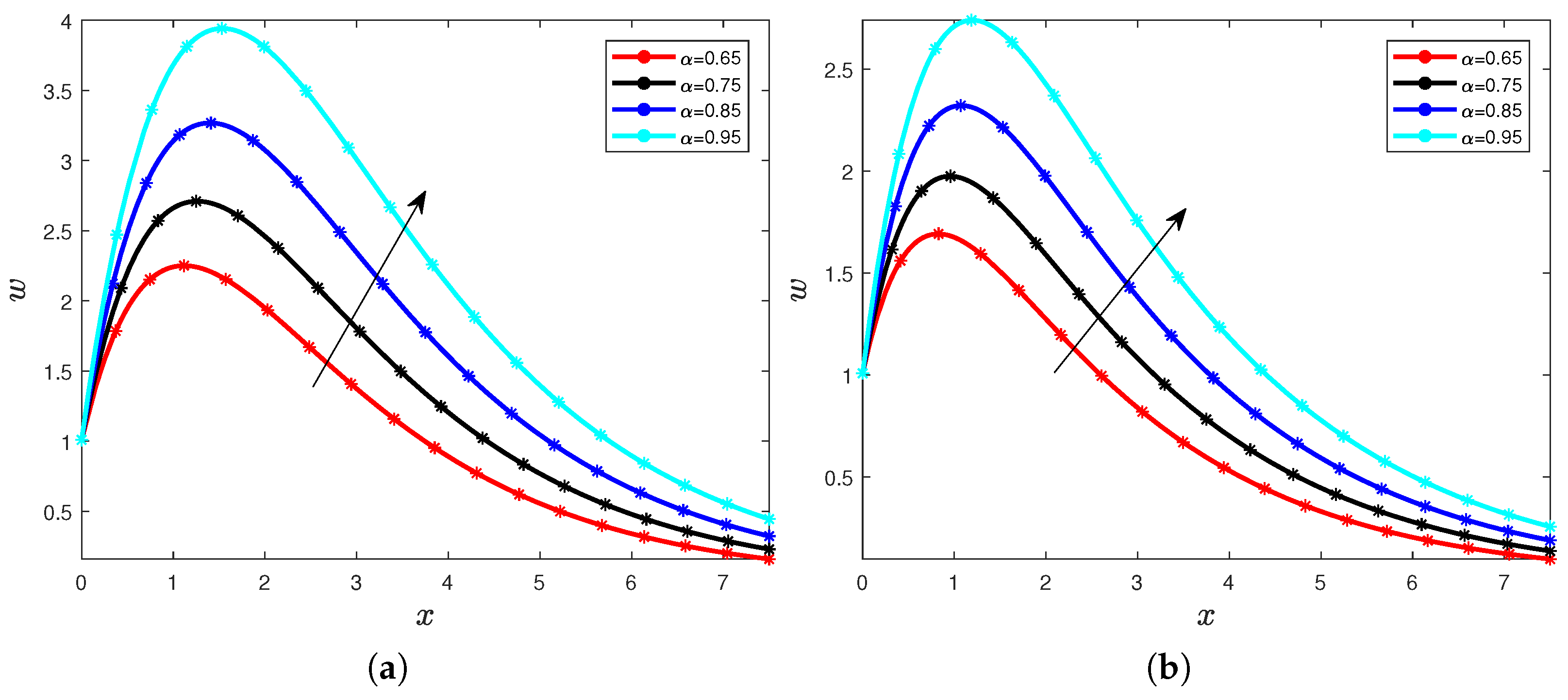
Figure 1. Velocity for different values of the order α with Pr = 5 (a) and Pr = 10 (b).
Mathematics 10 01125 g001
Figure 2. Velocity for different values of the order α with Pr = 15 (a) and Pr = 20 (b).
Mathematics 10 01125 g002
Figure 3. Velocity for different values of the order α = 0.65 (a) and α = 0.75 (b).
Mathematics 10 01125 g003
Figure 4. Velocity for different values of the order α = 0.65 (a) and α = 0.75 (b).
Mathematics 10 01125 g004
Figure 5. Velocity for different values of the Casson parameter η = 0 (a) and η = 0.3 (b).
Mathematics 10 01125 g005
Figure 6. Velocity for different values of the Casson parameter η = 0.5 (a) and η = 1 (b).
Mathematics 10 01125 g006
Figure 7. Temperature for different values of the fractional order with P r = 10 (a) and P r = 15 (b).
Mathematics 10 01125 g007
Figure 8. Temperature for different values of the fractional order with P r = 10 (a) and P r = 15 (b).
Mathematics 10 01125 g008
Figure 9. Temperature for different values of the Prandtl number with α = 0.65 (a) and α = 0.75 (b).
Mathematics 10 01125 g009
Figure 10. Temperature for different values of the Prandtl number with α = 0.85 (a) and α = 0.95 (b).
Mathematics 10 01125 g010
Figure 11. Temperature for different values of the Prandtl number with α = 0.65 (a) and α = 0.75 (b).
Mathematics 10 01125 g011
Figure 12. Temperature for different values of the Prandtl number with α = 0.85 (a) and α = 0.95 (b).
Mathematics 10 01125 g012
Figure 13. Velocity with the order α = 0.85 and α = 1 with P r = 5 (a) P r = 10 (b).
Mathematics 10 01125 g013
Figure 14. Velocity with the order α = 0.85 and α = 1 with G r = 5 (a) G r = 10 (b).
Mathematics 10 01125 g014
Table 1. Parameter descriptions.
ParametersDescriptions
ρ density kg m 3
μ dynamic viscosity kg m 1 s 1
α 1 first normal stress module
gacceleration due to gravity m s 2
β volumetric coefficient of thermal expansion K 1
c p specific heat of the fluid at constant pressure J kg 1 K 1
κ thermal conductivity W m 1 K 1
ν Kinematics viscosity of the fluid m 2 s 1
Table 2. P r number values versus N u number values for the various values of time.
TimePrandtl NumberNusselt Number
0.1105.43022
0.1156.65063
0.1207.67948
0.1258.58592
0.4103.0126
0.4153.68967
0.4204.26046
0.4254.76334
0.7102.37493
0.7152.90868
0.7203.35865
0.7253.75509
Publisher’s Note: MDPI stays neutral with regard to jurisdictional claims in published maps and institutional affiliations.