Article

Numerical Modelling of Vibration Responses of Helical Gears under Progressive Tooth Wear for Condition Monitoring

1
Department of Vehicle Engineering, Taiyuan University of Technology, Taiyuan 030024, China
2
Centre for Efficiency and Performance Engineering, University of Huddersfield, Huddersfield HD1 3DH, UK
*
Author to whom correspondence should be addressed.
Mathematics 2021, 9(3), 213; https://doi.org/10.3390/math9030213
Submission received: 24 December 2020 / Revised: 17 January 2021 / Accepted: 18 January 2021 / Published: 21 January 2021

Abstract

:
Gear wear is a common fault that occurs in a gear transmission system that degrades the operating efficiency and may cause other catastrophic failures such as tooth breakage and fatigue. The progressive wear of a helical gear and its influences on vibration responses are rarely investigated due to the combined effects of the complicated lubrication state and the time-varying characteristic. To fill this gap, a numerical study was put forward to investigate the interactions between gear wear and dynamic response. In this study, an Archard’s wear model with elastohydradynamic lubrication (EHL) effect is adopted to simulate the helical gear wear, which is incorporated with an eight-degree of freedom dynamic model for understanding the gear dynamic at different wear degrees. The wear model shows that the gear wear mainly happens at the gear root due to the relative high slide-to-roll ratio. The dynamic modelling results demonstrate that the wear causes a reduction in time-varying gear mesh stiffness further leads to more vibration. Besides, the simulated vibration responses and experimental validation show that the wear cause increases in the amplitudes of the gear mesh frequency and its harmonics, which can reflect the evolution of progressive gear wear and can be used as monitoring features of gear wear.

1. Introduction

The helical gearbox is the most common apparatus used in various applications such as helicopters, automobiles, wind turbines and marine power trains for transmitting power and speed and altering the direction of motion. Normally, these applications work under high load conditions and variant lubrication states, and suffer from extreme environmental conditions. Thus, gears will inevitably get worn and even fail with some critical faults like tooth breakage and tooth plastic deformations. Gear tooth surface wear is a common early fault that takes place over a long period of service time. The gear wear can cause a deviation of tooth profile from its ideal profile, thus causing a reduction in gear mesh stiffness and further altering the vibration responses of a gear train. However, the effects of the progressive helical gear wear on the dynamic responses are not comprehensively investigated yet, which increases the difficulties in condition monitoring of gear wear.
In the past few decades, many numerical studies have been carried out to simulate the wear process in mechanical contact, among which the commonly used model is the Archard’s wear equation [1,2] proposed based on the theory of asperity contact. For instance, Stanković et al. [3] tried to experimentally determine the Archard’s wear coefficient for sliding bearings. Osman [4] studied the dynamic influences of tooth wear on gear trains. Moreover, there are some other literatures [5,6,7] addressing the modelling of tooth wear, but the wear depth was usually derived from the dry-contact Archard’s wear model, which did not take the lubrication effect into consideration. In fact, for most industrial applications, gears work under lubrication in which the mating surfaces are separated by a thin lubricant film to avoid direct metal-to-metal contact. Therefore, taking into account the lubrication effect is critical necessary to reflect the real wear state. Johnson [8] first proposed the concept of the load sharing in mixed elastohydradynamic lubrication (EHL), which illustrates that the load between the mating surfaces is shared by the lubricant film and asperity contact. Since then, researchers have paid particular attention to the wear occurred in lubrication state. Masjedi [9,10] introduced a method to rapidly calculate the friction coefficient and wear rate in mixed EHL regime taking into account the temperature rise, central film thickness and asperity load ratio. Afterwards, the method was employed on the wear prediction of spur gears by the authors. Based on Masjedi’s study, Wang et al. [11] utilised the method proposed to determine the wear depth for helical gear contact in mixed EHL. Although some studies have considered the wear effects under lubrication state, most of them are focused on the spur gears. Nevertheless, the time-varying characteristic caused by the helical angle brings many difficulties to the numerical simulation. Therefore, the wear simulation of helical gears under lubrication has not been fully studied.
Dynamic model analysis is a very popular method that can study the gear dynamic characteristics from the theoretical point of view. Ding [12] combined a dynamic model with a tooth wear model to investigate the interactions between tooth wear and dynamic behaviours. The results demonstrate that there is a two-way interaction between wear and dynamic behaviours. Liu [7] put forward a prediction model to study the nonlinear correlations between gear wear and dynamic responses of a spur gear set. Ma et al. [13] proposed an improved model for determining the gear mesh stiffness with tip relief, which gives good guidance to study the gear dynamics with wear. These relevant studies demonstrated that the surface wear will alter the gear involute profile, and thus cause a reduction in gear mesh stiffness, changes in contact load and also variation in the transmission errors. Finally, it leads to abnormal vibration and dynamic behaviours. The wear can cause many random and interval variables that increases the uncertainties in dynamics as well [14]. However, at the incipient stage, the wear-related signals are quite weak, which brings many difficulties to monitor the wear state of gears. Researchers are dedicated to realizing the condition monitoring of gear wear in recent years. Some promising works have been carried out to fulfil this goal. Hu [15] developed a state vector extracted from the Time Synchronous Averaging (TSA) vibration signal to evaluate the effect of wear on gear performance. The indicator consists of the sideband information which can reflect the deterioration in gearbox vibration caused by wear. Brethee [16] studied helical gear wear both numerically and experimentally, and the results show that the gear meshing frequency shows a distinguishable increasing trend with the increase in wear severity. Loutas [17] combined the vibration analysis, acoustic emission analysis and oil debris analysis to conduct condition monitoring of rotating machinery. The integration of these three methods increases the diagnostic capacity and reliability. Zhang [18] investigated the modulation signal of gear vibration and used a sideband estimator to monitor the wear process, and a promising result had been demonstrated in this work. Based on the research work presented above, vibration analysis is capable of monitoring the gear wear process, and the meshing frequency and its sideband information contain valuable information for fault diagnosis.
Aiming at the issues addressed above, this study investigates the dynamic responses of helical gear induced by the progressive gear tooth wear through an eight-degree of freedom dynamic model incorporated with an Archard’s wear model under mixed EHL regime. Moreover, the changes in gear mesh stiffness induced by gear wear are comprehensively studied. The simulated vibration responses are validated by an experimental study, which is very beneficial for the condition monitoring of progressive gear wear. This paper is organised as follows. Section 2 introduces the wear depth modelling process based on the Archard’s wear model with EHL effect. Section 3 presents the modelling process of dynamic responses of a helical gear set through an eight-degree of freedom dynamic model, in which the changes in gear mesh stiffness caused by tooth wear were investigated in detail. Section 4 illustrates the simulated dynamic responses at different running hours, which are further verified by an experimental study. Last, several conclusions are drawn in Section 5.

2. Gear Tooth Wear Modelling

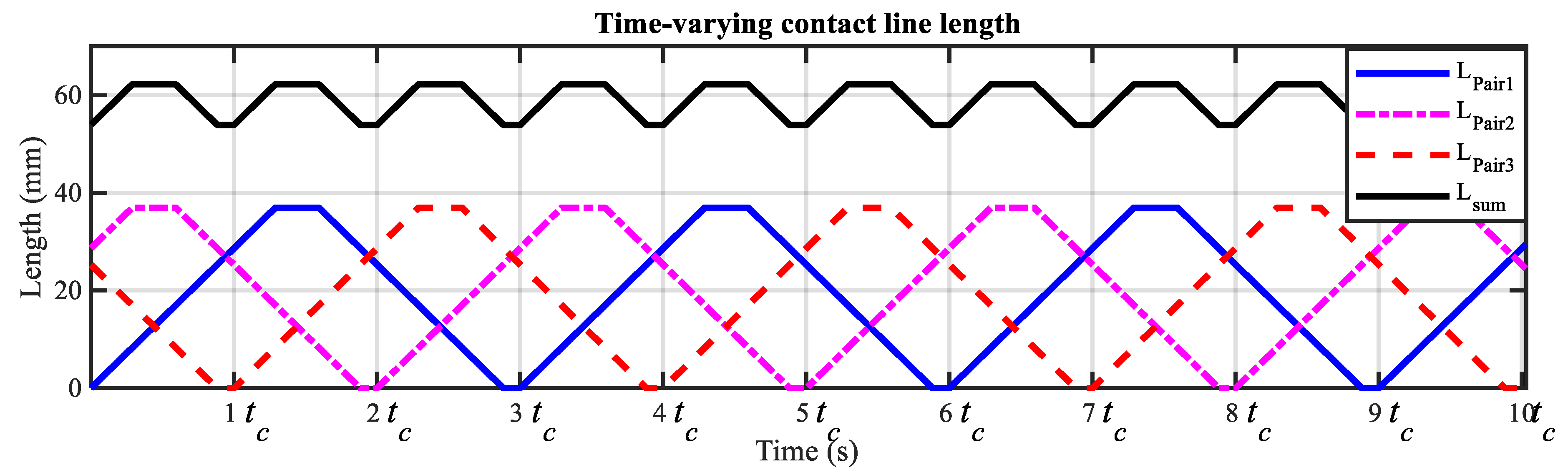
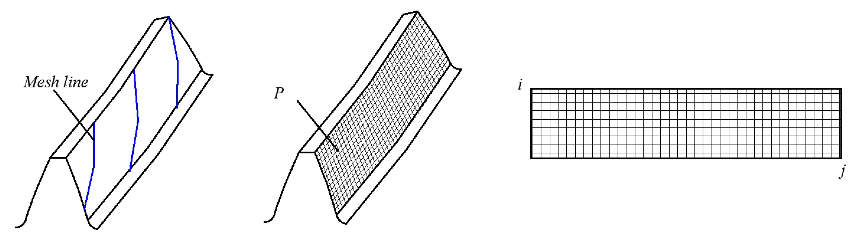
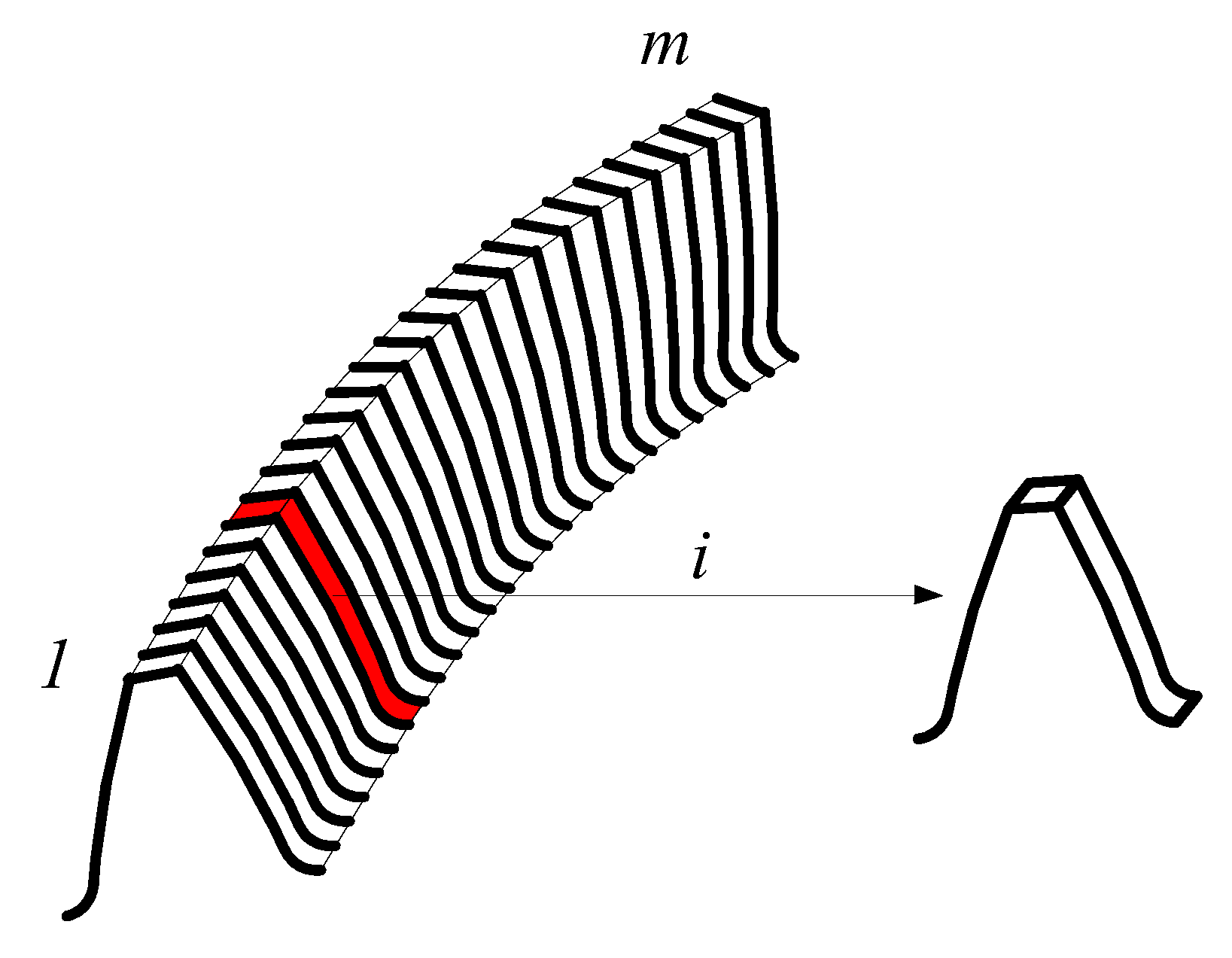
2.1. Mesh Characteristics of Helical Gear

For an ideally mounted spur gear pair, when the gear tooth enters the mesh area, the contact line length of the mesh tooth pair is constant and equal to the tooth width. However, for helical gears, the contact line length of one mesh tooth pair is time-varying due to the existence of the helical angle. As shown in Figure 1, the time-varying contact line length of one mesh tooth pair of a helical gear set can be classified into two categories:
L i ( t ) = { L C D csc β γ ( t ) ,   ε α ε β b sec β γ ( t ) ,   ε α > ε β
where b is the tooth width, β is the helical angle and γ ( t ) is the periodic piecewise linear function which can be expressed as
γ ( t ) = {   t ε o ,   0 t ε o   1 ,   ε o t ε t 1 ( t ε t ) ε o ,   ε t t ε   0 ,   ε t n
where ε 0 is the overlap ratio and ε t is the transverse contact ratio, the total contact ratio ε = ε 0 + ε t . t = m o d ( t , n t c ) / t c .   n = c e i l ( ε ) , t c is the time duration of the normal pitch which can be calculated as t c = P b ω g r b g . ω g , r b g represent the angular velocity and the radius of the base circle of the gear respectively. P b is the base pitch.
Figure 2 depicts the time-varying contact line length of a pair of helical gears which was selected from the experimental study, for detailed specification see Section 4.4.1. It can be observed that when tooth pair 1 starts to enter the meshing area, its contact line length increases gradually, then remains constant for a period of time and decreases gradually until the mesh point exits the meshing area. As the gear rotates, the gear teeth enter the meshing area in a certain sequence, and the total contact line length can be determined by adding the contact line lengths of all the meshing tooth pairs in the contact region simultaneously.
Compared with spur gears, due to the helical angle, the gear mesh impact generated due to the mesh-in and mesh-out actions can be effectively reduced. However, also due to this time-varying characteristic of the helical gear, the numerical modelling of progressive gear wear is very challenging because there are many time-varying variables, and the wear is also unevenly distributed on the tooth surface due to the loading sharing characteristic. Therefore, to overcome the difficulty induced by the time-varying characteristic, the tooth surface of the helical gear was divided into a grid with i × j segments as shown in Figure 3. By determining the wear depth of each local meshing point P, the wear depth of the helical gear can be simulated. The following section will introduce a wear model to estimate the wear of helical gear in the mixed EHL condition.

2.2. Modelling of Gear Wear under Mixed EHL Regime

In order to make the wear modelling comparable with the experimental validation, the same gear parameter as the gearbox 2 from a real test study was selected for modelling. For detailed parameters, please refer to Section 5. The simulated gearbox comprises of two stages: the first stage works at low speed and the second stage works at high speed. First, the lubrication state of the two stages needs to be determined in order to accurately simulating the wear depth. According to the equation proposed by Dowson and Higginson [19], the lubrication regime can be distinguished by the film thickness ratio which equals to the thickness of the minimum oil film h m i n divided by the composite surface roughness R e :
λ = h m i n R e = 1.6 α p v 0.6 ( η 0 u r ) 0.7 ( E ) 0.03 ρ 0.43 w 0.13 R e
where the definitions of the variables in Equation (3) can be found in Table 1, and u r ,   ρ ,   w can be calculated using the gear specification illustrated in Table 2 and the corresponding working conditions for each stage, respectively.
It can be noticed in Figure 4 that, for the low-speed stage, λ is around 1.48, and for the high-speed stage, λ is around 5. According to the Stribeck curve [20], the first stage is working in mixed EHL regime and the second stage is working in full EHL regime. This implies that the first stage is more prone to wear due to the asperity contact in the mixed EHL regime. Thus, the following content will introduce a wear model in mixed EHL regime to determine the wear depth.
According to the publications produced by Archard [1], the traditional Archard’s wear equation which describes the wear of dry contact can be written as
V = K F n H S
where V is the volume of wear. S is the relative sliding distance between the two meshing points. K is the non-dimensional wear index. F n is the normal force applied on the contact region. H is the hardness of material. Dividing both sides of Equation (4) by time t yields
V t = K F n H u s
where V t stands for the wear volume per unit time and u s is the sliding velocity between two mating surfaces. However, the mating gears usually work in the mixed EHL regime, in which the load between the mating surfaces is shared by the asperities and the lubricating film simultaneously. According to research by Masjedi and Khonsari [21], the wear volume per unit time in the mixed EHL regime can be rewritten as
V lub = K Ψ ( L a 100 ) F n H u s
where V lub is the wear volume per unit of time in the mixed lubrication, and L a and ψ are the asperity load ratio of the two contact surfaces and the fractional film defect, respectively, which can be expressed as
Ψ = 1 exp [ X u s t 0 exp ( E a R g T s ) ]
L a = 0.005 W 0.408 U 0.088 G 0.103                                                                                                                                                           × ln ( 1 + 4470 σ ¯ 6.015 V 1.168 W 0.485 U 3.741 G 2.898 )
where Χ , t 0 E a are parameters relating to lubrication which can be determined by experiments. R a is the molar gas constant and T s is the contact temperature. The parameters of W ,   U ,   G ,   V and σ ¯ are functions of the dimensionless load, speed, modulus, surface hardness and surface roughness, respectively, the expression of which can be found in [21].
Dividing both sides of Equation (6) by u s yields
V lub u s = K Ψ ( L a 100 ) F n H
Noticed that   V lub = A h and p = F n / A ( A is the contact area, h is the wear depth per unit of time, p is the average pressure value of all points in a local contact area), Equation (9) can be transformed to
h u s = K Ψ ( L a 100 ) p H
Therefore, the wear depth h i j of each local contact point P i j on the gear surface is
h i j = 0 S k Ψ i j ( L a 100 ) p i j d S
where k is the wear coefficient and can be written as k = K / H . According to Equation (11), the wear depth h i j at point i j on the gear tooth surface in mixed EHL is determined by the contact pressure p i j , the fractional film defect ψ i j and the sliding distance S .
To determine the contact pressure, the contact between the two mating teeth was regarded as the contact of two cylinders with parallel axes. As stated by the Hertzian contact theory, the half width of the contact area is
a h = 4 F t ρ π b E
where F t is the tangential force, and ρ and E can be found in Table 1.
Therefore, the contact pressure between the mating point is
p = 2 F t π a h b
Figure 5 shows the changing process of a pair of mating points of the gear and pinion in the contact area, respectively. As the two contact points have different peripheral velocities, the corresponding sliding distances of the gear and pinion can be, respectively, obtained by the following formulae.
S p = 2 a h u p u g u p
S g = 2 a h u g u p u g
where the subscript g, p stands for the pinion and gear respectively. u g and u p represent the peripheral velocities of the two mating points on the gears that can be estimated by
u g = ω g ( d g 2 sin α + y )
u p = ω p ( d p 2 sin α y )
where ω g , ω p denotes the rotational velocity. d g ,   d p denotes the gear pitch diameter. α represents the gear pressure angle. y represents the distance between the pitch point and the mating point.
As stated above, the contact pressure and the relative sliding distance of the mating point can be estimated by Equations (13)–(15), then the wear depth of the mating gears can be obtained by substituting them into Equation (11). The accumulated gear tooth wear after n revolutions can be estimated as
h i j , ( n ) = h i j , ( n 1 ) + 0 S k ψ i j ( L a 100 ) p i j d S i j
where h i j , ( n ) stands for the wear depth at the meshing point P i j on the tooth surface after n revolution, h i j , ( n 1 ) stands for the wear depth after n 1 revolution, and p i j stands for the corresponding pressure at meshing point P i j .
According to the wear model, a simulation of helical gear wear was carried out based on the parameters and working conditions of the first stage of the gearbox in the laboratory as depicted in Figure 15, the detailed parameters for the simulation can be found in Table 2. Figure 6a presents the wear depth simulated in the Archard’s wear model in EHL regime. In the direction of the line of action (LOA), when the meshing point moves from the tooth root to the tooth pitch, the wear depth decreases gradually, when it moves from the tooth pitch to the tooth tip, the wear depth increases gradually. Besides, due to the relative high sliding-to-roll ratio, the maximum wear took place close to the tooth root. In the direction of the tooth width, due to changes in the load sharing ratio and meshing tooth pairs, the wear depth shows uneven distribution on the tooth flank. Figure 6b shows the wear depth derived from the dry contact Archard’s wear model; the magnitude of the wear depth is much greater than that derived from the Archard’s wear model in EHL regime. This is because, in the absence of lubricant, the mating surfaces are in direct contact, which will generate greater friction and thus accelerate the wear process. However, in the mixed EHL regime, the load between the mating surfaces is shared by the lubricant film and the asperities, which can effectively reduce the direct asperity contact and significantly reduce the wear rate.

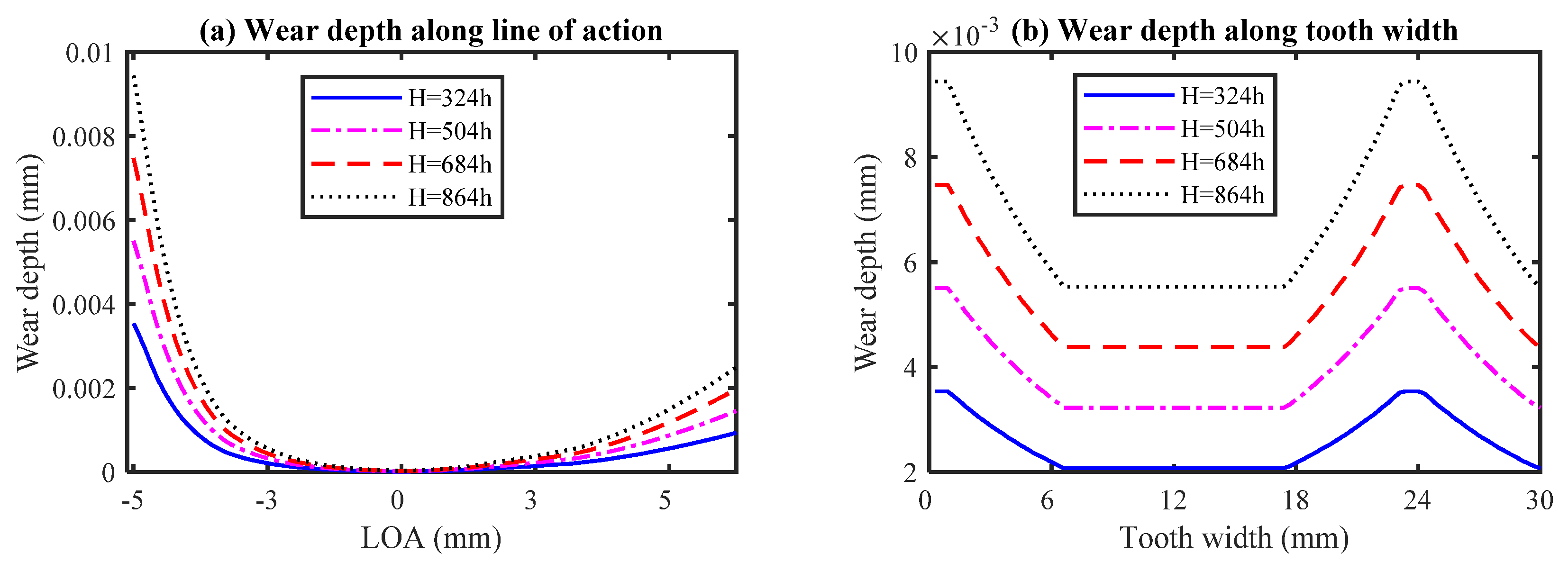
2.3. Wear Depth after Different Running Hours

To study the changes in wear with operating hours, four different times were selected with an interval of 180 h according to the experimental study in Section 4.4.2. Figure 7 shows the maximum tooth wear depth under different running hours. It can be observed that as time passes, the accumulated wear depth increases gradually. In the direction of LOA, the maximum wear depth is around 10 µm, which occurred on the tooth root due to the high relative sliding-to-roll ratio. In the direction of tooth width, the wear distributes the same as the sharing load allocated on the tooth surface. It implies that the high load results in more wear on the gear. According to the wear depth obtained, the following section will introduce a dynamic model to study the influence of the wear on the gear dynamic behaviour.

3. Dynamic Modelling of Helical Gear

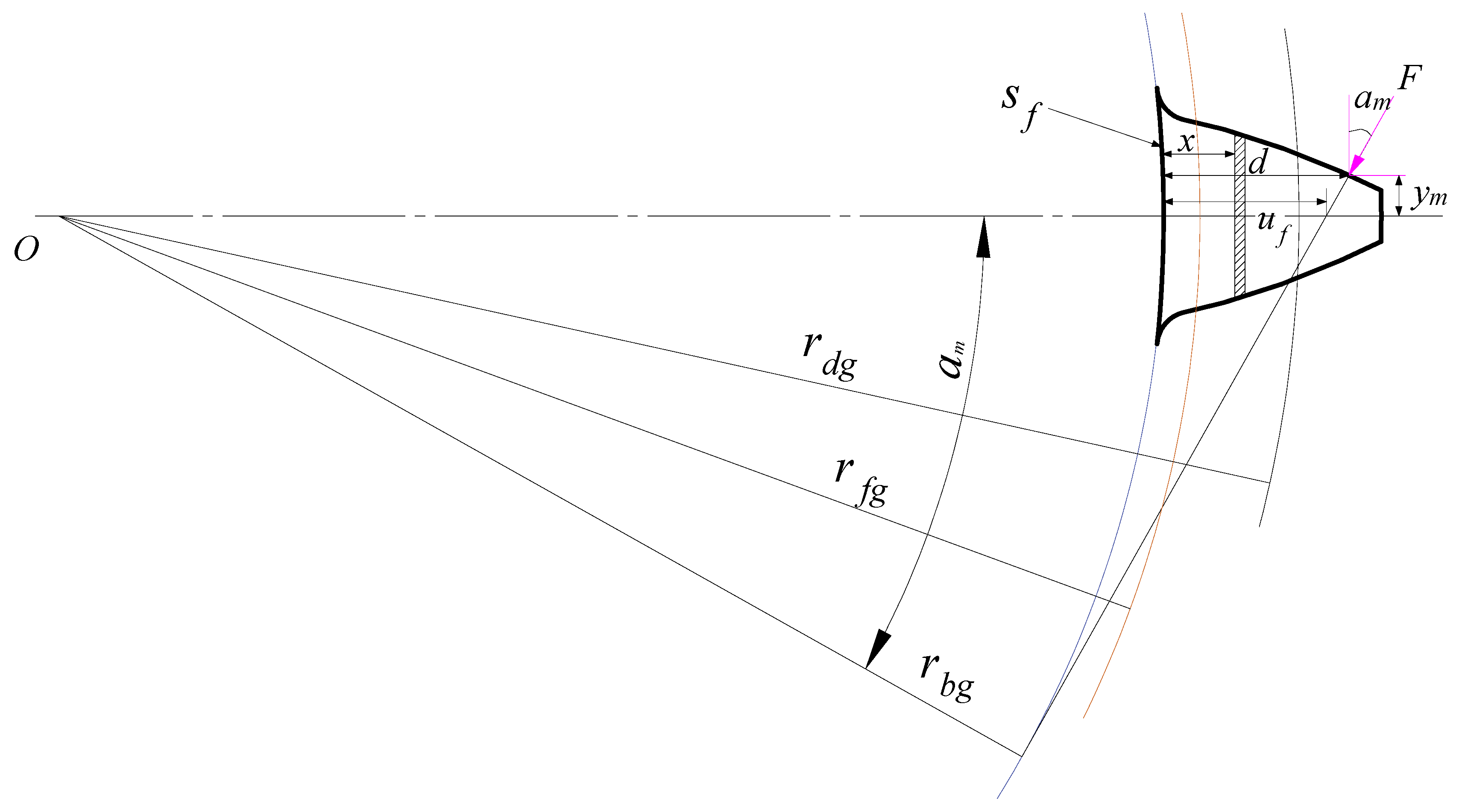
3.1. Potential Energy Method for TVMS Calculation

The potential energy method is a well-accepted method for calculating gear mesh stiffness. The method treats the gear as a nonuniform cantilever beam as shown in Figure 8. According to the work in [22], the time-varying mesh stiffness (TVMS) of a spur gear pair includes the Hertzian mesh stiffness k h , bending mesh stiffness k b , shear mesh stiffness k s , axial compressive stiffness k a and fillet-foundation stiffness k f , which can be determined by
U h = F 2 2 k h ,   where   k h = π E b 4 ( 1 ν 2 )
U b = F 2 2 k b = 0 d [ F b ( d x ) F a y m ] 2 2 E I x d x
U s = F 2 2 k s = 0 d 1.2 F b 2 2 G A x d x
U a = F 2 2 k a = 0 d F a 2 2 E A x d x
U f = F k f = F cos 2 α m E b { L * ( μ f S f ) 2 + M * ( μ f S f ) + P * ( 1 + Q * tan 2 α m ) }
where F stands for the contact force. F a ,   F b are the radial and tangential forces. α m is the operating pressure angle. G is the shear modulus. S n is the shear factor.   u f ,   S f ,   h ,   d and x are depicted in Figure 8. I x and A x are the inertia moment and area of the shaded part, respectively, as illustrated in the figure, the calculation of which can refer to the publication [23]. The coefficients L * ,   M * ,   P * ,   Q * can be obtained by the polynomial function proposed by Sainsot [24].

3.2. TVMS Calculation of Helical Gear with Tooth Wear

For helical gear, the gear tooth can be regarded as a combination of multiple spur gears with different angles as shown in Figure 9, thus the total TVMS can be determined by summing up the stiffnesses of all the spur gear slices at the meshing area at every time instant.
When the wear occurred on the gear tooth surface, the gear tooth profile will be altered as shown in Figure 10, thus the tooth thickness of each spur gear slice will be reduced. Correspondingly, the coordinate of the meshing point will be changed as well. As a result, the gear mesh stiffness will be affected. In order to more accurately assess the gear mesh stiffness of worn gears, the involute profile of each spur gear slice was updated with its corresponding wear depth:
{ x p = r b g ( sin α α cos α ) h p , n sin α m y p = r b g ( cos α + α sin α ) h p , n cos α m
where α is the transverse pressure angle at pitch point. The mesh stiffness k i t of each spur gear slice at time t can be estimated by the following equation:
k i t = 1 k h i t + k b g i t + k b p i t + k s g i t + k s p i t + k a g i t + k a p i t + k f g i t + k f p i t
The total TVMS k m t at the time instant t equals to the summation of the stiffnesses of all the spur gear slices at the meshing region:
k m t = i = 1 n k i t
The damping coefficient of the meshing gears can be calculated as
c m t = 2 ξ k m t m e
where m e stands for the equivalent mass of the gears and ξ denotes the viscous damping ratio.

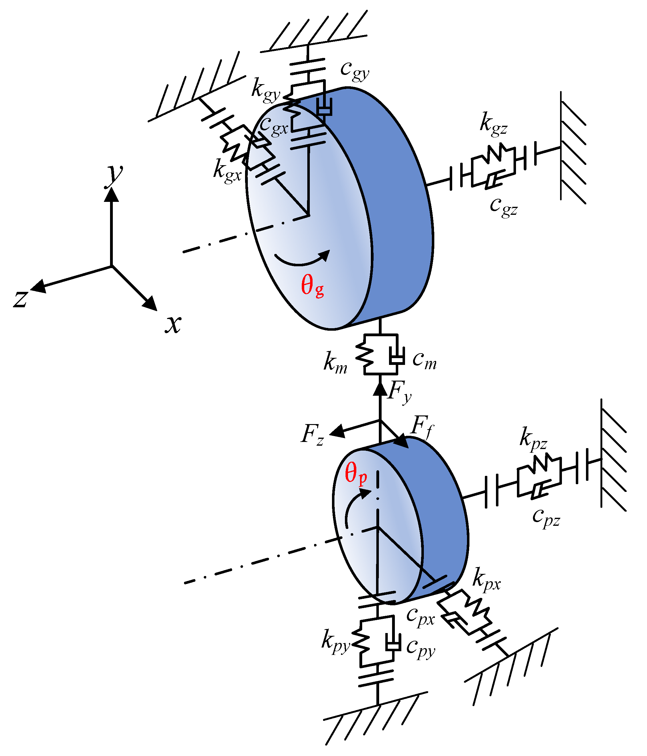
3.3. An Eight-Degree of Freedom Dynamic Model

To study the dynamic responses of the helical gear caused by progressive tooth wear, a dynamic model which has eight degrees of freedom was put forward, as demonstrated in Figure 11. The gearbox used in the experimental study was a two-stage gearbox. However, the study of lubrication state illustrates that the low-speed stage is more prone wearing due to the poor lubrication state, so the dynamic model will only focus on the low-speed stage for simplifying the computation and eliminating the irrelevant factors. In this model, the shaft, gear and pinion are considered rigid, and the ball bearings were treated as linear spring–damping unit. In total, this model includes two torsional motions and six translational motions along the direction of the line of action (LOA), radial direction and axial direction. The governing equations can be written as
{ m g y ¨ g + c g y y ˙ g + k g y y g = F y m g z ¨ g + c g z z ˙ g + k g z z g = F z m g x ¨ g + c g x x ˙ g + k g x x g = F f I g θ ¨ g = T d F y r b g + F f ( r b g tan α m H ) m p y ¨ p + c p y y ˙ p + k p y y p = F y m p z ¨ p + c p z z ˙ p + k p z z p = F z m p x ¨ p + c p x x ˙ p + k p x x p = F f I p θ ¨ p = T L + F y r b p F f ( r b p tan α m + H )
where Ii represents the inertia moment. mi stands for the mass of the gear. θ i represents the angle of rotation. x i ,   y i ,   z i denote the translational displacement in x, y, z directions, respectively. ci and ki, respectively, denote the damping constant and stiffness constant of the bearing. Td, TL are the loads applied on the driving gear and driven pinion. rbg, rbp are the radius of the base circle of gear and pinion. H is the distance from the mesh point to the pitch point. Fm, Ff are the dynamic meshing force and friction force that can be estimated by
{ F y = k m t cos β ( y ˜ g y ˜ p ) + c m t sin β ( y ˜ ˙ g y ˜ ˙ p ) F z = k m t sin β ( z ˜ g z ˜ p ) + c m t cos β ( z ˜ ˙ g z ˜ ˙ p ) F f = μ ( t ) F y 2 + F z 2
where k m t , c m t can be derived from the Equations (26) and (27). μ ( t ) is the time-varying friction coefficient found in [25]. y ˜ ˙ g , y ˜ ˙ p , z ˜ ˙ g , z ˜ ˙ p are the derivatives of y ˜ g , y ˜ p , z ˜ g , z ˜ p , which can be calculated as
{ y ˜ g = y g + r b g θ g ,   y ˜ p = y p r b p θ p z ˜ g = z g + y ˜ g tan β ,   z ˜ p = z p y ˜ p tan β

4. Modelling Results and Experimental Study

4.1. Changes in Gear Meshing Stiffness and Meshing Force

As aforementioned, gear mesh stiffness can be derived using the potential energy method in which the tooth thickness plays an important role to determine the stiffness. Figure 12a demonstrates the total time-varying mesh stiffness which fluctuates periodically due to the changes in total meshing tooth pairs. Besides, note that the mesh stiffness shows a decreasing trend with the growth of the wear depth, which mainly occurs due to the reduction in tooth thickness. Figure 12b–d presents the dynamic meshing force along the y, z, x directions. As can be observed in the zoom-in figures, the meshing force increases gradually with the increase in running hours. This is because the gear wear reduces the mesh stiffness, causing more deformation in contact area, which then leads to an increase in meshing force.

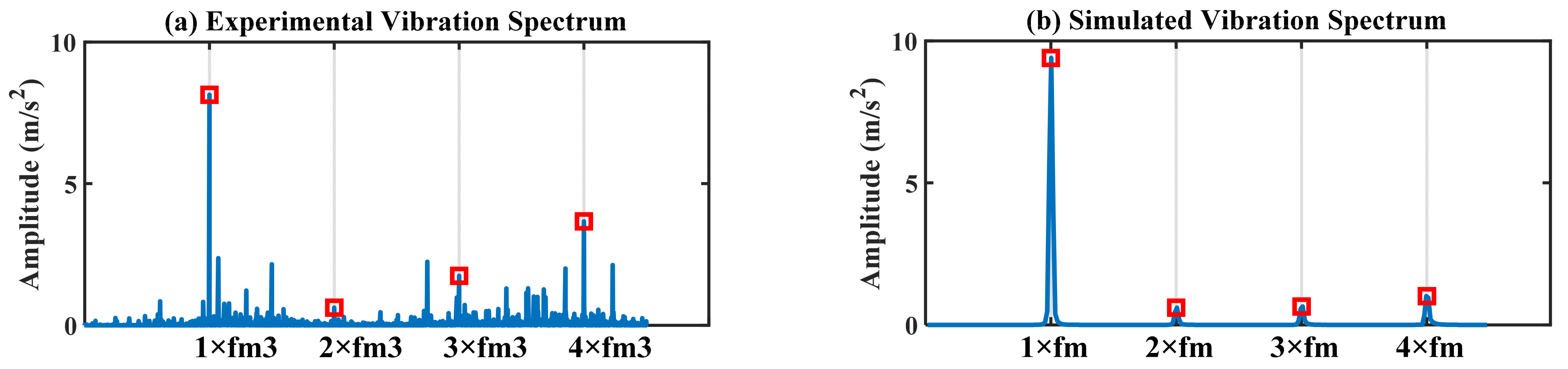
4.2. Raw Spectrum Comparison between Simulated Vibration and Experimental Vibration

The simulated vibration responses are in three dimensions, which will finally transmit to the body of the gearbox through the shaft and bearing eventually, so the vibration of the gearbox body was the superposition of the vibration in these three directions. Hereby, the root mean square (RMS) value was adopted to evaluate the integral vibration fint of the gearbox body:
f int = f xv 2 + f yv 2 + f zv 2 3
where fxv, fyv, fzv stand for the vibration signals in x, y, z directions in the frequency domain. fint stands for the integral vibration in the frequency domain. Figure 13a exhibits the spectrum of the vibration signal acquired experimentally. The test rig description is detailed in Section 4.4.1. As shown in the figure, the gear meshing frequency and its corresponding harmonics can be clearly observed. Figure 13b shows the simulated vibration spectrum derived from the dynamic model. The two spectra have similar vibration responses that the fundamental meshing frequency is dominated in both of the two figures. Moreover, the harmonics show relatively low amplitudes but an increasing trend with the increase of harmonic order. For the experimental vibration spectrum, there are some other frequency components as it includes the background noise from the bearings, motor and the second stage of meshing gear pair, etc.

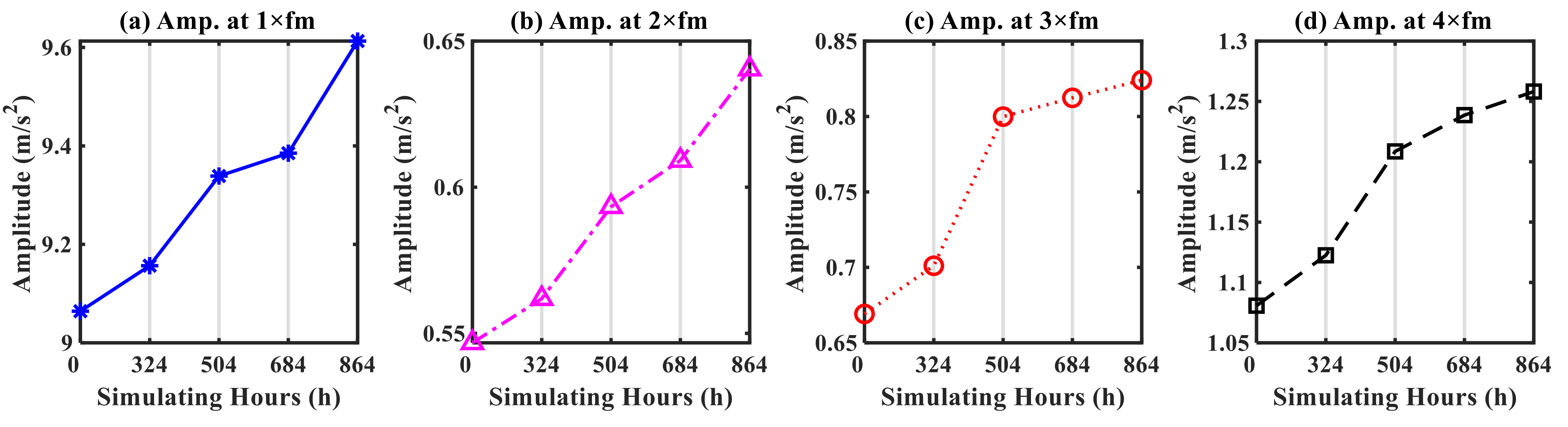
4.3. Simulation Results under Different Operating Hours

To get a distinguishable indication of the changes in the vibrations, the amplitudes of the first four harmonics of the meshing frequency were extracted from the spectrum of the integral vibration under the different operating hours. The variation in the amplitude was depicted in Figure 14. As the figure demonstrates, the amplitudes of the meshing frequency and its corresponding harmonics show an increasing trend with the increase of operating time. This is because the wear depth accumulated with the increase of operating time, then leads to the increase in the meshing force in both x, y, z dimensions as previously mentioned, further cause the increase in the gear vibrations. The incremental trend can be an indicator for reflecting the wear evolution process.

4.4. Experimental Results under Different Operating Hours

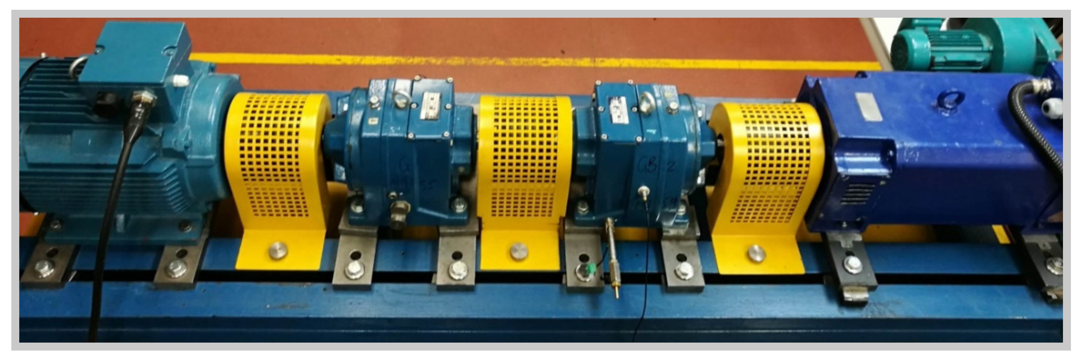
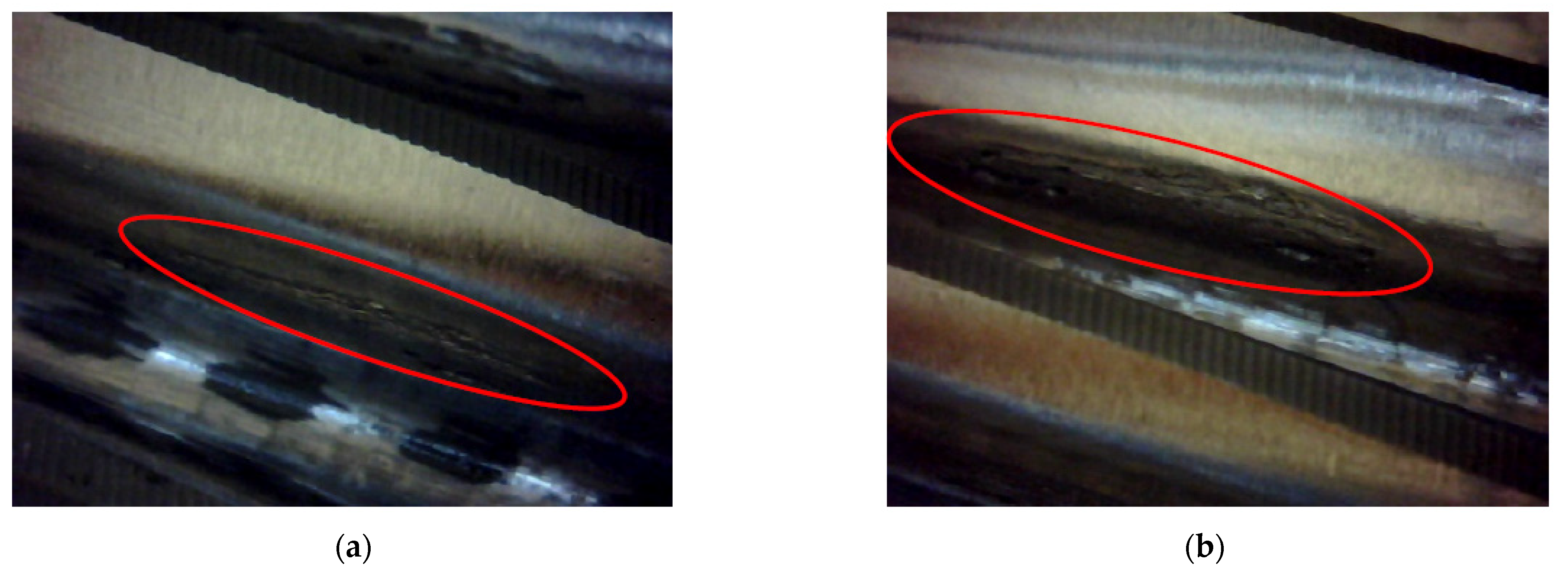
4.4.1. Description of Experimental Bench

To simulate the process of the progressive wear more precisely and naturally in the laboratory environments, a run-to-fatigue test that lasted more than 800 h was performed on a helical gearbox test rig under variant working conditions, which makes the simulation close to the scenarios of many real-world gearbox applications like wind turbines and helicopters. Figure 15 details the basic structure of the test rig. Two industrial gearboxes were installed back-to-back, which were, respectively, connected with an AC drive motor (15 kW) and a DC load generator (17.5 kW). The geometric parameters of the two helical gearboxes used in this study are shown in Figure 15. For the first stage of gearbox1 (GB1), the gear acts as a driving gear while the pinion is driven. The operating conditions were manipulated by a Variable Speed Drive and Load Controller (VSD). Two accelerometers were mounted on the block surfaces of GB1 and GB2 respectively for collecting the vibration signals. A sixteen-channel data acquisition system was used to collect the vibration, acoustic, oil temperature and encoder signals in 30 s under each working condition.
The test was run for 868 h and then stopped due to the noticeably high peak of GB2 vibration that occurred. During this process, the gearbox was never dissembled to ensure the installation state of the gears and the rig is the same throughout the whole test. After opening the gearbox, the wear was observed to happen in GB2 at the low-speed stage. As presented in Figure 16, the visible wear was generated naturally close to the gear tooth root due to the relative high sliding-to-roll ratio. This is in line with the theoretical study.

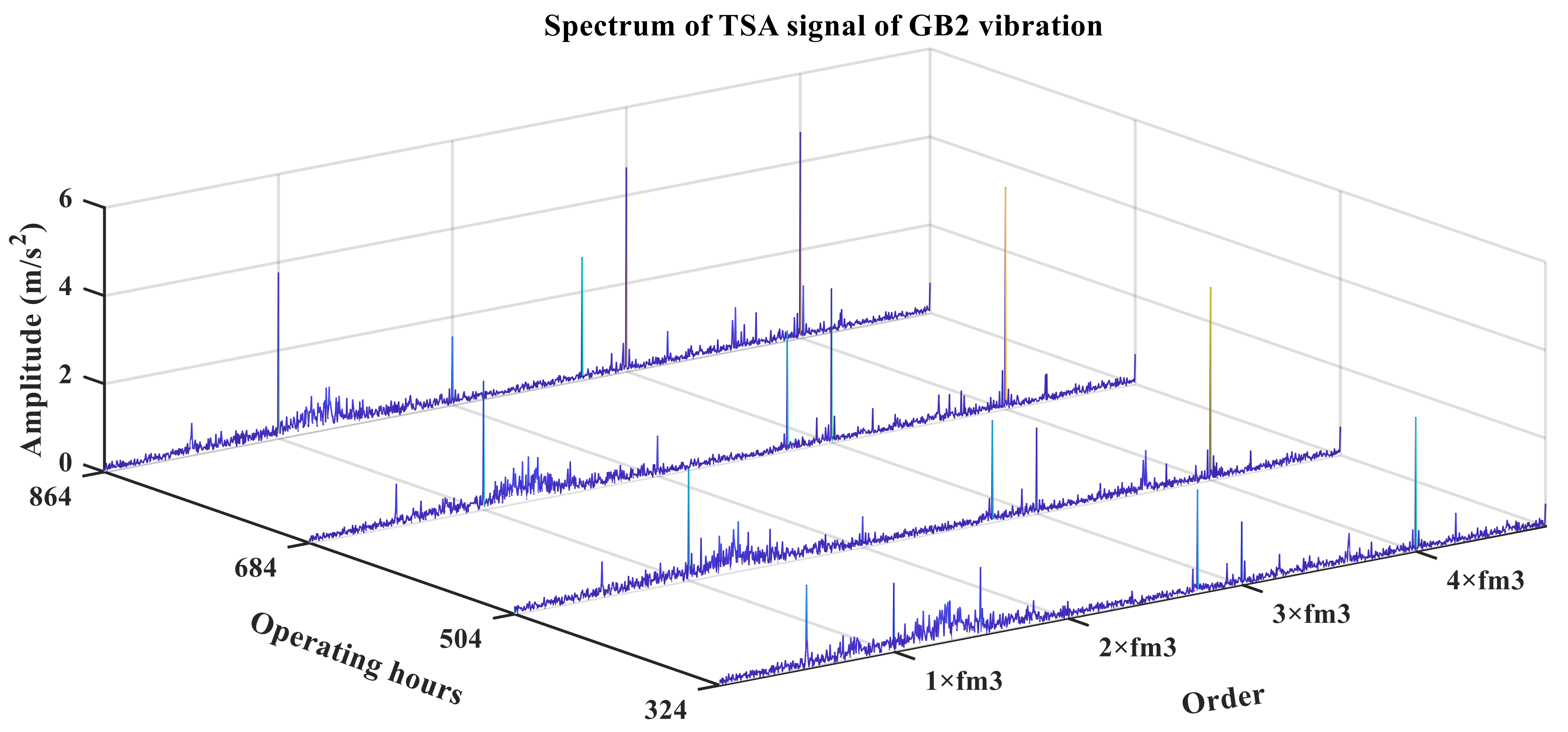
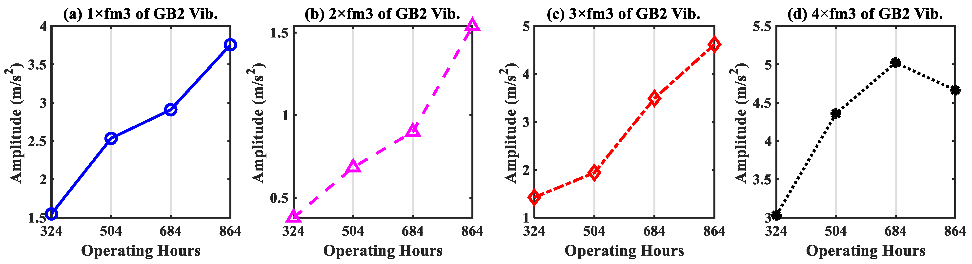
4.4.2. Feature Extracted from Experimental Vibration Spectrum

The data collected were divided into two sets: the first set is the data collected before 324 h, during which the gears were working at the break-in stage, which leads to more vibration and noise. However, as time passes, the gear tooth surfaces will be gradually ground and become smooth. The following stage is the progressive wear developing period under mixed EHL. In this period, the vibration and noise vary with the changes in surface topography of the mating tooth. With the development of the wear severity, the vibro-acoustic characteristics of GB2 deteriorate gradually. Therefore, to get more meaningful results, this study will focus on the data collected after 324 h at the operating condition of 70% speed (1039 rpm) and full load.
In order to indicate the development of wear, four sets of data with an equal time interval of 180 h were selected from the data for further analysis. Due to the superiority of time-synchronized averaging (TSA) in terms of noise reduction and signal enhancement, TSA was used to process the vibration signals for suppressing the background noise from bearing, motor and the other gear stage. Figure 17 demonstrates the TSA spectrum of the GB2 vibration signal under different operating hours. The high peaks in the frequency domain represent the meshing frequency fm3 and its corresponding harmonics. A clear increase in amplitude can be observed from the TSA spectrum, which reflects the deterioration of the gear dynamic due to wear.
Gear mesh impact is the main source of gearbox vibration and noise. Many gear faults can be identified by analysing the characteristic frequencies of a gearbox. Figure 18 depicts the evolution trends of the amplitudes of fm3 and its harmonics as shown in Figure 18a–d. A noticeable increase in the amplitudes at the frequency of   1 × f m 3 ,   2 × f m 3 ,   3 × f m 3 and   4 × f m 3 can be observed. However, the changes in f m 4 and its harmonics did not show any regular variation related to gear wear. First, the reason for the change between the two meshing frequencies f m 3   and f m 4 is that the wear mainly occurred at the low-speed stage because the relatively low slide-to-roll ratio cannot form a sufficient lubrication film, leading to inadequate lubrication and rapid wear. Moreover, the changes in the amplitudes of f m 3 and its harmonics demonstrate that the wear can significantly enlarge the gear mesh impacts due to the reduction in gear contact ratio and the contact pressure angle, thereby further dramatically deteriorates the gear dynamic characteristics. Through the experimental study, the evolution trends of f m 3 and its harmonics can effectively indicate the development of progressive gear wear. In addition, the experimental results have a good agreement with the numerical results indicating that the numerical model can give a reliable prediction of gear dynamics, and also providing a reliable theoretical basis for accurate fault diagnosis of progressive gear wear.

5. Conclusions

This study investigated the evolution process of the dynamic responses of a helical gear set induced by progressive gear wear both numerically and experimentally. First, the wear depth of the helical gear set was derived from an Archard’s wear model in mixed EHL condition. Then, the gear dynamic responses were derived from an eight-degree of freedom dynamic model which comprehensively considers the changes in gear meshing position due to wear. Besides, a gear run-to-fatigue test was conducted to validate the numerical results. The results obtained in this study can effectively reflect the progressive wear process of helical gears, and, at the same time, provide a theoretical basis for the condition monitoring of gear trains. Based on this research, the following conclusions can be drawn:
(1) The wear depth simulated from the Archard’s wear model with EHL effect is more reasonable than that derived from the traditional Archard’s wear model, as the lubricant can significantly reduce the friction effect between the mating surfaces. Besides, the wear mainly happens at the region close to the gear root due to the relative high sliding-to-roll ratio. The wear distribution along gear tooth width direction was also identified by load sharing.
(2) The simulation results show that the wear will cause a reduction in gear mesh stiffness and an increase in contact force, which further deteriorates the vibration responses. Correspondingly, the gear mesh frequency gives more valuable information to reflect gear wear process as the amplitudes of gear meshing frequency and its harmonics have increasing trends with the increase of wear depth.
(3) The experimental results show a good consistency with the numerical results. The wear significantly changes the vibration amplitudes of the meshing frequency and its harmonics. The increasing trends of the amplitudes can be effective indicators for condition monitoring the progressive wear in gear train. By employing appropriate advanced signal processing method, the gear tooth progressive wear can be identified using the changes in the amplitudes of the gear meshing frequency, which further can be used for diagnosing the gear wear.

Author Contributions

Supervision, T.W., F.G. and A.D.B.; Writing—original draft, X.S.; Writing—review and editing, R.Z. All authors have read and agreed to the published version of the manuscript.

Funding

This research was funded by the Natural Science Foundation of Shanxi Province, China (Grant number No. 201801D121181).

Institutional Review Board Statement

Not applicable.

Informed Consent Statement

Not applicable.

Data Availability Statement

Not applicable.

Acknowledgments

This study has achieved strong supports from the Gear Research Institute in Taiyuan University of Technology, the Centre for Efficiency and Performance Engineering in University of Huddersfield.

Conflicts of Interest

The authors declare no conflict of interest.

References

  1. Archard, J.F.; Hirst, W.; Allibone, T.E. The wear of metals under unlubricated conditions. Proc. R. Soc. Lond. Ser. A. Math. Phys. Sci. 1956, 236, 397–410. [Google Scholar] [CrossRef]
  2. Archard, J.F. Contact and Rubbing of Flat Surfaces. J. Appl. Phys. 1953, 24, 981–988. [Google Scholar] [CrossRef]
  3. Stanković, M.; Marinković, A.; Grbović, A.; Mišković, Ž.; Rosić, B.; Mitrović, R. Determination of Archard’s wear coefficient and wear simulation of sliding bearings. Ind. Lubr. Tribol. 2019, 71, 119–125. [Google Scholar] [CrossRef]
  4. Osman, T.; Velex, P. Static and dynamic simulations of mild abrasive wear in wide-faced solid spur and helical gears. Mech. Mach. Theory 2010, 45, 911–924. [Google Scholar] [CrossRef]
  5. Gu, Y.-K.; Li, W.-F.; Zhang, J.; Qiu, G.-Q. Effects of Wear, Backlash, and Bearing Clearance on Dynamic Characteristics of a Spur Gear System. IEEE Access 2019, 7, 117639–117651. [Google Scholar] [CrossRef]
  6. Kuang, J.H.; Lin, A.D. The Effect of Tooth Wear on the Vibration Spectrum of a Spur Gear Pair. J. Vib. Acoust. 2001, 123, 311. [Google Scholar] [CrossRef]
  7. Liu, X.; Yang, Y.; Zhang, J. Investigation on coupling effects between surface wear and dynamics in a spur gear system. Tribol. Int. 2016, 101, 383–394. [Google Scholar] [CrossRef]
  8. Johnson, K.L.; Greenwood, J.A.; Poon, S.Y. A simple theory of asperity contact in elastohydro-dynamic lubrication. Wear 1972, 19, 91–108. [Google Scholar] [CrossRef]
  9. Masjedi, M.; Khonsari, M.M. Theoretical and experimental investigation of traction coefficient in line-contact EHL of rough surfaces. Tribol. Int. 2014, 70, 179–189. [Google Scholar] [CrossRef]
  10. Masjedi, M.; Khonsari, M.M. An engineering approach for rapid evaluation of traction coefficient and wear in mixed EHL. Tribol. Int. 2015, 92, 184–190. [Google Scholar] [CrossRef]
  11. Wang, H.; Zhou, C.; Lei, Y.; Liu, Z. An adhesive wear model for helical gears in line-contact mixed elastohydrodynamic lubrication. Wear 2019, 426–427, 896–909. [Google Scholar] [CrossRef]
  12. Ding, H.; Kahraman, A. Interactions between nonlinear spur gear dynamics and surface wear. J. Sound Vib. 2007, 307, 662–679. [Google Scholar] [CrossRef]
  13. Ma, H.; Zeng, J.; Feng, R.; Pang, X.; Wen, B. An improved analytical method for mesh stiffness calculation of spur gears with tip relief. Mech. Mach. Theory 2016, 98, 64–80. [Google Scholar] [CrossRef]
  14. Fu, C.; Xu, Y.; Yang, Y.; Lu, K.; Gu, F.; Ball, A. Response analysis of an accelerating unbalanced rotating system with both random and interval variables. J. Sound Vib. 2020, 466, 115047. [Google Scholar] [CrossRef]
  15. Hu, C.; Smith, W.A.; Randall, R.B.; Peng, Z. Development of a gear vibration indicator and its application in gear wear monitoring. Mech. Syst. Signal Process. 2016, 76–77, 319–336. [Google Scholar] [CrossRef]
  16. Brethee, K.F.; Zhen, D.; Gu, F.; Ball, A.D. Helical gear wear monitoring: Modelling and experimental validation. Mech. Mach. Theory 2017, 117, 210–229. [Google Scholar] [CrossRef]
  17. Loutas, T.H.; Roulias, D.; Pauly, E.; Kostopoulos, V. The combined use of vibration, acoustic emission and oil debris on-line monitoring towards a more effective condition monitoring of rotating machinery. Mech. Syst. Signal Process. 2011, 25, 1339–1352. [Google Scholar] [CrossRef]
  18. Zhang, R.; Gu, X.; Gu, F.; Wang, T.; Ball, A.D. Gear Wear Process Monitoring Using a Sideband Estimator Based on Modulation Signal Bispectrum. Appl. Sci. 2017, 7, 274. [Google Scholar] [CrossRef]
  19. Dowson, D.; Higginson, G.R. Elasto-Hydrodynamic Lubrication: International Series on Materials Science and Technology; Elsevier: Amsterdam, The Netherlands, 2014; ISBN 9781483181899. [Google Scholar]
  20. Brandão, J.A.; Meheux, M.; Ville, F.; Seabra, J.H.O.; Castro, J. Comparative overview of five gear oils in mixed and boundary film lubrication. Tribol. Int. 2012, 47, 50–61. [Google Scholar] [CrossRef]
  21. Masjedi, M.; Khonsari, M.M. On the prediction of steady-state wear rate in spur gears. Wear 2015, 342–343, 234–243. [Google Scholar] [CrossRef]
  22. Wan, Z.; Cao, H.; Zi, Y.; He, W.; Chen, Y. Mesh stiffness calculation using an accumulated integral potential energy method and dynamic analysis of helical gears. Mech. Mach. Theory 2015, 92, 447–463. [Google Scholar] [CrossRef]
  23. Chaari, F.; Fakhfakh, T.; Haddar, M. Analytical modelling of spur gear tooth crack and influence on gearmesh stiffness. Eur. J. Mech. A/Solids 2009, 28, 461–468. [Google Scholar] [CrossRef]
  24. Sainsot, P.; Velex, P.; Duverger, O. Contribution of Gear Body to Tooth Deflections—A New Bidimensional Analytical Formula. J. Mech. Des. 2004, 126, 748–752. [Google Scholar] [CrossRef]
  25. Xu, H.; Kahraman, A.; Anderson, N.E.; Maddock, D.G. Prediction of Mechanical Efficiency of Parallel-Axis Gear Pairs. J. Mech. Des. 2007, 129, 58. [Google Scholar] [CrossRef]
Figure 1. Time-varying contact line length of one mesh tooth pair of helical gear. (a) case: ε α ε β ; (b) Contact line length when ε α ε β ; (c) case: ε α > ε β ; (d) Contact line length when ε α > ε β .
Mathematics 09 00213 g001
Figure 2. Contact line length of a helical gear pair.
Mathematics 09 00213 g002
Figure 3. Mesh grid on the gear tooth flank.
Mathematics 09 00213 g003
Figure 4. Film thickness ratio of the two stages in GB2. (LOA: line of action).
Mathematics 09 00213 g004
Figure 5. Relative sliding distance between the meshing points on the gear and pinion. (a) The starting point of engagement; (b) The ending position when the pinion exits the meshing area; (c) The ending position when the gear exits the meshing area.
Mathematics 09 00213 g005
Figure 6. Wear depth of the driving gear under. (a) Wear depth derived from Archard wear model with EHL; (b) Wear depth derived from conventional Archard wear model.
Mathematics 09 00213 g006
Figure 7. Maximum tooth wear depth under different running hours. (a) Wear depth along the line of action; (b) Wear depth along tooth width.
Mathematics 09 00213 g007
Figure 8. Modelling of nonuniform cantilever beam of spur gear.
Mathematics 09 00213 g008
Figure 9. Spur gear slices of helical gear.
Mathematics 09 00213 g009
Figure 10. Gear tooth contact point under different wear depth.
Mathematics 09 00213 g010
Figure 11. Schematic diagram of gear dynamic model.
Mathematics 09 00213 g011
Figure 12. Gear meshing excitations.
Mathematics 09 00213 g012
Figure 13. Comparison of experimental vibration spectrum and simulated vibration spectrum.
Mathematics 09 00213 g013
Figure 14. Amplitudes of the first four harmonics of the gear meshing frequency of simulated vibration. (a) Amplitudes of the first harmonic; (b) Amplitudes of the second harmonic; (c) Amplitudes of the third harmonic; (d) Amplitudes of the fourth harmonic.
Mathematics 09 00213 g014
Figure 15. Helical gearbox test rig diagram.
Mathematics 09 00213 g015
Figure 16. Worn gear of the low-speed stage in GB2. (a) Wear occurred on the pinion; (b) Wear occurred on the gear.
Mathematics 09 00213 g016
Figure 17. Spectrum of Time Synchronous Averaging (TSA) signal of GB2 vibration under different operating hours.
Mathematics 09 00213 g017
Figure 18. Amplitudes of f m 3 and its harmonics in the TSA spectrum. (a) Amplitude of the first harmonic 1 × fm3; (b) Amplitude of the second harmonic 2 × fm3; (c) Amplitude of the third harmonic 3 × fm3; (d) Amplitude of the fourth harmonic 4 × fm3.
Mathematics 09 00213 g018
Table 1. Values of the variables for calculating film thickness ratio.
hminMinimum film thickness, µmRecomposite surface roughness, 1.1 × 10⁻⁶ m
αpvPressure-viscosity factor, 2.03 × 10⁻⁸ m2/Nη0Lubricant viscosity, 0.2883 Pa·s
urRolling velocity, m/sEElastic modulus, 200 GPa
ρEquivalent radius, mE 2 / E = ( 1 ν 1 2 ) / E 1 + ( 1 ν 2 2 ) / E 2
wLoad per unit lengthνPoisson ratio, 0.28
kcThermal conductivity, W/m·KkWear coefficient, 1 × 10⁻¹⁶ m2/N
Table 2. Gearbox specifications.
Gearbox GB1GB2
Stage 1Stage 2Stage 1Stage 2
Teeth number, ZZr1/Zr2 = 49/55Zr3/Zr4 = 13/59Zi1/Zi2 = 59/13Zi3/Zi4 = 47/58
Helix angle, β (°)27131327
Centre distance, a (mm)74747474
Normal pressure angle, αn (°)20202020
Transverse pressure angle (°)22.2220.4820.4822.22
Gear tooth width, b (mm)25363625
Normal Module, mn (mm)1.25221.25
Transverse contact ratio, εt1.65141.59271.59271.6518
Overlap ratio, εo2.89021.28891.28892.8902
Young’s modulus, E (GPa)200200200200
Poisson ratio, ν0.280.280.280.28
Surface roughness, σ (µm)0.80.80.80.8
Vickers hardness, Hd (Pa)6.865 × 1096.865 × 1096.865 × 1096.865 × 109
Publisher’s Note: MDPI stays neutral with regard to jurisdictional claims in published maps and institutional affiliations.

