The Approximate Analytic Solution of the Time-Fractional Black-Scholes Equation with a European Option Based on the Katugampola Fractional Derivative

Abstract

In the finance market, it is well known that the price change of the underlying fractal transmission system can be modeled with the Black-Scholes equation. This article deals with finding the approximate analytic solutions for the time-fractional Black-Scholes equation with the fractional integral boundary condition for a European option pricing problem in the Katugampola fractional derivative sense. It is well known that the Katugampola fractional derivative generalizes both the Riemann–Liouville fractional derivative and the Hadamard fractional derivative. The technique used to find the approximate analytic solutions of the time-fractional Black-Scholes equation is the generalized Laplace homotopy perturbation method, the combination of the generalized Laplace transform and homotopy perturbation method. The approximate analytic solution for the problem is in the form of the generalized Mittag-Leffler function. This shows that the generalized Laplace homotopy perturbation method is one of the most effective methods to construct approximate analytic solutions of the fractional differential equations. Finally, the approximate analytic solutions of the Riemann–Liouville and Hadamard fractional Black-Scholes equation with the European option are also shown.

1. Introduction

Determining option prices is a major problem of financial mathematics and financial engineering. In 1973, F. Black and M. Scholes proposed the most significant valuation model, called the Black-Scholes Model for options [1]. An option is a contract between a seller and a buyer. There are two main types of options, namely a call option and a put option. In a call option, the buyer of the option has the right to buy a financial asset (e.g., a stock) from the seller of the option at a specified price (called the strike price) at a specified expiration date. However, in a put option, the buyer of the option has the right to sell a financial asset to the seller of the option at a specified strike price at a specified expiration date. The call option and put option can also be separated into European options and American options. For the European option, the final settlement time is fixed, but for an American option, the final settlement time can be changed at any time before the expiration date.

The fundamental assumptions of the Black-Scholes model are [2]: there are no arbitrage opportunities; there is no inclusion of transaction costs associated with hedging; the asset price is the lognormal distribution; the drift and the volatility rates are constants; trading of all securities and derivatives is continuous.

The Black-Scholes model for the value of the European call option is described by:

$$\frac{\partial C}{\partial \tau }+\frac{{\sigma }^2{S}^2}{2}\frac{{\partial }^{2}C}{\partial S^2}+rS\frac{\partial C}{\partial S}-rC(S,\tau )=0\mathrm{for}(S,\tau )\in (0,\infty )\times [0,T],$$

(1)

subject to the boundary conditions:

$$C(0,\tau )=0\mathrm{for}\tau \in [0,T]\mathrm{and}C(S,\tau )\to \infty \mathrm{as}S\to \infty \mathrm{and}\tau \in [0,T],$$

(2)

and the terminal condition:

$$C(S,T)=max\left\{S-E,0\right\}\mathrm{for}S\in (0,\infty ),$$

(3)

where $C(S,\tau )$ is the European call option price depending on the asset price S and the time $\tau$,

$\sigma$ is the volatility of the underlying asset,

$r$ is the risk-free rate,

$T$ is the time to expiration, and

$E$ is the price to expiration.

We note that the classical Black-Scholes Equations (1)–(3) are the partial differential equations with integer-order derivatives. The research developing this further [3,4,5,6] show that the character of the financial market is fractal both at home and abroad. This points out that the classical Black-Scholes model then is not enough to reflect the reality of the financial market. Many years ago, the fractional differential equations were proven by researchers, showing that the fractional differential equations are a powerful tool in studying the problems of fractal geometry and fractal dynamics. Fractional differential equations furthermore show many advantages in modeling the important phenomena in many fields such as electromagnetic, fluid flow, acoustics, electrochemistry, and material science [7,8,9,10]. Is there a question in the financial market that the fractional differential equation can be applied? The answer is yes. The reason is why the fractional derivative can be applied in the financial market because the fractional derivative has a self-similarity property, and the fractional derivative responds to the long-range dependency better than the integer order derivative. These excellent properties of the fractional derivative are used to solve the fractal structure in the financial market. Currently, articles on the application of fractional calculus in financial theory are increasing [11].

Researchers have attempted to solve the Black-Scholes Equations (1)–(3) analytically and/or numerically, by various direct and iterative methods. The remarkable point of the classical Black-Scholes equation for European options (call and put options) is that it has an explicit closed-form solution [12]. However, for American options, this is not generally true, even though the solution exists. Moreover, for American options, the techniques and approaches are complicated, and it is not easy to obtain solutions such as [13].

By using the transformation from [14]:

$$\begin{array}{c}\hfill S=E{e}^x, \tau =T-\frac{t}{(1/2){\sigma }^2}\mathrm{and}C(S,\tau )=Eu(x,t),\end{array}$$

the problem Equations (1)–(3) become:

$$\frac{\partial u}{\partial t}=\frac{{\partial }^{2}u}{\partial x^2}+\left(k-1\right)\frac{\partial u}{\partial x}-ku\mathrm{for}(x,t)\in (-\infty ,\infty )\times (0,T],$$

(4)

with $k=2r/{\sigma }^2$ and satisfy the boundary conditions:

$$u(x,t)=0\mathrm{as}x\to -\infty \mathrm{and}u(x,t)\to \infty \mathrm{as}x\to \infty ,$$

(5)

and the initial condition:

$$u(x,0)=max\left\{e^x-1,0\right\}\mathrm{for}x\in R.$$

(6)

In recent years, fractional order ordinary and partial differential equations have been applied in many fields of science, engineering, and finance. One reason that fractional-order derivatives and integrals have been used is that they provide a powerful instrument for the description of the memory and hereditary properties of different real-world processes. This is one of the main reasons why many financial modelers have generalized the integer-order Black-Scholes equation to a fractional Black-Scholes equation (see, e.g., [15,16,17,18,19,20]).

Recently, in 2018, M. Yavuz and N. Özdemir [18] studied the European vanilla option pricing model of fractional order without a singular kernel. The kind of fractional derivative used in their article is the Caputo–Fabrizio fractional derivative. They considered the Laplace homotopy analysis method with this fractional derivative to get solutions of the time-fractional Black-Scholes equations with the usual initial conditions.

In 2019, A.N. Falla, S.N. Ndiayea, and N. Sene [20] obtained an approximate analytic solution to the fractional Black-Scholes equations with the usual initial condition. The Caputo generalized fractional derivative has been used for the modified Black-Scholes equations. Solutions of modified Black-Scholes equations are obtained by the homotopy perturbation method with the $\rho$-Laplace transform. The effect of the order $\rho$ of the generalized fractional derivative to fractional Black-Scholes equations has been analyzed.

From the problem Equations (4)–(6), the fractional order for the Black-Scholes European option pricing equation studied in this article is in the following form: let $\alpha$ and $\rho$ be any real number with $0<\alpha \le 1,$ and $\rho >0$,

$$\left({}^K{D}_t^{\alpha ,\rho }{u}_{\rho }\right)(x,t)=\frac{{\partial }^2{u}_{\rho }}{\partial x^2}+\left(k-1\right)\frac{\partial u_{\rho }}{\partial x}-k{u}_{\rho }\mathrm{for}(x,t)\in (-\infty ,\infty )\times (0,T],$$

(7)

and satisfying the boundary conditions:

$$u_{\rho }(x,t)=0\mathrm{as}x\to -\infty \mathrm{and}{u}_{\rho }(x,t)\to \infty \mathrm{as}x\to \infty ,$$

(8)

and the Katugampola integral initial condition:

$$\left({}^K{I}_t^{1-\alpha ,\rho }{u}_{\rho }\right)(x,0)=max\left\{e^x-1,0\right\}\mathrm{for}x\in (-\infty ,\infty ),$$

(9)

where ${}^K{D}_t^{\alpha ,\rho }$ and ${}^K{I}_t^{1-\alpha ,\rho }$ denote the Katugampola fractional derivative of order $\alpha$ and the Katugampola fractional integral of order $1-\alpha$, respectively.

There are many research papers that have been used for analytical methods to study the fractional Black-Scholes equation, and they play a noticeable role in financial marketing. Currently, considerable attention has been given to approximate analytic and/or numerical solutions of fractional Black-Scholes equation resulting from its remarkable scope and applications in several disciplines. Some of the analytical methods are the variational iteration method [21], Adomian decomposition method [22], homotopy perturbation method [23], homotopy analysis method [17], Laplace transform homotopy perturbation method [15,16,24], and Green’s function homotopy perturbation method [25].

The main aim of this article is to obtain the approximate analytic solution of the time-fractional Black-Scholes European option pricing equation in the Katugampola derivative sense by the generalized Laplace homotopy perturbation method (GLHPM).

The outline of this paper is as follows. the basic definitions and some properties of fractional calculus, the generalized Laplace transform, and some special functions are presented in Section 2. The technique of GLHPM and the convergence analysis of GLHPM are discussed in Section 3. The approximate analytic solutions of the time-fractional Black-Scholes European option pricing equation based on the Katugampola, Riemann–Liouville, and Hadamard fractional derivatives are shown in the last part of Section 3. The effect of the order $\rho$ of the Katugampola fractional derivative to fractional Black-Scholes equations is analyzed in Section 4. Finally, the conclusions of this work are given in Section 5.

2. Literature Review

2.1. Basic Definitions and Some Properties of Fractional Calculus

Throughout this work, we suppose that $\rho >0$ and $\alpha \in (0,1].$ We next present the definitions of the Katugampola integral and derivative and state some of their properties from [26].

Definition 1.

(Katugampola fractional integral) The Katugampola fractional integral of order α is defined by:

$$\begin{array}{c}\hfill \left({}^K{I}_t^{\alpha ,\rho }f\right)\left(t\right)=\frac{1}{\Gamma \left(\alpha \right)}\underset{0}{\overset{t}{\int }}{\left(\frac{t^{\rho }-{\tau }^{\rho }}{\rho }\right)}^{\alpha -1}f\left(\tau \right)\frac{d\tau }{{\tau }^{1-\rho }},\end{array}$$

for $t>0$ if the integral exists.

Definition 2.

(Katugampola fractional derivative) The Katugampola fractional derivatives of order α are defined by:

$$\begin{array}{c}\hfill \left({}^K{D}_t^{\alpha ,\rho }f\right)\left(t\right)=\frac{1}{\Gamma (1-\alpha )}\left(t^{1-\rho }\frac{d}{dt}\right)\underset{0}{\overset{t}{\int }}{\left(\frac{t^{\rho }-{\tau }^{\rho }}{\rho }\right)}^{-\alpha }f\left(\tau \right)\frac{d\tau }{{\tau }^{1-\rho }},\end{array}$$

for $t>0$ if the integral exists.

The following lemma gives the relations of the Katugampola fractional integral and derivative with the Riemann–Liouville fractional integral and derivative and the Hadamard fractional integral and derivative from [26].

Lemma 1.

1.  $\underset{\rho \to 1}{lim}\left({}^K{I}_t^{\alpha ,\rho }f\right)\left(t\right)=\left({}^{RL}{I}_t^{\alpha }f\right)\left(t\right)=\frac{1}{\Gamma \left(\alpha \right)}\underset{0}{\overset{t}{\int }}{\left(t-\tau \right)}^{\alpha -1}f\left(\tau \right)d\tau ,$ the Riemann–Liouville fractional integral of order $\alpha ;$

2.  

$\underset{\rho \to 0}{lim}\left({}^K{I}_t^{\alpha ,\rho }f\right)\left(t\right)=\left({}^H{I}_t^{\alpha }f\right)\left(t\right)=\frac{1}{\Gamma \left(\alpha \right)}\underset{0}{\overset{t}{\int }}{\left(log\frac{t}{\tau }\right)}^{\alpha -1}f\left(\tau \right)\frac{d\tau }{\tau },$ the Hadamard fractional integral of order $\alpha ;$

3.  

$\underset{\rho \to 1}{lim}\left({}^K{D}_t^{\alpha ,\rho }f\right)\left(t\right)=\left({}^{RL}{D}_t^{\alpha }f\right)\left(t\right)\frac{1}{\Gamma (1-\alpha )}\frac{d}{dt}\underset{0}{\overset{t}{\int }}\frac{f\left(\tau \right)}{{\left(t-\tau \right)}^{\alpha }}d\tau ,$ the Riemann–Liouville fractional derivative of order $\alpha ;$

4. 

$\underset{\rho \to 1}{lim}\left({}^K{D}_t^{\alpha ,\rho }f\right)\left(t\right)=\left({}^H{D}_t^{\alpha }f\right)\left(t\right)=\frac{1}{\Gamma (1-\alpha )}\left(t\frac{d}{dt}\right)\underset{0}{\overset{t}{\int }}{\left(log\frac{t}{\tau }\right)}^{-\alpha }f\left(\tau \right)\frac{d\tau }{\tau },$ the Hadamard fractional derivative of order $\alpha .$

2.2. The Generalized Laplace Transform

We next give the definition of the generalized Laplace transform and state some of its properties from [27].

Definition 3.

Let $a\ge 0$ and $f,g:[a,\infty )\to R$ be real valued functions such that $g\left(t\right)$ is continuous and $g^{\prime }\left(t\right)>0$ on $[a,\infty ).$ The generalized Laplace transform of f is defined by:

$$\begin{array}{c}\hfill {\mathcal{L}}_g\left\{f\left(t\right)\right\}\left(s\right)=\underset{a}{\overset{\infty }{\int }}{e}^{-s\left(g\right(t)-g(a\left)\right)}f\left(t\right)g^{\prime }\left(t\right)dt,\end{array}$$

if the integral exists.

Note that if we let $g\left(t\right)=t$ and $a=0,$ the generalized Laplace transform is the classical Laplace transform. Moreover, if we let $g\left(t\right)=t^{\rho }/\rho$ and $a=0,$ the generalized Laplace transform is the $\rho$-Laplace transform defined by [28].

Throughout this paper, we use the generalized Laplace transform with the function $g\left(t\right)=t^{\rho }/\rho$ and $a=0$, denoted by ${\mathcal{L}}_{\frac{t^{\rho }}{\rho }},$ to solve the fractional Black-Scholes equation with the European call option. The next lemma deals with the properties of the generalized Laplace transform with $g\left(t\right)=t^{\rho }/\rho$ used in this article.

Lemma 2.

1.  ${\mathcal{L}}_{\frac{t^{\rho }}{\rho }}\left\{{\left(\frac{t^{\rho }}{\rho }\right)}^{\beta -1}\right\}\left(s\right)=\frac{\Gamma \left(\beta \right)}{s^{\beta }}$,

2.  

${\mathcal{L}}_{\frac{t^{\rho }}{\rho }}\left\{\left({}^K{D}_t^{\alpha ,\rho }f\right)\left(t\right)\right\}\left(s\right)=s^{\alpha }{\mathcal{L}}_{\frac{t^{\rho }}{\rho }}\left\{f\left(t\right)\right\}\left(s\right)-\left({}^K{I}_t^{1-\alpha ,\rho }f\right)\left(0\right)$.

2.3. Special Functions

We introduce some special functions used in this work.

Definition 4.

The Mittag-Leffler function with two parameters is defined by:

$$\begin{array}{c}\hfill E_{\alpha ,\beta }\left(z\right)=\sum _{n=0}^{\infty }\frac{z^n}{\Gamma (\alpha n+\beta )},z\in C,\alpha ,\beta >0.\end{array}$$

Note that by definition of $E_{\alpha ,\beta }\left(z\right),$ we see that $E_{1,1}\left(z\right)=e^z.$

Definition 5.

The generalized Mittag-Leffler function with two parameters is defined by:

$$\begin{array}{c}\hfill e_{\alpha ,\beta }(z;\lambda )=z^{\beta -1}{E}_{\alpha ,\beta }(-\lambda z^{\alpha }),z\in C,\lambda >0.\end{array}$$

Note that by the definition of $e_{\alpha ,\beta }(z;\lambda ),$ we see that $e_{1,1}(z;\lambda )=e^{-\lambda z}.$

The special case $e_{\alpha ,\alpha }(z;\lambda )$ was called in [29] the $\alpha$-exponential function since it generalizes the exponential $e^{\lambda t}$, which it reduces to when $\alpha =1$.

We next give some important properties of $e_{\alpha ,\alpha }(t;\lambda ).$

Definition 6.

A function f with domain $(0,+\infty )$ is said to be completely monotonic with respect to the variable t if f has continuous derivatives $f^{\left(n\right)}\left(t\right)$ for all $n\in N$ and:

$$\begin{array}{c}\hfill {(-1)}^n{f}^{\left(n\right)}\left(t\right)\ge 0\mathrm{for}t\in (0,+\infty ).\end{array}$$

The next Lemma concerns the character of $e_{\alpha ,\beta }(t;\lambda )$ as a function of the variable t from [30].

Lemma 3.

Suppose that $0<\alpha \le \beta \le 1.$ Then, for any $t>0,$

1.  

$e_{\alpha ,\beta }(t;\lambda )$ is decreasing,

2.  

$e_{\alpha ,\beta }(t;\lambda )\ge 0$ and $e_{\alpha ,\beta }(t;\lambda )\le \frac{t^{\beta -1}}{\Gamma \left(\beta \right)}$ for any $\beta \ge \alpha .$

3. Methodology

3.1. Basic Idea of the GLHPM Technique

In order to illustrate the basic idea of GLHPM for fractional partial differential equations, we consider the following problem:

$$\left({}^K{D}_t^{\alpha ,\rho }u\right)(x,t)+Lu(x,t)+Nu(x,t)=f(x,t)\mathrm{for}(x,t)\in (-\infty ,\infty )\times (0,T],$$

(10)

with the boundary condition:

$$B\left(u,\frac{\partial u}{\partial x},\frac{\partial u}{\partial t}\right)=0,$$

(11)

and the fractional integral initial condition:

$$\left({}^K{I}_t^{1-\alpha ,\rho }u\right)(x,0)=g\left(x\right)\mathrm{for}x\in (-\infty ,\infty ),$$

(12)

where B is the boundary operator,

$L$ is the linear operator and L satisfying the Lipschitz condition with constants $c_1,$

$N$ is the nonlinear operator and N satisfying the Lipschitz condition with constants $c_2$, and

$f\mathrm{and}g$ are determined functions.

By the technique of [15,24], the homotopy function $v(x,t;p):$$R\times [0,\infty )\times [0,1]\to R$ is defined by:

$$\left({}^K{D}_t^{\alpha ,\rho }v\right)(x,t;p)+p\left\{Lv(x,t;p)+Nv(x,t;p)-f(x,t)\right\}=0,$$

(13)

where $p\in [0,1]$ represents the homotopy perturbation parameter and $v(x,t;p)$ satisfies the Katugampola fractional integral initial condition:

$$\begin{array}{c}\hfill \left({}^K{I}_t^{1-\alpha ,\rho }v\right)(x,0;p)=g\left(x\right)\mathrm{for}x\in R.\end{array}$$

Note that when $p=1,$ the homotopy function $v(x,t;1)$ is the solution of the problem Equations (10)–(12). We assume that:

$$v(x,t;p)=\sum _{n=0}^{\infty }{p}^n{v}_n(x,t),$$

(14)

and:

$$Nv(x,t;p)=\sum _{n=0}^{\infty }{p}^n{H}_n(v_0,v_1,\dots ,v_n),$$

(15)

where $H_n(v_0,v_1,\dots ,v_n)$ is He’s polynomials [31] defined by:

$$\begin{array}{c}\hfill H_n(v_0,v_1,v_2,\dots ,v_n)=\frac{1}{n!}{\left.\frac{{\partial }^n}{\partial p^n}N\left(\sum _{i=0}^n{p}^i{v}_i\right)\right|}_{p=0},n=0,1,2,\dots .\end{array}$$

We substitute Equations (14) and (15) into Equation (13), and then, we have that:

$$\begin{array}{c}\hfill {}^K{D}_t^{\alpha ,\rho }\left(\sum _{n=0}^{\infty }{p}^n{v}_n\right)+p\left\{L\left(\sum _{n=0}^{\infty }{p}^n{v}_n\right)+\sum _{n=0}^{\infty }{p}^n{H}_n(v_0,v_1,\dots ,v_n)-f(x,t)\right\}=0.\end{array}$$

By equating the terms with identical powers of p, we can obtain a series of equations of the following form:

$$\begin{array}{c}\hfill \begin{array}{cc}{p}^0:\hfill & \left({}^K{D}_t^{\alpha ,\rho }{v}_0\right)(x,t)=0,\hfill \\ p^1:\hfill & \left({}^K{D}_t^{\alpha ,\rho }{v}_1\right)(x,t)=-L{v}_0(x,t)-H_0\left(v_0\right)+f(x,t),\hfill \\ p^2:\hfill & \left({}^K{D}_t^{\alpha ,\rho }{v}_2\right)(x,t)=-L{v}_1(x,t)-H_1(v_0,v_1),\hfill \\ ⋮:\hfill & ⋮\hfill \\ p^n:\hfill & \left({}^K{D}_t^{\alpha ,\rho }{v}_n\right)(x,t)=-L{v}_{n-1}(x,t)-H_{n-1}(v_0,v_1,\dots ,v_{n-1}),\hfill \\ ⋮:\hfill & ⋮.\hfill \end{array}\end{array}$$

Furthermore, since $\left({}^K{I}_t^{1-\alpha ,\rho }v\right)(x,0;p)=g\left(x\right)$ and (14), this implies that:

$$\left({}^K{I}_t^{1-\alpha ,\rho }{v}_0\right)(x,0)=g\left(x\right)\mathrm{and}\left({}^K{I}_t^{1-\alpha ,\rho }{v}_n\right)(x,0)=0\mathrm{for}\mathrm{all}n=1,2,3,\dots .$$

(16)

For each step, the generalized Laplace transform and the inverse generalized Laplace transform with respect to the variable t are applied to get the functions $v_0,v_1,v_2,\dots .$ For the last step, we set $p=1$ in (14), and then, we obtain the approximate analytic solution u of the problem Equations (10)–(12).

3.2. Existence and Uniqueness

In this subsection, the Banach fixed point theorem is applied to ensure that the fractional partial differential Equations (10)–(12) have a unique solution. Let X be the Banach space of all continuous functions on $(-\infty ,\infty )\times [0,T]$ with the form:

$${∥u∥}_X=\underset{(x,t)\in (-\infty ,\infty )\times [0,T]}{sup}\left|u(x,t)\right|.$$

The sufficient condition that guarantees the existence of a unique solution of the fractional partial differential Equations (10)–(12) is introduced in the next theorem.

Theorem 1.

The time-fractional partial differential Equations (10)–(12) have a unique solution whenever $0<k<1$ with $k=\frac{c_1+c_2}{\Gamma \left(\alpha \right)}{\left(\frac{T^{\rho }}{\rho }\right)}^{\alpha }.$

Proof. 

By taking the operator ${\mathcal{L}}_{\frac{t^{\rho }}{\rho }}$ with respect to t on both sides of time-fractional partial differential Equation (10), we obtain that:

$$s^{\alpha }{\mathcal{L}}_{\frac{t^{\rho }}{\rho }}\left\{u(x,t)\right\}\left(s\right)=g\left(x\right)+{\mathcal{L}}_{\frac{t^{\rho }}{\rho }}\left\{-Lu(x,t)-Nu(x,t)+f(x,t)\right\}\left(s\right).$$

By taking the inverse operator ${\mathcal{L}}_{\frac{t^{\rho }}{\rho }}^{-1},$ we get that:

$$u(x,t)=g\left(x\right){\left(\frac{t^{\rho }}{\rho }\right)}^{\alpha -1}+{\mathcal{L}}_{\frac{t^{\rho }}{\rho }}^{-1}\left\{\frac{1}{s^{\alpha }}{\mathcal{L}}_{\frac{t^{\rho }}{\rho }}\left\{-Lu(x,t)-Nu(x,t)+f(x,t)\right\}\left(s\right)\right\}\left(t\right).$$

We define a mapping $F:X\to X$, where:

$$Fu(x,t)=g\left(x\right){\left(\frac{t^{\rho }}{\rho }\right)}^{\alpha -1}+{\mathcal{L}}_{\frac{t^{\rho }}{\rho }}^{-1}\left\{\frac{1}{s^{\alpha }}{\mathcal{L}}_{\frac{t^{\rho }}{\rho }}\left\{-Lu(x,t)-Nu(x,t)+f(x,t)\right\}\left(s\right)\right\}\left(t\right).$$

Let $u,v\in X.$ We consider that:

$$\begin{array}{ccc}& & \left|Fu(x,t)-Fv(x,t)\right|\hfill \\ & =& \left|{\mathcal{L}}_{\frac{t^{\rho }}{\rho }}^{-1}\left\{\frac{1}{s^{\alpha }}{\mathcal{L}}_{\frac{t^{\rho }}{\rho }}\left\{\left(Lu(x,t)-Lv(x,t)\right)+\left(Nu(x,t)-Nv(x,t)\right)\right\}\left(s\right)\right\}\left(t\right)\right|\hfill \\ & \le & {\mathcal{L}}_{\frac{t^{\rho }}{\rho }}^{-1}\left\{\frac{1}{s^{\alpha }}{\mathcal{L}}_{\frac{t^{\rho }}{\rho }}\left\{\left|Lu(x,t)-Lv(x,t)\right|+\left|Nu(x,t)-Nv(x,t)\right|\right\}\left(s\right)\right\}\left(t\right)\hfill \\ & \le & {\mathcal{L}}_{\frac{t^{\rho }}{\rho }}^{-1}\left\{\frac{1}{s^{\alpha }}{\mathcal{L}}_{\frac{t^{\rho }}{\rho }}\left\{c_1\left|u(x,t)-v(x,t)\right|+c_2\left|u(x,t)-v(x,t)\right|\right\}\left(s\right)\right\}\left(t\right)\hfill \\ & \le & (c_1+c_2){\mathcal{L}}_{\frac{t^{\rho }}{\rho }}^{-1}\left\{\frac{1}{s^{\alpha }}{\mathcal{L}}_{\frac{t^{\rho }}{\rho }}\left\{1\right\}\left(s\right)\right\}\left(t\right){∥u-v∥}_X\hfill \\ & =& \frac{c_1+c_2}{\Gamma \left(\alpha \right)}{\left(\frac{t^{\rho }}{\rho }\right)}^{\alpha }{∥u-v∥}_X.\hfill \end{array}$$

This implies that ${∥Fu-Fv∥}_X\le k{∥u-v∥}_X$ or F is the contraction mapping. Therefore, by the Banach fixed point theorem, the time-fractional partial differential Equations (10)–(12) have a unique solution u for $(x,t)\in (-\infty ,\infty )\times [0,T]$. □

3.3. Convergence Analysis and Error Estimation for GLHPM

The convergence of GLHPM to the solution for the fractional partial differential equation and the error estimation of GLHPM are shown in this subsection.

Theorem 2.

The infinite series ${\displaystyle \sum _{k=0}^{\infty }}{v}_k$ where $v_k$ is generated by the GLHPM technique converges to the solution u of the fractional partial differential Equations (10)–(12) if ${∥v_0∥}_X$ is bounded and there exists a constant $0<\gamma <1$ such that ${∥v_k∥}_X\le \gamma {∥v_{k-1}∥}_X$ for $k=1,2,3,\dots$.

Proof. 

Let $S_n={\displaystyle \sum _{k=0}^n}{v}_k$. We will prove that $\left\{S_n\right\}$ is a Cauchy sequence in X. Let us consider that:

$${∥S_{n+1}-S_n∥}_X={∥v_{n+1}∥}_X\le \gamma {∥v_n∥}_X\le \dots \le {\gamma }^{n+1}{∥v_0∥}_X.$$

Then, we have that for $n,m\in N$ with $n>m,$

$${∥S_n-S_m∥}_X\le \sum _{k=m+1}^n{∥v_k∥}_X\le {\gamma }^{m+1}\left(\sum _{k=0}^{n-m-1}{\gamma }^k\right){∥v_0∥}_X={\gamma }^{m+1}\frac{1-{\gamma }^{n-m}}{1-\gamma }{∥v_0∥}_X.$$

Since $0<\gamma <1$ and ${∥v_0∥}_X$ is bounded, ${∥S_n-S_m∥}_X$ converges to zero as $n,m\to \infty .$ Therefore, ${\displaystyle \sum _{k=0}^{\infty }}{v}_k$ is convergent, and consequently, the infinite series ${\displaystyle \sum _{k=0}^{\infty }}{v}_k$ converges to $u,$ which is the solution of the fractional partial differential Equations (10)–(12). □

Corollary 1.

The maximum truncated error of the series solution ${\displaystyle \sum _{k=0}^{\infty }}{v}_k$ such that $v_k$ is generated by the GLHPM technique estimated as:

$${∥u-\sum _{k=0}^m{v}_k∥}_X\le \frac{{\gamma }^{m+1}}{1-\gamma }{∥v_0∥}_X$$

where u is the solution of the fractional partial differential Equations (10)–(12) and γ is a constant given in Theorem 2.

Proof. 

By Theorem 2, we have that for $n,m\in N$ with $n>m,$

$${∥S_n-S_m∥}_X\le {\gamma }^{m+1}\frac{1-{\gamma }^{n-m}}{1-\gamma }{∥v_0∥}_X.$$

Since $\gamma$ is a constant and $0<\gamma <1,$ we obtain that when $n\to \infty ,$

$${∥u-S_m∥}_X\le \frac{{\gamma }^{m+1}}{1-\gamma }{∥v_0∥}_X.$$

Therefore, the corollary is proven completely. □

3.4. The Approximate Analytic Solution of the Time-Fractional Black-Scholes Equation

In this subsection, we find the approximate analytic solution of the time-fractional Black-Scholes European option pricing equation in the Katugampola fractional derivative sense by using the technique of the GLHPM. Let us consider the problem (7)–(9) and the problem (10)–(12). We see that $L{u}_{\rho }(x,t)=-\left(\frac{{\partial }^2{u}_{\rho }}{\partial x^2}+\left(k-1\right)\frac{\partial u_{\rho }}{\partial x}-k{u}_{\rho }\right),$$N{u}_{\rho }(x,t)=0,$$f(x,t)=0$, and $g\left(x\right)=max\left\{e^x-1,0\right\}.$ As discussed in the Section 3.1, the homotopy function $v(x,t;p)$ corresponding to the time-fractional Black-Scholes European option pricing Equation (7) assumes that $v(x,t;p)={\displaystyle \sum _{n=0}^{\infty }}{p}^n{v}_n(x,t).$ The target now is that we find the values of functions $v_0(x,t),v_1(x,t),v_2(x,t),\dots .$ Firstly, let us consider:

$$\begin{array}{c}\hfill \left({}^K{D}_t^{\alpha ,\rho }{v}_0\right)(x,t)=0.\end{array}$$

By taking the operator ${\mathcal{L}}_{\frac{t^{\rho }}{\rho }}$ with respect to t on both sides of $\left({}^K{D}_t^{\alpha ,\rho }{v}_0\right)(x,t)=0$ and using Lemma 2.2, we get that:

$$\begin{array}{c}\begin{array}{c}{s}^{\alpha }{\mathcal{L}}_{\frac{t^{\rho }}{\rho }}\left\{v_0(x,t)\right\}\left(s\right)=\left({}^K{I}_t^{1-\alpha ,\rho }{v}_0\right)(x,0),\\ {\mathcal{L}}_{\frac{t^{\rho }}{\rho }}\left\{v_0(x,t)\right\}\left(s\right)=\frac{max\left\{e^x-1,0\right\}}{s^{\alpha }}.\end{array}\end{array}$$

Then, by taking the inverse generalized Laplace transform ${\mathcal{L}}_{\frac{t^{\rho }}{\rho }}^{-1}$ and using Lemma 2.1, we obtain that:

$$\begin{array}{c}\hfill v_0(x,t)={\mathcal{L}}_{\frac{t^{\rho }}{\rho }}^{-1}\left\{\frac{max\left\{e^x-1,0\right\}}{s^{\alpha }}\right\}\left(t\right)=\frac{max\left\{e^x-1,0\right\}}{\Gamma \left(\alpha \right)}{\left(\frac{t^{\rho }}{\rho }\right)}^{\alpha -1}.\end{array}$$

In order to find $v_1,$ we consider that:

$$\begin{array}{ccc}\hfill \left({}^K{D}_t^{\alpha ,\rho }{v}_1\right)(x,t)& =& \frac{{\partial }^2{v}_0}{\partial x^2}+\left(k-1\right)\frac{\partial v_0}{\partial x}-k{v}_0\hfill \\ & =& \frac{max\left\{e^x,0\right\}}{\Gamma \left(\alpha \right)}{\left(\frac{t^{\rho }}{\rho }\right)}^{\alpha -1}+\left(k-1\right)\frac{max\left\{e^x,0\right\}}{\Gamma \left(\alpha \right)}{\left(\frac{t^{\rho }}{\rho }\right)}^{\alpha -1}\hfill \\ & & -\frac{kmax\left\{e^x-1,0\right\}}{\Gamma \left(\alpha \right)}{\left(\frac{t^{\rho }}{\rho }\right)}^{\alpha -1}\hfill \\ & =& \frac{kmax\left\{e^x,0\right\}}{\Gamma \left(\alpha \right)}{\left(\frac{t^{\rho }}{\rho }\right)}^{\alpha -1}-\frac{kmax\left\{e^x-1,0\right\}}{\Gamma \left(\alpha \right)}{\left(\frac{t^{\rho }}{\rho }\right)}^{\alpha -1}.\hfill \end{array}$$

By taking the generalized Laplace transform operator ${\mathcal{L}}_{\frac{t^{\rho }}{\rho }}$ on both sides and using (16), we have that:

$$\begin{array}{ccc}& & s^{\alpha }{\mathcal{L}}_{\frac{t^{\rho }}{\rho }}\left\{v_1(x,t)\right\}\left(s\right)-\left({}^K{I}_t^{1-\alpha ,\rho }{v}_1\right)(x,0)\hfill \\ & =& {\mathcal{L}}_{\frac{t^{\rho }}{\rho }}\left\{\frac{kmax\left\{e^x,0\right\}}{\Gamma \left(\alpha \right)}{\left(\frac{t^{\rho }}{\rho }\right)}^{\alpha -1}\right\}\left(s\right)\hfill \\ & & -{\mathcal{L}}_{\frac{t^{\rho }}{\rho }}\left\{\frac{kmax\left\{e^x-1,0\right\}}{\Gamma \left(\alpha \right)}{\left(\frac{t^{\rho }}{\rho }\right)}^{\alpha -1}\right\}\left(s\right),\hfill \end{array}$$

or:

$$\begin{array}{ccc}\hfill s^{\alpha }{\mathcal{L}}_{\frac{t^{\rho }}{\rho }}\left\{v_1(x,t)\right\}\left(s\right)& =& \frac{kmax\left\{e^x,0\right\}}{\Gamma \left(\alpha \right)}{\mathcal{L}}_{\frac{t^{\rho }}{\rho }}\left\{{\left(\frac{t^{\rho }}{\rho }\right)}^{\alpha -1}\right\}\left(s\right)\hfill \\ & & -\frac{kmax\left\{e^x-1,0\right\}}{\Gamma \left(\alpha \right)}{\mathcal{L}}_{\frac{t^{\rho }}{\rho }}\left\{{\left(\frac{t^{\rho }}{\rho }\right)}^{\alpha -1}\right\}\left(s\right).\hfill \end{array}$$

We then obtain that:

$$\begin{array}{c}\hfill {\mathcal{L}}_{\frac{t^{\rho }}{\rho }}\left\{v_1(x,t)\right\}\left(s\right)=\frac{kmax\left\{e^x,0\right\}}{s^{2\alpha }}-\frac{kmax\left\{e^x-1,0\right\}}{s^{2\alpha }}.\end{array}$$

The inverse generalized Laplace transform operator ${\mathcal{L}}_{\frac{t^{\rho }}{\rho }}^{-1}$ yields that:

$$\begin{array}{ccc}\hfill v_1(x,t)& =& kmax\left\{e^x,0\right\}{\mathcal{L}}_{\rho }^{-1}\left\{\frac{1}{s^{2\alpha }}\right\}\left(t\right)-kmax\left\{e^x-1,0\right\}{\mathcal{L}}_{\rho }^{-1}\left\{\frac{1}{s^{2\alpha }}\right\}\left(t\right)\hfill \\ & =& \frac{kmax\left\{e^x,0\right\}}{\Gamma \left(2\alpha \right)}{\left(\frac{t^{\rho }}{\rho }\right)}^{2\alpha -1}-\frac{kmax\left\{e^x-1,0\right\}}{\Gamma \left(2\alpha \right)}{\left(\frac{t^{\rho }}{\rho }\right)}^{2\alpha -1}.\hfill \end{array}$$

On the next step, we find the function $v_2.$ Let us consider that:

$$\begin{array}{ccc}& & \left({}^K{D}_t^{\alpha ,\rho }{v}_2\right)(x,t)\hfill \\ & =& \frac{{\partial }^2{v}_1}{\partial x^2}+\left(k-1\right)\frac{\partial v_1}{\partial x}-k{v}_1\hfill \\ & =& -\frac{k^{2}max\left\{e^x,0\right\}}{\Gamma \left(2\alpha \right)}{\left(\frac{t^{\rho }}{\rho }\right)}^{2\alpha -1}+\frac{k^{2}max\left\{e^x-1,0\right\}}{\Gamma \left(2\alpha \right)}{\left(\frac{t^{\rho }}{\rho }\right)}^{2\alpha -1}.\hfill \end{array}$$

Then, we obtain that:

$$\begin{array}{c}\hfill {\mathcal{L}}_{\frac{t^{\rho }}{\rho }}\left\{\left({}^K{D}_t^{\alpha ,\rho }{v}_2\right)(x,t)\right\}\left(s\right)=-\frac{k^{2}max\left\{e^x,0\right\}}{s^{2\alpha }}+\frac{k^{2}max\left\{e^x-1,0\right\}}{s^{2\alpha }}.\end{array}$$

By using (16), we have that:

$$\begin{array}{c}\hfill {\mathcal{L}}_{\frac{t^{\rho }}{\rho }}\left\{v_2(x,t)\right\}\left(s\right)=-\frac{k^{2}max\left\{e^x,0\right\}}{s^{3\alpha }}+\frac{k^{2}max\left\{e^x-1,0\right\}}{s^{3\alpha }}.\end{array}$$

This implies that:

$$\begin{array}{c}\hfill v_2(x,t)=-\frac{k^{2}max\left\{e^x,0\right\}}{\Gamma \left(3\alpha \right)}{\left(\frac{t^{\rho }}{\rho }\right)}^{3\alpha -1}+\frac{k^{2}max\left\{e^x-1,0\right\}}{\Gamma \left(3\alpha \right)}{\left(\frac{t^{\rho }}{\rho }\right)}^{3\alpha -1}.\end{array}$$

Since $\left({}^K{D}_t^{\alpha ,\rho }{v}_3\right)(x,t)=\frac{{\partial }^2{v}_2}{\partial x^2}+\left(k-1\right)\frac{\partial v_2}{\partial x}-k{v}_2,$ we get that:

$$\begin{array}{c}\hfill \left({}^K{D}_t^{\alpha ,\rho }{v}_3\right)(x,t)=\frac{k^{3}max\left\{e^x,0\right\}}{\Gamma \left(3\alpha \right)}{\left(\frac{t^{\rho }}{\rho }\right)}^{3\alpha -1}-\frac{k^{3}max\left\{e^x-1,0\right\}}{\Gamma \left(3\alpha \right)}{\left(\frac{t^{\rho }}{\rho }\right)}^{3\alpha -1},\end{array}$$

or:

$$\begin{array}{c}\hfill {\mathcal{L}}_{\frac{t^{\rho }}{\rho }}\left\{v_3(x,t)\right\}\left(s\right)=\frac{k^{3}max\left\{e^x,0\right\}}{s^{4\alpha }}-\frac{k^{3}max\left\{e^x-1,0\right\}}{s^{4\alpha }}.\end{array}$$

We then obtain that:

$$\begin{array}{c}\hfill v_3(x,t)=\frac{k^{3}max\left\{e^x,0\right\}}{\Gamma \left(4\alpha \right)}{\left(\frac{t^{\rho }}{\rho }\right)}^{4\alpha -1}-\frac{k^{3}max\left\{e^x-1,0\right\}}{\Gamma \left(4\alpha \right)}{\left(\frac{t^{\rho }}{\rho }\right)}^{4\alpha -1}.\end{array}$$

Like the previous process, we can conclude that:

$$\begin{array}{c}\hfill v_0(x,t)=\frac{max\left\{e^x-1,0\right\}}{\Gamma \left(\alpha \right)}{\left(\frac{t^{\rho }}{\rho }\right)}^{\alpha -1},\end{array}$$

and:

$$\begin{array}{ccc}\hfill v_n(x,t)& =& \frac{{(-1)}^{n+1}{k}^{n}max\left\{e^x,0\right\}}{\Gamma \left(\right(n+1\left)\alpha \right)}{\left(\frac{t^{\rho }}{\rho }\right)}^{(n+1)\alpha -1}\hfill \\ & +& \frac{{(-1)}^n{k}^{n}max\left\{e^x-1,0\right\}}{\Gamma \left(\right(n+1\left)\alpha \right)}{\left(\frac{t^{\rho }}{\rho }\right)}^{(n+1)\alpha -1},\hfill \end{array}$$

for $n=1,2,3,\dots .$ By (14), the homotopy function $v(x,t;p)$ corresponding to the time-fractional Black-Scholes European option pricing Equation (7) is:

$$\begin{array}{ccc}\hfill v(x,t;p)& =& v_0(x,t)+p{v}_1(x,t)+p^2{v}_2(x,t)+p^3{v}_3(x,t)+\dots \hfill \\ & =& \frac{max\left\{e^x-1,0\right\}}{\Gamma \left(\alpha \right)}{\left(\frac{t^{\rho }}{\rho }\right)}^{\alpha -1}\hfill \\ & & +p\left[\frac{kmax\left\{e^x,0\right\}}{\Gamma \left(2\alpha \right)}{\left(\frac{t^{\rho }}{\rho }\right)}^{2\alpha -1}-\frac{kmax\left\{e^x-1,0\right\}}{\Gamma \left(2\alpha \right)}{\left(\frac{t^{\rho }}{\rho }\right)}^{2\alpha -1}\right]\hfill \\ & & +p^2\left[-\frac{k^{2}max\left\{e^x,0\right\}}{\Gamma \left(3\alpha \right)}{\left(\frac{t^{\rho }}{\rho }\right)}^{3\alpha -1}+\frac{k^{2}max\left\{e^x-1,0\right\}}{\Gamma \left(3\alpha \right)}{\left(\frac{t^{\rho }}{\rho }\right)}^{3\alpha -1}\right]\hfill \\ & & +\dots .\hfill \end{array}$$

By setting $p=1,$ we obtain that:

$$\begin{array}{ccc}\hfill v(x,t;1)& =& \frac{max\left\{e^x-1,0\right\}}{\Gamma \left(\alpha \right)}{\left(\frac{t^{\rho }}{\rho }\right)}^{\alpha -1}\hfill \\ & & -\left[max\left\{e^x,0\right\}-max\left\{e^x-1,0\right\}\right]{\left(\frac{t^{\rho }}{\rho }\right)}^{\alpha -1}\sum _{n=1}^{\infty }\frac{{\left(-k{\left(\frac{t^{\rho }}{\rho }\right)}^{\alpha }\right)}^n}{\Gamma \left(\alpha n+\alpha \right)}\hfill \\ & =& \frac{max\left\{e^x,0\right\}}{\Gamma \left(\alpha \right)}{\left(\frac{t^{\rho }}{\rho }\right)}^{\alpha -1}-max\left\{e^x,0\right\}{\left(\frac{t^{\rho }}{\rho }\right)}^{\alpha -1}{E}_{\alpha ,\alpha }\left(-k{\left(\frac{t^{\rho }}{\rho }\right)}^{\alpha }\right)\hfill \\ & & +max\left\{e^x-1,0\right\}{\left(\frac{t^{\rho }}{\rho }\right)}^{\alpha -1}{E}_{\alpha ,\alpha }\left(-k{\left(\frac{t^{\rho }}{\rho }\right)}^{\alpha }\right).\hfill \end{array}$$

Therefore, the approximate analytic solution of the time-fractional Black-Scholes Equations (7)–(9) is in the form: for any $(x,t)\in (-\infty ,\infty )\times [0,T],$

$$\begin{array}{ccc}\hfill u_{\rho }(x,t)& =& \frac{max\left\{e^x,0\right\}}{\Gamma \left(\alpha \right)}{\left(\frac{t^{\rho }}{\rho }\right)}^{\alpha -1}-max\left\{e^x,0\right\}{e}_{\alpha ,\alpha }\left(\frac{t^{\rho }}{\rho };k\right)\hfill \\ & & +max\left\{e^x-1,0\right\}{e}_{\alpha ,\alpha }\left(\frac{t^{\rho }}{\rho };k\right),\hfill \end{array}$$

(17)

where $e_{\alpha ,\alpha }$ is the generalized Mittag-Leffler function.

As discussion in Lemma 1, the Katugampola fractional derivative is the generalization of the Riemann–Liouville fractional derivative and Hadamard fractional derivative. Thus, if we set $\rho =1$ and $\alpha \in (0,1]$, then the fractional Black-Scholes European option pricing problem in the sense of the Katugampola derivative (7)–(9) reduces to the fractional Black-Scholes problem in the sense of the Riemann–Liouville derivative with order $\alpha$ in the following form:

$$\left({}^{RL}{D}_t^{\alpha }{u}_1\right)(x,t)=\frac{{\partial }^2{u}_1}{\partial x^2}+\left(k-1\right)\frac{\partial u_1}{\partial x}-k{u}_1\mathrm{for}(x,t)\in (-\infty ,\infty )\times (0,T],$$

(18)

satisfying the boundary conditions:

$$u_1(x,t)=0\mathrm{as}x\to -\infty \mathrm{and}{u}_1(x,t)\to \infty \mathrm{as}x\to \infty ,$$

(19)

and the Riemann–Liouville fractional integral initial condition:

$$\left({}^{RL}{I}_t^{1-\alpha }{u}_1\right)(x,0)=max\left\{e^x-1,0\right\}\mathrm{for}x\in (-\infty ,\infty ),$$

(20)

where ${}^{RL}{D}_t^{\alpha }$ and ${}^{RL}{I}_t^{1-\alpha }$ denote the Riemann–Liouville fractional derivative of order $\alpha$ and the Riemann–Liouville fractional integral of order $1-\alpha$, respectively. It follows from () and $\rho =1$ and $\alpha \in (0,1]$ that the approximate analytic solution of the Riemann–Liouville fractional Black-Scholes equation with the European option (18)–(20) is in the form:

$$\begin{array}{c}\hfill u_1(x,t)=\frac{max\left\{e^x,0\right\}}{\Gamma \left(\alpha \right)}{t}^{\alpha -1}-max\left\{e^x,0\right\}{e}_{\alpha ,\alpha }\left(t;k\right)+max\left\{e^x-1,0\right\}{e}_{\alpha ,\alpha }\left(t;k\right),\end{array}$$

(21)

for any $(x,t)\in (-\infty ,\infty )\times [0,T].$ In the particular case, if we set $\rho =1$ and $\alpha =1,$ then the Katugampola fractional Black-Scholes European option pricing problem reduces to the classical Black-Scholes equation with the European option.

$$\frac{\partial u_c}{\partial t}=\frac{{\partial }^2{u}_c}{\partial x^2}+\left(k-1\right)\frac{\partial u_c}{\partial x}-k{u}_c\mathrm{for}(x,t)\in (-\infty ,\infty )\times (0,T],$$

(22)

satisfying the boundary conditions:

$$u_c(x,t)=0\mathrm{as}x\to -\infty \mathrm{and}{u}_c(x,t)\to \infty \mathrm{as}x\to \infty ,$$

(23)

and the initial condition:

$$u_c(x,0)=max\left\{e^x-1,0\right\}\mathrm{for}x\in (-\infty ,\infty ).$$

(24)

From (17), the solution $u_c$ of the classical Black-Scholes equation with the European option (22)–(24) is in the form: for any $(x,t)\in (-\infty ,\infty )\times [0,T],$

$$\begin{array}{ccc}\hfill u_c(x,t)& =& max\left\{e^x,0\right\}-max\left\{e^x,0\right\}{e}_{1,1}\left(t;k\right)+max\left\{e^x-1,0\right\}{e}_{1,1}\left(t;k\right)\hfill \\ & =& max\left\{e^x,0\right\}+e^{-kt}\left\{max\left\{e^x-1,0\right\}-max\left\{e^x,0\right\}\right\},\hfill \end{array}$$

(25)

which is the same results as [12].

Furthermore, if we let $\rho$ approach $0^{+}$, then the fractional Black-Scholes European option pricing problem in the sense of the Katugampola derivative (7)–(9) reduces to the fractional Black-Scholes problem in the sense of the Hadamard fractional derivative as follows:

$$\left({}^H{D}_t^{\alpha }{u}_0\right)(x,t)=\frac{{\partial }^2{u}_0}{\partial x^2}+\left(k-1\right)\frac{\partial u_0}{\partial x}-k{u}_0\mathrm{for}(x,t)\in (-\infty ,\infty )\times (0,T],$$

(26)

satisfying the boundary conditions:

$$u_0(x,t)=0\mathrm{as}x\to -\infty \mathrm{and}{u}_0(x,t)\to \infty \mathrm{as}x\to \infty ,$$

(27)

and the Hadamard fractional integral initial condition:

$$\left({}^H{I}_t^{1-\alpha }{u}_1\right)(x,0)=max\left\{e^x-1,0\right\}\mathrm{for}x\in (-\infty ,\infty ),$$

(28)

where ${}^H{D}_t^{\alpha }$ and ${}^H{I}_t^{1-\alpha }$ denote the Hadamard fractional derivative of order $\alpha$ and the Hadamard fractional integral of order $1-\alpha$, respectively. By (17) and taking $\rho \to 0^{+}$, the approximate analytic solution of the Hadamard fractional Black-Scholes equation with the European option (26)–(28) is in the form:

$$\begin{array}{ccc}\hfill u_0(x,t)& =& \underset{\rho \to 0}{lim}{u}_{\rho }(x,t)\hfill \\ & =& \underset{\rho \to 0}{lim}\left\{\frac{max\left\{e^x,0\right\}}{\Gamma \left(\alpha \right)}{\left(\frac{t^{\rho }}{\rho }\right)}^{\alpha -1}-max\left\{e^x,0\right\}{e}_{\alpha ,\alpha }\left(\frac{t^{\rho }}{\rho };k\right)\right.\hfill \\ & & \left.+max\left\{e^x-1,0\right\}{e}_{\alpha ,\alpha }\left(\frac{t^{\rho }}{\rho };k\right)\right\},\hfill \end{array}$$

for any $(x,t)\in (-\infty ,\infty )\times [0,T]$. Since, by Lemma 3, $e_{\alpha ,\beta }(t;\lambda )$ is decreasing with respect to t and $0\le e_{\alpha ,\beta }(t;\lambda )\le \frac{t^{\beta -1}}{\Gamma \left(\beta \right)}$ for any $\beta \ge \alpha ,$ we can conclude that $e_{\alpha ,\alpha }\left(\frac{t^{\rho }}{\rho };k\right)$ converges to zero when $\rho \to 0^{+}.$ We then see that as $\rho \to 0^{+},$ the solution $u_0$ of the Hadamard fractional Black-Scholes equation with the European option converges to zero for all $(x,t)\in (-\infty ,\infty )\times [0,T]$, which contradicts the condition: $u_0(x,t)\to \infty$ as $x\to \infty$ and $t\in (0,T]$. Therefore, in the case $\rho \to 0^{+}$, the Hadamard fractional Black-Scholes equation with the European option (26)–(28) has no solution.

4. Numerical Results

In this section, we assume that the risk-free rate $\left(r\right)$ and the stock’s volatility $\left(\sigma \right)$ are equal to $0.01$ and $0.03$, respectively. The balance between the risk-free interest rate and the stock’s volatility is determined by $k=\frac{2r}{{\sigma }^2}$. The classical values of the options $(\alpha =\rho =1)$ defined by (25) are shown in Figure 1. The values of the options for $\alpha =0.8$ and $\rho =1$ are depicted by (17) as demonstrated in Figure 2.

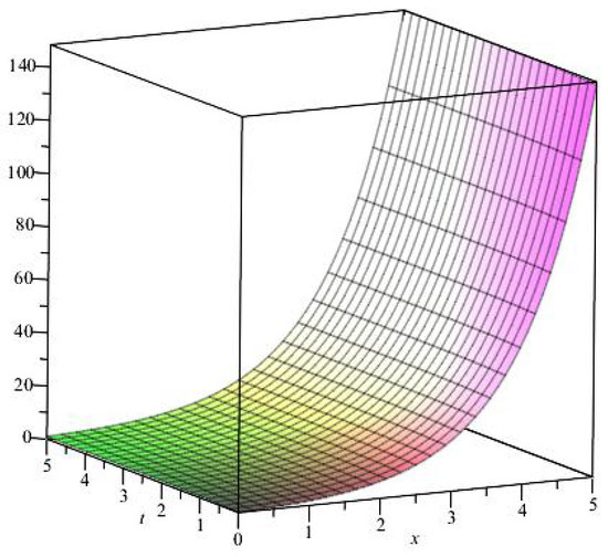
Figure 1. Values of the options for $\alpha =\rho =1$.

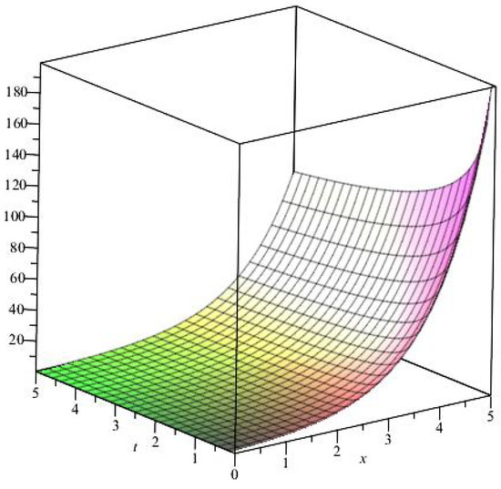
Figure 2. Values of the options for $\alpha =0.8$ and $\rho =1$.

Note that the analytic solution of the fractional Black-Scholes equation and the analytic solution of the classical Black-Scholes equation are in good agreement.

We observe that the value of $\rho$ has an effect on the diffusion process given in Table 1. If $\rho <1,$ then the parameter $\rho$ has an acceleration effect in the diffusion process. On the other hand, if $\rho >1,$ then the parameter $\rho$ has a retardation effect in the diffusion process. We observe a slight delay in the cost of the European option in the case of $\rho >1$. Therefore, $\rho$ impacts the European option price.

Table 1. Values of the European option with the different values of $\rho$.

order ($\alpha$)	1	1	1	1	1
order ($\rho$)	0.6	0.8	1	1.2	1.5
rate (r)	0.03	0.03	0.03	0.03	0.03
volatility ($\sigma$)	0.01	0.01	0.01	0.01	0.01
time ($\tau$)	0.5	0.5	0.5	0.5	0.5
expiration price (E)	100	100	100	100	100
asset price( S)	100	100	100	100	100
maturity (T)	1	1	1	1	1
European call option (C)	21.32	3.29	0.49	0.077	0.0049

5. Conclusions

In this article, the existence of a solution was investigated for the time-fractional Black-Scholes with European option pricing models, which have been described by the Katugampola fractional derivative operator. We discussed the approximate analytic solutions of the time-fractional Black-Scholes option pricing models by using the generalized Laplace homotopy perturbation method. We also pointed out the error analysis of the proposed method. Not only did we obtain the approximate analytic solution of the fractional Black-Scholes equation in the Katugampola derivative sense in the form of the generalized Mittag-Leffler function, but also, we obtained the approximate analytic solutions of the classical Black-Scholes equation and the time-fractional Black-Scholes equation in the Riemann–Liouville derivative sense. Unfortunately, in the case of the Hadamard derivative operator, there is no solution. The successful applications of the proposed time-fractional Black-Scholes model prove that this model is in complete agreement with the corresponding explicit closed-form solution. Note that the classical Black-Scholes equation is recovered when the order $\alpha =\rho =1$. Moreover, we observe that the value of $\rho$ has an effect in the cost of the European option. If $\rho >1$, then the order $\rho$ of the Katugampola derivative operator has a retardation in the diffusion process. Thus, we note a decrease in the cost of the European option. On the other hand, if $\rho <1$, then the order $\rho$ of the Katugampola derivative operator has an acceleration effect in the diffusion process. Thus, an increase in the European option cost is shown in Table 1. The numerical schemes of the fractional Black-Scholes equation with the Katugampola derivative operator will be the subject of future investigations in a forthcoming paper.

References

- Black, F.; Scholes, M. The pricing of options and corporate liabilities. J. Polit. Econ. 1973, 81, 637–654. [Google Scholar] [CrossRef]
- Owoloko, E.A.; Okeke, M.C. Investigating the Imperfection of the B–S Model: A Case Study of an Emerging Stock Market. Br. J. Appl. Sci. Tech. 2014, 4, 4191–4200. [Google Scholar] [CrossRef]
- Mandelbrot, B. The variation of certain speculative prices. J. Bus. 1963, 36, 394–413. [Google Scholar] [CrossRef]
- Peters, E.E. Fractal structure in the capital markets. Financ. Anal. J. 1989, 45, 32–37. [Google Scholar] [CrossRef]
- Li, H.Q.; Ma, C.Q. An empirical study of long-term memory of return and volatility in Chinese stock market. J. Financ. Econ. 2005, 31, 29–37. [Google Scholar]
- Huang, T.F.; Li, B.Y.; Xiong, J.X. Test on the chaotic characteristic of Chinese futures market. Syst. Eng. 2012, 30, 43–53. [Google Scholar]
- Debnath, L. Recent applications of fractional calculus to science and engineering. Int. J. Math. Math. Sci. 2003, 2003, 753601. [Google Scholar] [CrossRef]
- He, J.H.; El-Dib, Y.O. Periodic property of the time-fractional Kundu–Mukherjee–Naskar equation. Results Phys. 2020, 19, 103345. [Google Scholar] [CrossRef]
- Noeiaghdam, S.; Dreglea, A.; He, J.; Avazzadeh, Z.; Suleman, M.; Fariborzi Araghi, M.A.; Sidorov, D.N.; Sidorov, N. Error Estimation of the Homotopy Perturbation Method to Solve Second Kind Volterra Integral Equations with Piecewise Smooth Kernels: Application of the CADNA Library. Symmetry 2003, 12, 1730. [Google Scholar] [CrossRef]
- Anjum, N.; He, J.H. Higher-order homotopy perturbation method for conservative nonlinear oscillators generally and microelectromechanical systems’ oscillators particularly. Int. J. Mod. Phys. B 2020, 34, 2050313. [Google Scholar] [CrossRef]
- Song, L. A semianalytical solution of the fractional derivative model and its application in financial market. Complexity 2018, 2018, 1872409. [Google Scholar] [CrossRef]
- Edeki, S.O.; Ugbebor, O.O.; Owoloko, E.A. Analytical solutions of the Black–Scholes pricing model for european option valuation via a projected differential transformation method. Entropy 2015, 17, 7510–7521. [Google Scholar] [CrossRef]
- Smeureanu, I.; Fanache, D. A Linear Algorithm for Black–Scholes Economic Model. Rev. Inform. Econ. 2008, 1, 150–156. [Google Scholar]
- Wilmott, P.; Howson, S.; Howison, S.; Dewynne, J. The Mathematics of Financial Derivatives: A Student Introduction; Cambridge University Press: Cambridge, UK, 1995. [Google Scholar]
- Sawangtong, P.; Trachoo, K.; Sawangtong, W.; Wiwattanapataphee, B. The Analytical Solution for the Black-Scholes Equation with Two Assets in the Liouville-Caputo Fractional Derivative Sense. Mathematics 2018, 8, 129. [Google Scholar] [CrossRef]
- Kumar, S.; Yildirin, A.; Khan, Y.; Jafari, H.; Sayevand, K.; Wei, L. Analytical solution of fractional Black-Scholes European option pricing equations using Laplace transform. J. Frac. Cal. Appl. 2012, 2, 1–9. [Google Scholar]
- Kumar, S.; Kumar, D.; Singh, J. Numerical computation of fractional Black-Scholes equation arising in financial market. Egypt. J. Basic Appl. Sci. 2014, 1, 177–183. [Google Scholar] [CrossRef]
- Yavuz, M.; Özdemir, N. European vanilla option pricing model of fractional order without singular kernel. Fractal Fract. 2018, 2, 3. [Google Scholar] [CrossRef]
- Yavuz, M. European option pricing models described by fractional operators with classical and generalized Mittag Leffler kernels. Numer. Methods Partial. Differ. Equ. 2020. [Google Scholar] [CrossRef]
- Fall, A.N.; Ndiaye, S.N.; Sene, N. Black–Scholes option pricing equations described by the Caputo generalized fractional derivative. Chaos Solitons Fractals 2019, 125, 108–118. [Google Scholar] [CrossRef]
- Ahmad, J.; Shakee, Q.M.; Hassan, U.I.; Mohyud-Din, S.T. Analytical solution of Black-Scholes model using fractional variational iteration method. Int. J. Mod. Math. Sci. 2013, 5, 133–142. [Google Scholar]
- Blanco-Cocom, L.; Estrella, A.G.; Avila-Vales, E. Solution of the Black-Scholes equation via the Adomian decomposition method. Int. J. Appl. Math. Res. 2013, 2, 486–494. [Google Scholar]
- Sripacharasakullert, P.; Sawangtong, W.; Sawangtong, P.; Wiwattanapataphee, B. An approximate analytical solution of the fractional multi-dimensional Burgers equation by the homotopy perturbation method. Adv. Differ. Equa. 2019, 1, 1–12. [Google Scholar] [CrossRef]
- Trachoo, K.; Sawangtong, W.; Sawangtong, P. Laplace Transform Homotopy Perturbation Method for the Two Dimensional Black Scholes Model with European Call Option. Math. Comp. Appl. 2017, 1, 23. [Google Scholar] [CrossRef]
- Sawangtong, W.; Sawangtong, P. Green’s function homotopy perturbation method for the initial-boundary value problems. Adv. Differ. Equ. 2019, 1, 419. [Google Scholar] [CrossRef]
- Katugampola, U.N. A new approach to generalized fractional derivatives. arXiv 2011, arXiv:1106.0965. [Google Scholar]
- Jarad, F.; Abdeljawad, T. Generalized fractional derivatives and Laplace transform. Discret. Cont. Dyn. Syst. S 2019, 13, 709. [Google Scholar] [CrossRef]
- Sene, N.; Fall, A.N. Homotopy perturbation ρ-Laplace transform method and its application to the fractional diffusion equation and the fractional diffusion-reaction equation. Fractal Fract. 2019, 3, 14. [Google Scholar] [CrossRef]
- Kilbas, A.A.; Srivastava, H.M.; Trujillo, J.J. Theory and applications of fractional differential equations. In North-Holland Mathematics Studies; Elsevier Science B.V.: Amsterdam, The Netherlands, 2006; Volume 204. [Google Scholar]
- Garrappa, R.; Popolizio, M. Generalized exponential time differencing methods for fractional order problems. Comput. Math. Appl. 2011, 62, 876. [Google Scholar] [CrossRef]
- Ghorbani, A. Beyond Adomian polynomials: He polynomials. Chaos Solitons Fractals 2009, 39, 1486–1492. [Google Scholar] [CrossRef]
Publisher’s Note: MDPI stays neutral with regard to jurisdictional claims in published maps and institutional affiliations. |
© 2021 by the authors. Licensee MDPI, Basel, Switzerland. This article is an open access article distributed under the terms and conditions of the Creative Commons Attribution (CC BY) license (http://creativecommons.org/licenses/by/4.0/).