
The Relativistic Harmonic Oscillator in a Uniform Gravitational Field


Instituto Universitario de Matemática Multidisciplinar, Universitat Politècnica de Valencia, Camino de Vera, s/n, 46022 Valencia, Spain
Mathematics 2021, 9(4), 294; https://doi.org/10.3390/math9040294
Submission received: 9 January 2021
/
Revised: 28 January 2021
/
Accepted: 1 February 2021
/
Published: 3 February 2021
(This article belongs to the Special Issue Mathematical Methods, Modelling and Applications)
Abstract
:We present the relativistic generalization of the classical harmonic oscillator suspended within a uniform gravitational field measured by an observer in a laboratory in which the suspension point of the spring is fixed. The starting point of this analysis is a variational approach based on the Euler–Lagrange formalism. Due to the conceptual differences of mass in the framework of special relativity compared with the classical model, the correct treatment of the relativistic gravitational potential requires special attention. It is proved that the corresponding relativistic equation of motion has unique periodic solutions. Some approximate analytical results including the next-to-leading-order term in the non-relativistic limit are also examined. The discussion is rounded up with a numerical simulation of the full relativistic results in the case of a strong gravity field. Finally, the dynamics of the model is further explored by investigating phase space and its quantitative relativistic features.
Keywords:
relativistic harmonic oscillator; kinematics of a particle; special relativity; nonlinear problems in mechanics; equations of motion in gravitational theoryMSC:
70B05; 83A05; 70K42; 70K99; 83C101. Introduction
The harmonic oscillator or mechanical spring, implementing Hooke’s Law, is one of the standard textbook examples for introducing the student to Newtonian mechanics [1]. Treating classical motion under a Hookean potential is simplest, in spite of additional difficulties when, e.g., velocity-dependent forces (as friction) are added. Remarkably, the relativistic counterpart of an oscillator or a pendulum—which approximates to a harmonic oscillator for small amplitudes—stationed within some supplementary force field has so far been dealt with only scarcely.
A detailed discussion of relativistic effects on a simple pendulum without any additional forces has been carried out by Erkal in 2000 [2]. In 2008, Torres shows that the relativistic pendulum with friction possesses periodic solutions which are absent in the classical case [3]. In a more recent publication of this area of research, in 2017, de la Fuente and Torres focuses on relativistic extensions for the motion of the harmonic oscillator from the view of the oscillating body, but without including any gravitational effects [4]. In all these publications an appropriate laboratory frame is chosen where characteristic, preferred points are fixed, i.e., the suspension points of the pendulum and the spring representing the oscillator, respectively.
The present work fills an outstanding gap in the existing research literature by examining the relativistic effects of a harmonic oscillator in a uniform gravitational field, adopting and extending the approach by Goldstein and Bender [5]. In the classical model, the maximum velocity of the mass in motion can be arbitrarily large depending on the displacement with respect to the equilibrium point of the spring. Relativistic mechanics will adjust this behavior by only allowing a maximum speed less than the speed of light, as accelerating a mass to higher velocities will in like manner increase its inertial mass (equivalent to an increase in kinetic energy). Although the oscillating mass point is not considered to generate its own gravitational field and the uniform gravitational field shall be caused by an external object, any variable inertial mass will also be subject to gravity. This will inescapably lead to further nontrivial complications when studying relativistic effects of gravity for the harmonic oscillator—even from the perspective of special relativity without considering general relativity. Nonetheless, the present model may provide a legitimate and satisfactory approximation for an oscillator close to a black hole, as on a small scale the Schwarzschild spacetime at a sufficiently large distance from the event horizon (where gravitational tidal effects can be ignored) approximates well a strong uniform gravitational field.
The core of this paper is organized as follows. In Section 2, after a short introduction to the variational principle [6,7] for the classical case of the harmonic oscillator, the Euler–Lagrange formalism in the framework of special relativity [8,9] is used to set up the equations of motion for a harmonic oscillator which will be subject to an external uniform gravitational field and measured by an observer in a laboratory where the suspension point of the spring is fixed. Generalizing from the classical to the relativistic regime is not as trivial as it appears at first sight due to the particular, distinct nature of relativistic mass—mass which attains a dynamical quality—and the fact that variable kinetic energy itself is equivalent to additional mass which is susceptible to the external gravitational field. Special care has to be taken to take these entirely relativistic effects into account.
Therefore, Section 3 concentrates on the full derivation of the correct relativistic potential for the uniform gravitational field surrounding the harmonic oscillator. As approximation in the case of weak gravitational fields, we consider the Taylor expansion of the potential in the non-relativistic limit and some of its particular properties. Furthermore, we examine the full relativistic results for the potential with strong gravity and, in particular, identify its physically allowed regions. Although we are able to derive the relativistic gravitational potential for the case at hand, and in closed analytical form, the final results for the equation of motion become intangible for analytical evaluation.
In Section 4, we perform the numerical integration of the equation of motion to simulate the dynamics of this model and explore some significant characteristics of the system. In general, we prove that the equation of motion for the relativistic harmonic oscillator also has unique periodic solutions. In the strong gravity case, we compare relativistic with classical estimates for the oscillating amplitudes. For further analysis, we present the corresponding phase-space trajectories and discuss its most prominent characteristics.
2. Variational Principle and Equation of Motion
Robert Hooke (1635–1703) first pointed out that the mathematical description for small oscillations of a body with mass attached to an elastic spring with position takes the form: . The positive constant depends on the elastic properties of the spring in question. As a natural length scale serves the length of the spring at its maximum elongation, denoted as . This mechanical system is termed “harmonic oscillator”. Such systems are of utmost relevance in physics and engineering, as any mass particle subject to a force in stable equilibrium will effectively operate as a harmonic oscillator for small fluctuations—small fluctuations being displacements with only a fraction of length ℓ. Additional importance emerges in the dynamics of a continuous classical field as it may be formulated as the dynamics of an infinite number of harmonic oscillators. Furthermore, the quantum harmonic oscillator describes some of the most important model systems in quantum mechanics.
Already for the elementary classical case of a spring extended in a uniform Newtonian gravitational field, the most efficient and powerful approach is the framework of Lagrangian mechanics [6,7], which is based on a variational principle. Accordingly, the deterministic equations of motion will result from the following principle of least action
by varying over all possible paths and keeping the end points fixed. From Equation (1), it becomes clear that we exclude the oscillating mass point (which has negligible mass) as possible source of a gravitational field. For practical purposes and as is customary, the position x of the mass point and the external uniform gravitational field with strength are measured in the laboratory frame, where the suspension of the spring at one end is fixed.
The integrand in Equation (1) is the Lagrangian function, L, which includes kinetic energy , the spring potential , and the gravitational potential . Note that we consider spring elongations with respect to position which is also the suspension point of the spring. In this laboratory frame, with the suspension point at rest, the oscillating device is stationed within a uniform gravitational field (determined by the gravitational constant ) in such a way that both are aligned. This dynamical system is one-dimensional, and the corresponding Euler–Lagrange equation amounts to solving a simple linear second-order differential equation deriving from
By substituting the Lagrangian L from Equation (1) into Equation (2), it is straightforward to reproduce the well-known general solution in closed analytical form:
where and are the two integration constants depending on the initial values for the differential equation.
However, the classical result, Equation (3), does not contemplate strong gravitational fields and when velocities get closer to the speed of light . Furthermore, in special relativity the mass is a dynamical quantity, dependent on the relative velocity of the observer, such that , where the usual relativistic factor is . Consequently, Equation (3) will utterly fail in giving a faithful description of the physical effects in the relativistic domain.
In order to generalize to a correct description in the relativistic domain, the best starting point is to modify the classical principle of least action, Equation (1). As expected, the rest mass in Equation (1) will have to be divided by the factor to correctly incorporate both rest mass and kinetic energy. Moreover, the spring potential is unaltered, and the relativistic gravitational potential , however, is hitherto undetermined. Therefore, we postulate the relativistic Lagrangian
which readily yields the relativistic action principle
Note that , as stressed before, gives the relativistic gravitational potential as measured in the laboratory frame with fixed strength and as a function of varying spring elongation x.
Complications for identifying in Equation (5) arise, because mass in special relativity will change with its variable kinetic energy and thus simultaneously cause a change of the mass which is subject to the external gravitational field. This effect can be taken into account by using the relativistic ansatz
For a rigorous general definition of this potential see Goldstein & Bender [5].
As , and thus L, do not explicitly depend on time, according to Noether’s theorem total energy must be conserved. For this purpose, we carry out the Legendre transformation [6,7] of Equation (4) yielding the Lagrangian energy function
which is just the constant total energy E of the system. Without loss of generality, but for convenience, we assume for the remainder of the derivation that at position the mass particle be at rest, i.e., , or equivalently, we will assume that the following initial conditions hold:
Furthermore, this immediately implies via Equation (7) that
Observe that condition Equation (9) is chosen to agree with the definition of the classical potential and is nothing more than just fixing the arbitrary, and unphysical, integration constant in Equation (6).
Applying the Euler–Lagrange formalism to Equation (5) produces the following relativistic equation of motion,
where is still unknown and needs to be determined. The next section focuses on uncovering the explicit relativistic form of gravitational potential .
3. Relativistic Potential for Uniform Gravitational Field
As already stressed, the problem of dealing with the relativistic model of the harmonic oscillator in a uniform gravitational field is appreciably more complicated than the classical case. The core problem originates from the fundamentally different concept of mass in the classical or the relativistic description of the physical phenomena. The ansatz for the gravitational potential given in Equation (6) naturally considers relativistic corrections of a mass in relative motion with respect to the laboratory.
Moreover, from energy conservation, viz. Equation (7), with , and from solving for the relativistic factor , it directly follows that
which constrains the physically admissible range of potential .
Now, substituting the relativistic factor of Equation (11) into Equation (6) gives the integral equation
or correspondingly, the differential equation
where we have considered integration condition Equation (9). Furthermore, we indicated the correct sign of gradient , since the gravitational force, , is oriented downwards the x-axis. It is important to notice that Equation (13) contains the constant , considering that obviously the elastic property of the spring affects the speed of the oscillating mass and enters via the relativistic factor . This is in full agreement with previous published results using a similar approach, e.g., for the relativistic pendulum with a gravitational potential energy also depending on length of the pendulum, viz. (see in [2], Equation (6)).
Equation (13) is an ordinary differential equation of type which can easily be solved. The solution is
with derivative
Some checks of Equation (15) are in order: Note that in the absence of any spring (), the result is recovered, which is in full agreement with the calculations by Goldstein and Bender [5]. As a consequence, the classical result, is obtained for , before the mass particle is set in motion, viz. Equation (8). Moreover, in the weak gravity domain (), to lowest order the gravitational force obviously has to be independent of spring constant k, and it is , with ℓ being the natural length scale of the spring, viz. Section 2. However, as gravity becomes stronger, the harmonic force will entangle with gravity in the potential due to the subtle relativistic effects already mentioned. To see this, we expand Equation (14) in a power series and obtain the expansion of up to first order in the dimensionless scale parameter :
Observe that the quantity is a Lorentz scalar, representing an invariant for all inertial frames. Obviously, the speed of light c is a Lorentz scalar, and g being an acceleration is measured the same in all inertial frames with relative motion to the rest/laboratory frame. Thus, the ratio is also invariant under Lorentz transformations.
In Equation (16), the term of order already contains spring constant k. Therefore, in first approximation for weak gravity, the odd powers indicate a symmetric result, more precisely rotational symmetry with respect to rotations of 180 about the origin, see Figure 1. In the full relativistic regime, including all orders of the expansion, symmetry is broken. Observe also that in this expansion of the gravitational potential, the additional next-to-leading-order term represents the main correction of special relativity. It bears some similarity with the post-Newtonian approximation in general relativity. However, here in our approach—within the framework of special relativity—the underlying spacetime is of course Minkowskian, and thus flat.
Figure 2 displays the full relativistic result for in a strong gravitational field. Here, to achieve (measured in physical units m), all parameters are set to unity, except for the spring constant which we chose to be (measured in physical units kg/s). We also represent the gradient, , for any position . Note that the gravitational force therefore will flip sign at , satisfying for Equation (13), and is given by
where is the principal branch of Lambert’s W function (see in [10], §4.13). By including higher orders up to in Equation (16), a reasonably good approximation for Equation (17) is obtained: .
4. Model Dynamics and Numerical Simulation
With the exact analytical result for the relativistic gravitational potential , given by Equation (14), we are now in the position to complete the description of the dynamics of the model at hand. Substituting its derivative , given by Equation (15), into the equation of motion, Equation (10), readily yields the Euler–Lagrange equation—a nonlinear second-order differential equation—which governs the physical system
where and can be eliminated via Equations (11) and (14), respectively. After some lengthy but straightforward simplification, we arrive at the following equivalent and for numerical implementation more convenient form
where is given by Equation (14). Observe that are dimensionless factors, and in particular it is , such that at the initial position , as is expected. Furthermore, we obtain at all positions, when and . This represents the non-relativistic case in the absence of harmonic forces, that is, classical free fall. Similarly, for and , it is easily checked that the result reduces to that of a classical spring in a gravitational field: with general solutions Equation (3). Anyhow, Equations (19a) and (19b) embraces the full relativistic case provided that constraint Equation (11) is satisfied. The constraint Equation (11) may simply be rewritten as
Therefore, the physically relevant gravitational potential always has to lie below this concave down parabola. Figure 2 shows that this will approximately hold for the range , where no sign-flip for the gravitational force occurs. Recall that with the aforementioned parameters (all set to unity except for kg/s2), we found m, viz. Equation (17).
The particular structure of the relativistic equation of motion, Equations (19a) and (19b), also implies existence and uniqueness of periodic solutions. During the past two decades, considerable progress has been made in the study of second-order differential equations and the periodic properties of their solutions [11]. For a closer analysis, we recast Equation (19a) into the form
where in this case the continuous function f (assuming ) does not explicitly depend on the variables t or . Moreover, recall that . To guarantee existence and uniqueness, we have to check that is bounded by two continuous functions for all , with period [11]. For this purpose, we also use the following general results for the limits of Equation (19b) and its derivatives:
Now, we can conclude that
As and are continuous, necessarily has to be bounded by a lower and an upper continuous function for , and we affirm that the equation of motion, Equations (19a) and (19b), has unique periodic solutions.
The series expansion in the non-relativistic limit of Equations (19a) and (19b) up to first order in the dimensionless parameter gives
and analytical integration is possible but will already yield a rather convoluted list of elliptic integrals. Therefore, for the full relativistic result—including all higher orders—numerical integration is the most appropriate, if not the only possible, open pathway.
For the actual numerical integration of Equations (19a) and (19b), we decided to implement the code in the Julia programming language due to its efficiency and high performance [12]. Figure 3 displays the computed amplitudes for the classical and relativistic case over the time interval in SI units of seconds, again with all parameters set equal to unity, except for the spring constant kg/s2. Using the Julia library DifferentialEquations.jl [13], we chose the algorithm based on first-order interpolation with at least stepsize s and a relative tolerance of in the adaptive timestepping. Note that a long-time analysis has shown that no significant numerical errors materialize.
As shown in Figure 3, the difference between the simple classical result, resulting from Equation (3) with conditions Equation (8),
and the relativistic numerical estimate is quite pronounced—not only in amplitude but also in phase, with a positive phase shift. The physical results for the relativistic oscillator always possess longer amplitude and period than the classical analogue by cause of the relativistic mass increase.
For an extended time interval in units of seconds, Figure 4 shows the difference between relativistic and classical predictions, , as already individually shown in Figure 3. As found before from the two curves in Figure 3, the relativistic corrections—now more easily recognized—propagate with a positive phase while significantly modulating the amplitude of the classical model. These contributions are substantial and cannot be neglected. Remarkably, these relativistic corrections take the shape of pronounced wave packets.
Figure 5 depicts the phase space for the relativistic harmonic oscillator with potential in comparison with the classical model, using the same parameters as before, viz. Figure 2. This phase portrait provides a global overview about the dynamics of the oscillating system and shows the quantitative difference between the two models.
The relativistic phase-space trajectories emerge from the equation of motion, Equation (18), with the preserved quantity
which represents energy conservation with total energy in Equation (7). In the non-relativistic limit, we may use and in Equation (26) to obtain
which is just the well-known result for the harmonic oscillator with uniform Newtonian gravity.
The classical solutions are then reproduced in the phase plane as the level curves of Equation (27) by varying . Similarly, we obtain the relativistic solutions in the phase plane by drawing the level curves of Equation (26). With the chosen initial conditions in Equation (8), we have for both cases (which is equivalent to ). Figure 5 shows the two corresponding curves. Observe that Equations (26) and (27) always produce phase-space trajectories (relativistically and classically) which are closed. As a consequence, both types of solutions have to be periodic. The phase portraits of both cases represent center stable dynamics. Another characteristic effect is that the phase-space path for the relativistic case is larger than for the classical path—an effect which also has been observed for the relativistic pendulum [2] and a harmonic oscillator satisfying a relativistic isochronicity principle [4].
5. Conclusions
We have derived and studied the relativistic generalization of an oscillating body in motion under a Hookean potential and in parallel alignment with a uniform gravitational field.
If gravity is strong, these relativistic corrections differ substantially from the classical predictions and are relevant. These amplitude corrections can be pictured as fluctuating wave packets traveling on top of the classically predicted oscillations.
Quantitatively, the relativistic oscillator always acquires longer amplitudes and periods than the classical analogue. This is the dynamical effect due to the increase in mass of a moving object as dictated by special relativity. In spite of this fundamental difference between the relativistic and non-relativistic framework, we have proven that the corresponding relativistic equation of motion still maintains unique periodic solutions, similar to the well-known classical case.
For practical purposes, we have also presented approximations in the non-relativistic limit (keeping the next-to-leading-order term) for the relativistic gravitational potential and for the equation of motion of the harmonic oscillator—an approximate equation which could still be solved analytically in terms of elliptic integrals. However, all estimates in the fully relativistic regime have to be solved by numerical integration. Toward this end, we implemented the integration code with high precision in the Julia programming language by using efficient first-order interpolation. This simulation also allowed to represent the classical and relativistic phase space and to explore the dynamics of both models with their common and quantitatively different features.
Funding
This work has been supported by the Spanish Ministerio de Economía y Competitividad, the European Regional Development Fund (ERDF) under grant TIN2017-89314-P, and the Programa de Apoyo a la Investigación y Desarrollo 2018 (PAID-06-18) of the Universitat Politècnica de València under grant SP20180016.
Institutional Review Board Statement
Not applicable.
Informed Consent Statement
Not applicable.
Data Availability Statement
Not applicable.
Conflicts of Interest
The author declares no conflict of interest.
References
- Goldstein, H.; Poole, C.; Safko, J. Classical Mechanics; Addison Wesley: Boston, MA, USA, 2001. [Google Scholar]
- Erkal, C. The simple pendulum: A relativistic revisit. Eur. J. Phys. 2000, 21, 377–384. [Google Scholar] [CrossRef]
- Torres, P.J. Periodic oscillations of the relativistic pendulum with friction. Phys. Lett. A 2008, 372, 6386–6387. [Google Scholar] [CrossRef]
- de la Fuente, D.; Torres, P.J. A new relativistic extension of the harmonic oscillator satisfying an isochronicity principle. Qual. Theory Dyn. Syst. 2017, 34, 579–589. [Google Scholar] [CrossRef]
- Goldstein, H.F.; Bender, C.M. Relativistic brachistochrone. J. Math. Phys. 1986, 27, 507–511. [Google Scholar] [CrossRef]
- Lanczos, C. The Variational Principles of Mechanics; Dover Publications: New York, NY, USA, 1970. [Google Scholar]
- Mann, P. Lagrangian and Hamiltonian Dynamics; Oxford University Press: Oxford, UK, 2018. [Google Scholar]
- Christodoulides, C. The Special Theory of Relativity: Foundations, Theory, Verification, Applications; Springer: New York, NY, USA, 2016. [Google Scholar]
- Rahaman, F. The Special Theory of Relativity: A Mathematical Approach; Springer: Berlin/Heidelberg, Germany, 2014. [Google Scholar]
- Olver, F.J.W.; Lozier, D.W.; Boisvert, R.F.; Clark, C.W. NIST Digital Library of Mathematical Functions; National Institute of Standards and Technology: Gaithersburg, MD, USA, 2020; Release 1.0.27 of 2020-06-15; Section 4.13: Lambert W-Function. Available online: https://dlmf.nist.gov/4.13 (accessed on 9 January 2021).
- Wei, Y. Existence and Uniqueness of Periodic Solutions for Second Order Differential Equations. J. Funct. Spaces 2014, 2014, 246258. [Google Scholar] [CrossRef]
- Bezanson, J.; Edelman, A.; Karpinski, S.; Shah, V.B. Julia: A fresh approach to numerical computing. SIAM Rev. 2017, 59, 65–98. [Google Scholar] [CrossRef] [Green Version]
- Rackauckas, C.; Nie, Q. DifferentialEquations.jl—A performant and feature-rich ecosystem for solving differential equations in Julia. J. Open Res. Softw. 2017, 5, 15. [Google Scholar] [CrossRef] [Green Version]
Figure 1.
In the weak gravity case, when , the approximation for the relativistic gravitational potential in the non-relativistic limit is most suitable (blue curve), see Equation (16). This approximate result is symmetric with respect to rotations of 180 about the origin—a symmetry property which is lost in the full relativistic case. The approximate model is only physically valid well within the interval , where , so that sign-flips of the force field are avoided. The non-relativistic, classical case is indicated by the straight gray line.
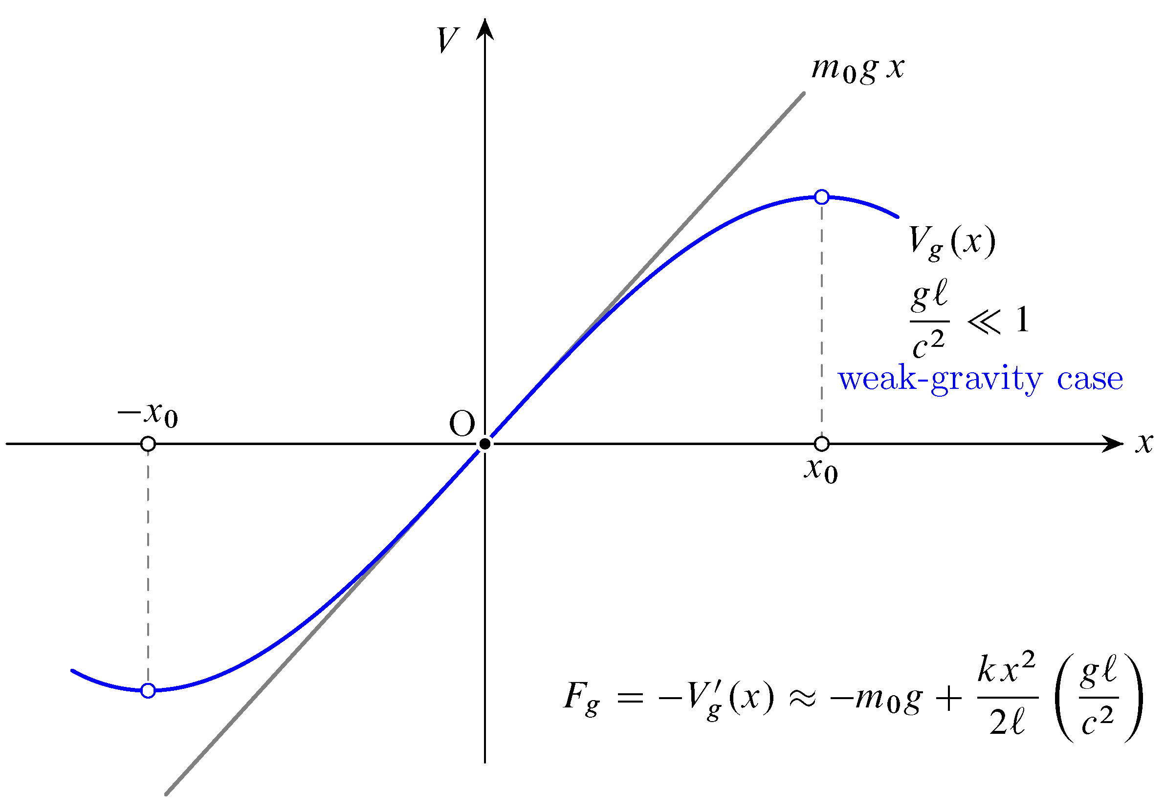
Figure 2.
The relativistic gravitational potential, , for an oscillating body posted in a strong uniform gravitational field. For the graphical representation we use kg, kg m/s, and kg/s. Further, the speed of light is normalized to m/s. The dashed line marks below the physically allowed region for , viz. Equation (20). The gradient, , is also shown.

Figure 3.
Amplitudes for the relativistic harmonic oscillator compared to the classical model, both suspended in a uniform gravitational field, either using the simple classical solution, viz. Equation (3), or the relativistic estimates resulting by numerical integration of Equations (19a) and (19b). The gravitational field is strong with m−1, choosing again all parameters unity, except for kg/s, see Figure 2. The two initial conditions are , see Equation (8).

Figure 4.
Amplitude changes, , characterizing the relativistic corrections for the classical harmonic oscillator in a strong uniform gravitational field, corresponding to the physical configuration of Figure 3, but for the larger time interval in units of seconds. These corrections are significant and modulate in both amplitude and phase.

Figure 5.
The phase-space diagrams for the harmonic oscillator in a uniform gravitational field corresponding to the classical and the relativistic case. We are using the same parameters as in Figure 2. The characteristics for both cases are similar: the closed trajectories represent periodic solutions, and their phase portraits represent center stable dynamics.

Publisher’s Note: MDPI stays neutral with regard to jurisdictional claims in published maps and institutional affiliations. |
© 2021 by the author. Licensee MDPI, Basel, Switzerland. This article is an open access article distributed under the terms and conditions of the Creative Commons Attribution (CC BY) license (http://creativecommons.org/licenses/by/4.0/).
Share and Cite
MDPI and ACS Style
Tung, M.M. The Relativistic Harmonic Oscillator in a Uniform Gravitational Field. Mathematics 2021, 9, 294. https://doi.org/10.3390/math9040294
AMA Style
Tung MM. The Relativistic Harmonic Oscillator in a Uniform Gravitational Field. Mathematics. 2021; 9(4):294. https://doi.org/10.3390/math9040294
Chicago/Turabian StyleTung, Michael M. 2021. "The Relativistic Harmonic Oscillator in a Uniform Gravitational Field" Mathematics 9, no. 4: 294. https://doi.org/10.3390/math9040294
Note that from the first issue of 2016, this journal uses article numbers instead of page numbers. See further details here.