Optimal Reinsurance Problem under Fixed Cost and Exponential Preferences

Abstract

We investigate an optimal reinsurance problem for an insurance company taking into account subscription costs: that is, a constant fixed cost is paid when the reinsurance contract is signed. Differently from the classical reinsurance problem, where the insurer has to choose an optimal retention level according to some given criterion, in this paper, the insurer needs to optimally choose both the starting time of the reinsurance contract and the retention level to apply. The criterion is the maximization of the insurer’s expected utility of terminal wealth. This leads to a mixed optimal control/optimal stopping time problem, which is solved by a two-step procedure: first considering the pure-reinsurance stochastic control problem and next discussing a time-inhomogeneous optimal stopping problem with discontinuous reward. Using the classical Cramér–Lundberg approximation risk model, we prove that the optimal strategy is deterministic and depends on the model parameters. In particular, we show that there exists a maximum fixed cost that the insurer is willing to pay for the contract activation. Finally, we provide some economical interpretations and numerical simulations.

1. Introduction

The insurance business requires the transfer of risks from the policyholders to the insurer, who receives a risk premium as a reward. In some cases, it could be convenient to cede these risks to a third party, which is the reinsurance company. From the operational viewpoint, a risk-sharing agreement helps the insurer reducing unexpected losses, stabilizing operating results, increasing business capacity and so on. By means of a reinsurance treaty, the reinsurance company agrees to indemnify the primary insurer (cedent) against all or part of the losses which may occur under policies which the latter issued. The cedent will pay a reinsurance premium in exchange for this service. Roughly speaking, this is an insurance for insurers. When subscribing a reinsurance treaty, a natural question is to determine the (optimal) level of the retained losses. Optimal reinsurance problems have been intensively studied by many authors under different criteria, especially through expected utility maximization and ruin probability minimization (see, e.g., [1,2,3,4,5,6] and references therein).

The main novelty of this article is that subscription costs are considered. Transaction costs represent the bureaucratic fixed costs necessary to run and manage an insurance company. The empirical impact of these costs on insurances choices has been highlighted in the actuarial literature (see, e.g., [7,8]). In practice, in the reinsurance context, when the agreement is signed, a fixed cost is usually paid in addition to the reinsurance premium. This aspect has not been investigated by nearly all the studies, except for those in [9,10]. In the former work, the authors discussed the reinsurance problem subject to a fixed cost for buying reinsurance and a time delay in completing the reinsurance transaction. They solved the problem considering a performance criterion with linear current reward and showed that it is optimal to buy reinsurance when the surplus lies in a bounded interval depending on the delay time. In the latter paper, under the criterion of minimizing the ruin probability, the original problem is reduced to a time-homogeneous optimal stopping problem. In particular, the authors showed that the fixed cost forces the insurer to postpone buying reinsurance until the surplus process hits a certain level.

Hence, the presence of a fixed cost is closely related to the possibility of postponing the subscription of the reinsurance agreement. This, in turn, involves an optimal stopping problem, which is attached to the optimal choice of the retention level, which is a well known stochastic control problem. The novelty of our paper consists in considering this mixed stochastic control problem under the criterion of maximizing the expected utility of terminal wealth. The strategy of the insurance company consists of the retention level of a proportional reinsurance and the subscription timing. When the contract is signed, a given fixed cost is paid and the optimal retention level is applied. For the purpose of mathematical tractability, we use a diffusion approximation to model the insurer’s surplus process (see [11]). The insurance company has exponential preferences and is allowed to invest in a risk-less bond.

As already mentioned, this setup leads to a combined problem of optimal stopping and stochastic control with finite horizon, which we solve by a two-step procedure. For theoretical studies on mixed control-stopping problems, we refer to, e.g., the works in [12,13,14]. First, we provide the solution of the pure reinsurance problem (with starting time equal to zero). Next, we discuss an optimal stopping time problem with a suitable reward function depending on the value function of the pure reinsurance problem. Differently to the works in [9,10], the associated optimal stopping problem turns out to be time-inhomogeneous and with discontinuous stopping reward with respect to the time. We provide an explicit solution, also showing that the optimal stopping time is deterministic. Moreover, we find that there are only two possible cases, depending on the model parameters. When the fixed cost is greater than a suitable threshold (whose analytical expression is available), the optimal choice is not to subscribe the reinsurance; otherwise, the insurer immediately subscribes the contract.

A recent related research can be found in [15] (see also references therein), where the problem of optimal dividends and reinsurance is formulated as a mixed classical-impulse stochastic control problem. The authors considered a fixed transaction cost when the dividends are paid out and solved the problem using the method of quasi-variational inequalities.

The paper is organized as follows. In Section 2, we describe the model and formulate the problem as a mixed stochastic control problem, i.e., a problem which involves both optimal control and stopping. In Section 3, we discuss the pure reinsurance problem (without stopping) by solving the associated Halmilton–Jacobi–Bellman equation. Section 4 is devoted to the reduction of the original (mixed) problem to a suitable optimal stopping problem, which is then investigated in Section 5. Here, we provide a verification theorem and solve the associated variational inequality. In Section 6, we give the explicit solution to the original problem and we discuss some economic implications of our results. Finally, in Section 7, some numerical simulations are performed in order to better understand the economic interpretation of our findings.

2. Problem Formulation

2.1. Model Formulation

Let $T>0$ be a finite time horizon and assume that $(\mathsf{\Omega },\mathcal{F},\mathbb{P},\mathbb{F})$ is a complete probability space endowed with a filtration $\mathbb{F}\doteq {\left\{{\mathcal{F}}_t\right\}}_{t\in [0,T]}$ satisfying the usual conditions.

Let us denote by $R={\left\{R_t\right\}}_{t\in [0,T]}$ the surplus process of an insurance company. There is a wide range of risk models in the actuarial literature (see, e.g., [11,16]). In the Cramér–Lundberg risk model, the claims arrival times are described by the sequence of claims arrival times ${\left\{T_n\right\}}_{n\ge 1}$, with $T_n<T_{n+1}$$\mathbb{P}$-almost everywhere $\forall n\ge 1$, while the corresponding claim sizes are given by ${\left\{Z_n\right\}}_{n\ge 1}$. In particular, the number of occurred claims up to time $t\ge 0$ is equal to

$$N_t=\sum _{n=1}{\mathbb{𝟙}}_{\{T_n\le t\}},$$

and it is assumed to be a Poisson process with constant intensity $\lambda >0$, independent of the sequence ${\left\{Z_n\right\}}_{n\ge 1}$. Moreover, ${\left\{Z_n\right\}}_{n\ge 1}$ are independent and identically distributed random variables with common probability distribution function $F_Z\left(z\right)$, $z\in (0,+\infty )$, having finite first and second moments denoted by $\mu >0$ and ${\mu }_2>0$, respectively. In this context, the surplus process is given by

$$R_0+ct-\sum _{n=1}^{N_t}{Z}_n,R_0>0,$$

(1)

where $R_0$ is the initial capital and $c>0$ denotes the gross risk premium rate. We can show that for any $t\ge 0$

$$\mathbb{E}\left[\sum _{n=1}^{N_t}{Z}_n\right]=\lambda \mu t\mathrm{and}var\left[\sum _{n=1}^{N_t}{Z}_n\right]=\lambda {\mu }_{2}t.$$

In this paper, we use the diffusion approximation of the Cramér–Lundberg model (1) (see, e.g., [16]). Precisely, we assume that the surplus process follows this stochastic differential equation (SDE):

$$d{R}_t=pdt+{\sigma }_{0}d{W}_t,R_0>0,$$

where $W={\left\{W_t\right\}}_{t\in [0,T]}$ is a standard Brownian motion, ${\sigma }_0=\sqrt{\lambda {\mu }_2}$ and p denotes the insurer’s net profit, that is $p=c-\mu \lambda$. In particular, under the expected value principle (see, e.g., [11]), we have that $c=(1+{\theta }_i)\mu \lambda$ and hence $p={\theta }_i\mu \lambda$, with ${\theta }_i>0$ representing the insurer’s safety loading.

We allow the insurer to invest her surplus in a risk-free asset with constant interest rate $R>0$:

$$d{B}_t=B_{t}Rdt,B_0=1,$$

hence the wealth process $X={\left\{X_t\right\}}_{t\in [0,T]}$ evolves according to

$$d{X}_t=R{X}_{t}dt+pdt+{\sigma }_{0}d{W}_t,X_0=R_0>0.$$

(2)

The explicit solution of the SDE (2) is given by the following equation:

$$X_t=R_0{e}^{Rt}+{\int }_0^t{e}^{R(t-s)}pds+{\int }_0^t{e}^{R(t-s)}{\sigma }_{0}d{W}_s,t\in [0,T].$$

(3)

Now, let $\tau$ denote an $\mathbb{F}$-stopping time. At time $\tau$, the insurer can subscribe a proportional reinsurance contract with retention level $u\in [0,1]$, transferring part of her risks to the reinsurer. More precisely, u represents the percentage of retained losses, so that $u=0$ means full reinsurance, while $u=1$ is equivalent to no reinsurance. To buy a reinsurance agreement, the primary insurer pays a reinsurance premium $q\left(u\right)\ge 0$. When the reinsurance contract is signed at time $t=0$, the Cramér–Lundberg risk model (1) is replaced by the following equation:

$$R_0+(c-q\left(u\right))t-\sum _{n=1}^{N_t}u{Z}_n,R_0>0.$$

Under the expected value principle, we have that $q\left(u\right)=(1+\theta )(1-u)\mu \lambda$, $u\in [0,1]$, with the reinsurer’s safety loading $\theta$ satisfying $\theta >{\theta }_i$ (preventing the insurer from gaining a risk-free profit).

Let us denote by $R^u={\left\{R_t^u\right\}}_{t\in [0,T]}$ the reserve process in the Cramér–Lundberg approximation associated with a given reinsurance strategy ${\left\{u_t\right\}}_{t\in [0,T]}$ when the reinsurance contract is signed at time $t=0$. Following Eisenberg and Schmidli [17], under the expected value principle, $R^u$ follows

$$d{R}_t^u=(p-q+q{u}_t)dt+{\sigma }_0{u}_{t}d{W}_t,R_0^u=R_0,$$

(4)

where $q=\theta \lambda \mu$ denotes the reinsurer’s net profit. We set $q>p$ (non-cheap reinsurance). The wealth process under the strategy ${\left\{u_t\right\}}_{t\in [0,T]}$ evolves according to this SDE:

$$d{X}_t^u=R{X}_t^{u}dt+d{R}_t^u,X_0^u=R_0,$$

(5)

which admits this explicit representation:

$$X_t^u=R_0{e}^{Rt}+{\int }_0^t{e}^{R(t-s)}(p-q+q{u}_s)ds+{\int }_0^t{e}^{R(t-s)}{\sigma }_0{u}_{s}d{W}_s.$$

(6)

We assume that a constant fixed cost $K>0$ is paid when the reinsurance contract is subscribed. The insurer decides when the reinsurance contract starts and which retention level is applied. Hence, the insurer’s strategy is a couple $\alpha =(\tau ,{\left\{u_t\right\}}_{t\in [\tau ,T]})$, with $\tau \le T$. Let $H_t=I_{\{\tau \le t\}}$ be the indicator process of the contract starting time. For $\tau <T$$\mathbb{P}$-a.s., the total wealth $X^{\alpha }={\left\{X_t^{\alpha }\right\}}_{t\in [0,T]}$ associated with a given strategy $\alpha$ is given by

$$d{X}_t^{\alpha }=(1-H_t)d{X}_t+H_{t}d{X}_t^u-Kd{H}_t,X_0^{\alpha }=R_0>0,$$

(7)

while on the event $\{\tau =T\}$ we have that

$$d{X}_t^{\alpha }=d{X}_t,X_0^{\alpha }=R_0>0,$$

(8)

where X satisfies Equation (2).

Equation (7) can be written more explicitly as

$$d{X}_t^{\alpha }=\left\{\begin{array}{cc}d{X}_t,\hfill & t<\tau ,X_0=R_0,\hfill \\ d{X}_t^u,\hfill & \tau <t\le T,X_{\tau }^u=X_{\tau }-K,\hfill \end{array}\right.$$

(9)

where X and $X^u$ satisfy Equations (2) and (5), respectively.

In our setting, the null reinsurance corresponds to the choice $\tau =T$, $\mathbb{P}$-a.s., to which we associate the strategy ${\alpha }_{\mathrm{null}}=(T,1)$ and

$$X_t^{{\alpha }_{\mathrm{null}}}=X_t,t\in [0,T].$$

2.2. The Utility Maximization Problem

The insurers’ objective is to maximize the expected utility of the terminal wealth:

$$\underset{\alpha \in \mathcal{A}}{sup}\mathbb{E}\left[U\left(X_T^{\alpha }\right)\right],$$

(10)

where $U:\mathbb{R}\to [0,+\infty )$ is the utility function representing the insurer’s preferences and $\mathcal{A}$ the class of admissible strategies (see Definition 1).

We focus on CARA (Constant Absolute Risk Aversion) utility functions, whose general expression is given by

$$U\left(x\right)=1-e^{-\eta x},x\in \mathbb{R},$$

where $\eta >0$ is the risk-aversion parameter. This utility function is highly relevant in economic science and particularly in insurance theory. Indeed, it is commonly used for reinsurance problems (e.g., see [5] and references therein).

The optimization problem is a mixed optimal control problem. That is, the insurer’s controls involve the timing of the reinsurance contract subscription and the retention level to apply.

Definition 1

(Admissible strategies). We denote by $\mathcal{A}$ the set of admissible strategies $\alpha =(\tau ,{\left\{u_t\right\}}_{t\in [\tau ,T]})$, where τ is an $\mathbb{F}$-stopping time such that $\tau \le T$ and ${\left\{u_t\right\}}_{t\in [\tau ,T]}$ is an $\mathbb{F}$-predictable process with values in $[0,1]$. Let us observe that the null strategy ${\alpha }_{\mathrm{null}}=(T,1)$ is included in $\mathcal{A}$. When we want to restrict the controls to the time interval $[t,T]$, we use the notation ${\mathcal{A}}_t$.

Proposition 1.

Let $\alpha \in \mathcal{A}$, then

$$\mathbb{E}\left[e^{-\eta X_T^{\alpha }}\right]<+\infty .$$

Proof. 

Using Equations (6) and (9), we have that

$$\begin{array}{cc}\hfill \mathbb{E}\left[e^{-\eta X_T^{\alpha }}\right]& =\mathbb{E}\left[e^{-\eta X_T}{I}_{\{\tau =T\}}\right]\hfill \\ & +\mathbb{E}\left[e^{-\eta (X_{\tau }-K)e^{R(T-\tau )}}{e}^{-\eta {\int }_{\tau }^T{e}^{R(T-s)}(p-q+q{u}_s)ds}{e}^{-\eta {\int }_{\tau }^T{e}^{R(T-s)}{\sigma }_0{u}_{s}d{W}_s}{I}_{\{\tau <T\}}\right].\hfill \end{array}$$

Taking into account the expression (3), we get

$$\begin{array}{cc}\hfill \mathbb{E}\left[e^{-\eta X_T}{I}_{\{\tau =T\}}\right]& \le \mathbb{E}\left[e^{-\eta R_0{e}^{RT}}{e}^{-\eta {\int }_0^T{e}^{R(t-s)}pds}{e}^{-\eta {\int }_0^T{e}^{R(t-s)}{\sigma }_{0}d{W}_s}\right]\hfill \\ & \le \mathbb{E}\left[e^{-\eta {\int }_0^T{e}^{R(t-s)}{\sigma }_{0}d{W}_s}\right]\hfill \\ & =e^{\frac{{\eta }^2}{2}{\int }_0^T{e}^{2R(t-s)}{\sigma }_0^{2}ds}<+\infty ,\hfill \end{array}$$

and denoting by C a generic constant (possibly different from each line to another)

$$\begin{array}{cc}& \mathbb{E}\left[e^{-\eta (X_{\tau }-K)e^{R(T-\tau )}}{e}^{-\eta {\int }_{\tau }^T{e}^{R(T-s)}(p-q+q{u}_s)ds}{e}^{-\eta {\int }_{\tau }^T{e}^{R(T-s)}{\sigma }_0{u}_{s}d{W}_s}{I}_{\{\tau <T\}}\right]\hfill \\ & \le C\times \mathbb{E}\left[e^{-\eta (X_{\tau }-K)e^{R(T-\tau )}}{e}^{-\eta {\int }_{\tau }^T{e}^{R(T-s)}{\sigma }_0{u}_{s}d{W}_s}{I}_{\{\tau <T\}}\right]\hfill \\ & \le C\times \left(\mathbb{E}\left[e^{-2\eta (X_{\tau }-K)e^{2R(T-\tau )}}{I}_{\{\tau <T\}}\right]+\mathbb{E}\left[e^{-2\eta {\int }_{\tau }^T{e}^{R(T-s)}{\sigma }_0{u}_{s}d{W}_s}{I}_{\{\tau <T\}}\right]\right)\hfill \\ & \le C\times \left(\mathbb{E}\left[e^{-2\eta X_{\tau }{e}^{2R(T-\tau )}}\right]+\mathbb{E}\left[e^{-2\eta {\int }_{\tau }^T{e}^{R(T-s)}{\sigma }_0{u}_{s}d{W}_s}{I}_{\{\tau <T\}}\right]\right)\hfill \\ & \le C\times \left(\mathbb{E}\left[e^{-2\eta e^{2R(T-\tau )}{\int }_0^{\tau }{e}^{R(t-s)}{\sigma }_{0}d{W}_s}\right]+\mathbb{E}\left[e^{2{\eta }^2{\int }_{\tau }^T{e}^{2R(T-s)}{\sigma }_0^2{u}_s^2{I}_{\{\tau <T\}}ds}\right]\right)\hfill \\ & \le C\times \left(e^{2{\eta }^2{e}^{4RT}{\int }_0^T{e}^{2R(t-s)}{\sigma }_0^{2}ds}+e^{2{\eta }^2{\int }_0^T{e}^{2R(T-s)}{\sigma }_0^{2}ds}\right)<+\infty .\hfill \end{array}$$

□

Let us introduce the value function associated to our problem (10):

$$V(t,x)=\underset{\alpha \in {\mathcal{A}}_t}{inf}\mathbb{E}\left[e^{-\eta X_T^{\alpha ,t,x}}\right],(t,x)\in [0,T]\times \mathbb{R},$$

(11)

where $X^{\alpha ,t,x}={\left\{X_s^{\alpha ,t,x}\right\}}_{s\in [t,T]}$ denotes the wealth given in Equation (9) with initial condition $(t,x)\in [0,T]\times \mathbb{R}$, that is $X_t^{\alpha ,t,x}=x$. We notice that

$$V(T,x)=e^{-\eta x}\forall x\in \mathbb{R},$$

(12)

because $X_T^{\alpha ,T,x}=x$$\forall \alpha \in \mathcal{A}$.

3. The Pure Reinsurance Problem

To have a self-contained article, in this section, we briefly investigate a pure reinsurance problem, which corresponds to the problem (10) with fixed starting time $t=0$. Precisely, we deal with

$$\underset{u\in \mathcal{U}}{inf}\mathbb{E}\left[e^{-\eta X_T^u}\right],$$

where $\mathcal{U}$ denotes the class of admissible strategies $u={\left\{u_t\right\}}_{t\in [0,T]}$, which are all the $\mathbb{F}$-predictable processes with values in $[0,1]$. Let us denote by $\overline{V}(t,x)$ the value function associated to this problem, that is

$$\overline{V}(t,x)=\underset{u\in {\mathcal{U}}_t}{inf}\mathbb{E}\left[e^{-\eta X_T^{u,t,x}}\right],(t,x)\in [0,T]\times \mathbb{R},$$

(13)

with ${\mathcal{U}}_t$ denoting the restriction of $\mathcal{U}$ to the time interval $[t,T]$ and ${\left\{X_s^{u,t,x}\right\}}_{s\in [t,T]}$ denotes the process satisfying Equation (5) with initial data $(t,x)\in [0,T]\times \mathbb{R}$. It is well known that the value function (13) can be characterized as a classical solution to the associated Hamilton–Jacobi–Bellman (HJB) equation:

$$\left\{\begin{array}{cc}\underset{u\in [0,1]}{min}{\mathcal{L}}^u\overline{V}(t,x)=0\hfill & \forall (t,x)\in [0,T)\times \mathbb{R}\hfill \\ \overline{V}(T,x)=e^{-\eta x}\hfill & \forall x\in \mathbb{R},\hfill \end{array}\right.$$

(14)

where, using Equations (4) and (5), the generator of the Markov process $X^u$ is given by

$${\mathcal{L}}^{u}f(t,x)=\frac{\partial f}{\partial t}(t,x)+(Rx+p-q+qu)\frac{\partial f}{\partial x}(t,x)+\frac{1}{2}{\sigma }_0^2{u}^2\frac{{\partial }^{2}f}{\partial x^2}(t,x),f\in {\mathcal{C}}^{1,2}((0,T)\times \mathbb{R}),$$

with ${\mathcal{C}}^{1,2}((0,T)\times \mathbb{R})$ denoting the class of continuous functions, with continuous first-order partial derivative with respect to the first (time) variable and continuous second-order derivative with respect to the second (space) variable.

Under the ansatz $\overline{V}(t,x)=e^{-\eta x{e}^{R(T-t)}}\varphi \left(t\right)$, the HJB equation reads as

$${\varphi }^{\prime }\left(t\right)+\mathsf{\Psi }\left(t\right)\varphi \left(t\right)=0,\varphi \left(T\right)=1,$$

where

$$\mathsf{\Psi }\left(t\right)=\underset{u\in [0,1]}{min}\{-\eta e^{R(T-t)}(p-q+qu)+\frac{1}{2}{\sigma }_0^2{u}^2{\eta }^2{e}^{2R(T-t)}\}.$$

Solving the minimization problem, we find the unique minimizer:

$$u^{*}\left(t\right)=\frac{q}{\eta {\sigma }_0^2}{e}^{-R(T-t)}\vee 1,t\in [0,T].$$

Under the additional condition

$$q<\eta {\sigma }_0^2,$$

(15)

$u^{*}\left(t\right)$ simplifies to

$$u^{*}\left(t\right)=\frac{q}{\eta {\sigma }_0^2}{e}^{-R(T-t)}\in (0,1),t\in [0,T].$$

(16)

Using this expression, we readily obtain that

$$\mathsf{\Psi }\left(t\right)=\eta e^{R(T-t)}(q-p)-\frac{1}{2}\frac{q^2}{{\sigma }_0^2}.$$

(17)

By classical verification arguments, we can verify that the value function given in (13) takes this form:

$$\begin{array}{cc}\hfill \overline{V}(t,x)& =e^{-\eta x{e}^{R(T-t)}}{e}^{{\int }_t^T\mathsf{\Psi }\left(s\right)ds}\hfill \\ \hfill & =e^{-\eta x{e}^{R(T-t)}}{e}^{\frac{\eta (q-p)}{R}(e^{R(T-t)}-1)}{e}^{-\frac{1}{2}\frac{q^2}{{\sigma }_0^2}(T-t)},\hfill \end{array}$$

(18)

and, under the condition (15), Equation (16) provides an optimal reinsurance strategy.

Remark 1.

Comparing the optimal strategy $u^{*}\left(s\right)$, $s\in [t,T]$, to the null reinsurance $u\left(s\right)=1$, $s\in [t,T]$, by means of (13), we get that

$$\overline{V}(t,x)\le \mathbb{E}\left[e^{-\eta X_T^{t,x}}\right]\forall (t,x)\in [0,T]\times \mathbb{R}.$$

(19)

Moreover, by Equation (2), we have that

$$\begin{array}{cc}\hfill g(t,x)\doteq \mathbb{E}\left[e^{-\eta X_T^{t,x}}\right]& =\mathbb{E}\left[e^{-\eta x{e}^{R(T-t)}}{e}^{-\eta {\int }_t^T{e}^{R(T-s)}pds}{e}^{-\eta {\int }_t^T{e}^{R(T-s)}{\sigma }_{0}d{W}_s}\right]\hfill \\ \hfill & =e^{-\eta x{e}^{R(T-t)}}{e}^{-\frac{\eta }{R}(e^{R(T-t)}-1)p}{e}^{\frac{1}{4R}{\eta }^2{\sigma }_0^2(e^{2R(T-t)}-1)}.\hfill \end{array}$$

(20)

Defining

$$h\left(t\right)\doteq \eta e^{R(T-t)}\left(\frac{1}{2}\eta e^{R(T-t)}{\sigma }_0^2-p\right),$$

(21)

we can write

$$g(t,x)=e^{-\eta x{e}^{R(T-t)}}{e}^{{\int }_t^{T}h\left(s\right)ds}.$$

(22)

Hence, using (17) and (18), inequality (19) reads as

$$\begin{array}{c}{\int }_t^T[\mathsf{\Psi }\left(s\right)-h\left(s\right)]ds\hfill \\ \hfill \hspace{1em}\hspace{1em}=\frac{\eta q}{R}(e^{R(T-t)}-1)-\frac{1}{2}\frac{q^2}{{\sigma }_0^2}(T-t)-\frac{1}{4R}{\eta }^2{\sigma }_0^2(e^{2R(T-t)}-1)\le 0\forall t\in [0,T].\end{array}$$

(23)

4. Reduction to an Optimal Stopping Problem

We can show that the mixed stochastic control problem (11) can be reduced to an optimal stopping problem. Let us denote by ${\mathcal{T}}_{t,T}$ is the set of $\mathbb{F}$-stopping times $\tau$ such that $t\le \tau \le T$.

Theorem 1.

We have that

$$V(t,x)=\underset{\tau \in {\mathcal{T}}_{t,T}}{inf}\mathbb{E}\left[\overline{V}(\tau ,X_{\tau }^{t,x}-K)I_{\{\tau <T\}}+e^{-\eta X_{\tau }^{t,x}}{I}_{\{\tau =T\}}\right]\forall t\in [0,T]\times \mathbb{R},$$

(24)

where $\overline{V}$ is given in (13) and $X^{t,x}={\left\{X_s^{t,x}\right\}}_{s\in [t,T]}$ denotes the wealth process given in Equation (2), with initial data $(t,x)\in [0,T]\times \mathbb{R}$. Moreover, let ${\tau }_{t,x}^{*}\in {\mathcal{T}}_{t,T}$ an optimal stopping time for problem (24). Then, ${\alpha }^{*}=({\tau }_{t,x}^{*},{\left\{u_s^{*}\right\}}_{s\in [{\tau }_{t,x}^{*},T]})$, with $u^{*}={\left\{u_t^{*}\right\}}_{t\in [0,T]}$ given in (16), is an optimal strategy for problem (11), with the convention that on the event $\{{\tau }_{t,x}^{*}=T\}$ we take ${\alpha }^{*}=(T,1)$.

Proof. 

We first prove the inequality

$$V(t,x)\ge \underset{\tau \in {\mathcal{T}}_{t,T}}{inf}\mathbb{E}\left[\overline{V}(\tau ,X_{\tau }^{t,x}-K)I_{\{\tau <T\}}+e^{-\eta X_{\tau }^{t,x}}{I}_{\{\tau =T\}}\right].$$

For any arbitrary strategy $\alpha =(\tau ,{\left\{u_s\right\}}_{s\in [\tau ,T]})\in {\mathcal{A}}_t$, we have that $\tau \in {\mathcal{T}}_{t,T}$ and by (9)

$$\mathbb{E}\left[e^{-\eta X_T^{\alpha ,t,x}}\right]=\mathbb{E}\left[e^{-\eta X_T^{u,\tau ,X_{\tau }^{t,x}-K}}{I}_{\{\tau <T\}}+e^{-\eta X_{\tau }^{t,x}}{I}_{\{\tau =T\}}\right]=$$

$$\mathbb{E}\left[\mathbb{E}\left[e^{-\eta X_T^{u,\tau ,X_{\tau }^{t,x}-K}}|{\mathcal{F}}_{\tau }\right]I_{\{\tau <T\}}+e^{-\eta X_{\tau }^{t,x}}{I}_{\{\tau =T\}}\right]\ge$$

$$\mathbb{E}\left[\overline{V}(\tau ,X_{\tau }^{t,x}-K)I_{\{\tau <T\}}+e^{-\eta X_{\tau }^{t,x}}{I}_{\{\tau =T\}}\right].$$

Taking the infimum over $\alpha \in {\mathcal{A}}_t$ on both side leads to the desired inequality. The other side of the inequality is based on the fact that there exists $u^{*}={\left\{u_t^{*}\right\}}_{t\in [0,T]}\in \mathcal{U}$, given in (16) optimal for the problem (13). Indeed, consider the strategy $\overline{\alpha }=(\tau ,{\left\{u_s^{*}\right\}}_{s\in [\tau ,T]})\in {\mathcal{A}}_t$ where $\tau$ is arbitrary chosen in ${\mathcal{T}}_{t,T}$. Then,

$$V(t,x)\le \mathbb{E}\left[e^{-\eta X_T^{\overline{\alpha },t,x}}\right]=\mathbb{E}\left[e^{-\eta X_T^{u^{*},\tau ,X_{\tau }^{t,x}-K}}{I}_{\{\tau <T\}}+e^{-\eta X_{\tau }^{t,x}}{I}_{\{\tau =T\}}\right]=$$

$$\mathbb{E}\left[\overline{V}(\tau ,X_{\tau }^{t,x}-K)I_{\{\tau <T\}}+e^{-\eta X_{\tau }^{t,x}}{I}_{\{\tau =T\}}\right].$$

Taking the infimum over $\tau \in {\mathcal{T}}_{t,T}$ on the right-hand side gives that

$$V(t,x)\le \underset{\tau \in {\mathcal{T}}_{t,T}}{inf}\mathbb{E}\left[\overline{V}(\tau ,X_{\tau }^{t,x}-K)I_{\{\tau <T\}}+e^{-\eta X_{\tau }^{t,x}}{I}_{\{\tau =T\}}\right]\forall t\in [0,T]\times \mathbb{R},$$

and hence the equality (24).

Finally, letting ${\tau }_{t,x}^{*}\in {\mathcal{T}}_{t,T}$ be an optimal stopping time for the problem (24) and ${\alpha }^{*}=({\tau }_{t,x}^{*},{\left\{u_s^{*}\right\}}_{s\in [{\tau }_{t,x}^{*},T]})$, with $u^{*}={\left\{u_t^{*}\right\}}_{t\in [0,T]}$ given in (16), we get that

$$\begin{array}{cc}\hfill V(t,x)& =\mathbb{E}\left[\overline{V}({\tau }_{t,x}^{*},X_{{\tau }_{t,x}^{*}}^{t,x}-K)I_{\{{\tau }_{t,x}^{*}<T\}}+e^{-\eta X_{{\tau }_{t,x}^{*}}^{t,x}}{I}_{\{{\tau }_{t,x}^{*}=T\}}\right]\hfill \\ & =\mathbb{E}\left[e^{-\eta X_T^{{\alpha }^{*},t,x}}\right],\hfill \end{array}$$

and this concludes the proof. □

According to Theorem 1, we can solve the original problem given in (11) in two steps: after investigating the pure reinsurance problem (13) (see Section 3), we can analyze the optimal stopping problem (24), which is the main goal of the next section.

5. The Optimal Stopping Problem

In this section, we discuss the optimal stopping problem (24):

$$V(t,x)=\underset{\tau \in {\mathcal{T}}_{t,T}}{inf}\mathbb{E}\left[\overline{V}(\tau ,X_{\tau }^{t,x}-K)I_{\{\tau <T\}}+e^{-\eta X_{\tau }^{t,x}}{I}_{\{\tau =T\}}\right]t\in [0,T]\times \mathbb{R}.$$

Let us observe that

$$V(T,x)=e^{-\eta x}\forall x\in \mathbb{R},$$

while choosing $\tau =t<T$ and $\tau =T$ on the right-hand side of (24), we get that

$$V(t,x)\le \overline{V}(t,x-K)\mathrm{and}V(t,x)\le \mathbb{E}\left[e^{-\eta X_T^{t,x}}\right]=g(t,x)\forall (t,x)\in [0,T]\times \mathbb{R},$$

(25)

respectively.

Now, denote by $\mathcal{L}$ the Markov generator of the process $X^{t,x}$:

$$\mathcal{L}f(t,x)=\frac{\partial f}{\partial t}(t,x)+\left(Rx+p\right)\frac{\partial f}{\partial x}(t,x)+\frac{1}{2}{\sigma }_0^2\frac{{\partial }^{2}f}{\partial x^2}(t,x),$$

(26)

with $f\in {\mathcal{C}}^{1,2}((0,T)\times \mathbb{R})$.

Remark 2.

From the theory of optimal stopping (see, e.g., [18]), when the cost function $G(t,x)$ is continuous and the value function

$$W(t,x)=\underset{\tau \in {\mathcal{T}}_{t,T}}{inf}\mathbb{E}\left[G\right(\tau ,X_{\tau }^{t,x}\left)\right],t\in [0,T]\times \mathbb{R}$$

is sufficiently regular, it can be characterized as a solution to the following variational inequality:

$$min\left\{\mathcal{L}W\right(t,x),G(t,x)-W(t,x\left)\right\}=0,(t,x)\in (0,T)\times \mathbb{R}.$$

(27)

This is a free-boundary problem, whose solution is the function $W(t,x)$ and the so-called continuation region, which is defined as

$$\mathcal{C}=\left\{\right(t,x)\in (0,T)\times \mathbb{R}:W(t,x)<G(t,x\left)\right\}.$$

(28)

Moreover, it is known that the first exit time of the process $X^{t,x}$ from the region $\mathcal{C}$

$${\tau }_{t,x}^{*}\doteq inf\{s\in [t,T]:(s,X_s^{t,x})\notin \mathcal{C}\}.$$

provides an optimal stopping time.

In our optimal stopping problem (24), the cost function is

$$\overline{V}(t,x-K)I_{\{t<T\}}+e^{-\eta x}{I}_{\{t=T\}},t\in [0,T]\times \mathbb{R},$$

which is not continuous on $[0,T]\times \mathbb{R}$, hence the classical theory on optimal stopping problems does not directly apply.

In view of the preceding remark, we now prove a verification theorem which applies to our specific problem.

Theorem 2

(Verification Theorem). Let $\phi :[0,T]\times \mathbb{R}\to \mathbb{R}$ be a function satisfying the assumptions below and $\mathcal{C}$ (the continuation region) be defined by

$$\mathcal{C}=\{(t,x)\in (0,T)\times \mathbb{R}:\phi (t,x)<\overline{V}(t,x-K)\}.$$

(29)

Suppose that the following conditions are satisfied.

There exists $t^{*}\in [0,T)$ such that $\mathcal{C}=(t^{*},T)\times \mathbb{R}$.

$\phi \in \mathcal{C}\left(\right[0,T]\times \mathbb{R})$, φ is ${\mathcal{C}}^1$ w.r.t t in $(0,t^{*})$ and $(t^{*},T)$, separately, and ${\mathcal{C}}^2$ with respect to $x\in \mathbb{R}$;

$\phi (t,x)\le \overline{V}(t,x-K)$$\forall (t,x)\in [0,T]\times \mathbb{R}$ and $\phi (T,x)=e^{-\eta x}$$\forall x\in \mathbb{R}$;

φ is a solution to the following variational inequality

$$\left\{\begin{array}{cc}\mathcal{L}\phi (t,x)\ge 0\hfill & \forall (t,x)\in (0,t^{*})\times \mathbb{R}\hfill \\ \mathcal{L}\phi (t,x)=0\hfill & \forall (t,x)\in \mathcal{C}=(t^{*},T)\times \mathbb{R}.\hfill \end{array}\right.$$

(30)

(5)

The family $\{\phi (\tau ,X_{\tau });\tau \in {\mathcal{T}}_{0,T}\}$ is uniformly integrable.

Moreover, let ${\tau }_{t,x}^{*}$ be the first exit time from the region $\mathcal{C}$ of the process $X^{t,x}$, that is

$${\tau }_{t,x}^{*}\doteq inf\{s\in [t,T]:(s,X_s^{t,x})\notin \mathcal{C}\}.$$

with the convention ${\tau }_{t,x}^{*}=T$ if the set on the right-hand side is empty. Then, $\phi (t,x)=V(t,x)$ on $[0,T]\times \mathbb{R}$ and ${\tau }_{t,x}^{*}$ is an optimal stopping time for problem (24).

Proof. 

For any $(t,x)\in [0,T)\times \mathbb{R}$, let us take the sequence of stopping times ${\left\{{\tau }_n\right\}}_{n\ge 1}$ such that ${\tau }_n\doteq inf\{s\ge t\mid |X_s^{t,x}|\ge n\}$. We first prove that $\forall \tau \in {\mathcal{T}}_{t,T}$

$$\phi (t,x)\le \mathbb{E}\left[\phi (\tau \wedge {\tau }_n,X_{\tau \wedge {\tau }_n}^{t,x})\right],\forall (t,x)\in [0,T)\times \mathbb{R}.$$

(31)

Due to the specific form of the continuation region, we have two cases. If $t\ge t^{*}$, since $\phi \in {\mathcal{C}}^{1,2}((t^{*},T)\times \mathbb{R})$, applying Dynkin’s formula (notice that we use a localization argument, so that $\tau \wedge {\tau }_n$ is the first exit time of a bounded set and, as a consequence, $\phi$ is not required to have a compact support (see [18], Theorem 7.4.1)), we get that for any arbitrary stopping time $\tau \in {\mathcal{T}}_{t,T}$

$$\phi (t,x)=\mathbb{E}\left[\phi (\tau \wedge {\tau }_n,X_{\tau \wedge {\tau }_n}^{t,x})\right]-\mathbb{E}\left[{\int }_t^{\tau \wedge {\tau }_n}\mathcal{L}\phi (s,X_s^{t,x})ds\right]=\mathbb{E}\left[\phi (\tau \wedge {\tau }_n,X_{\tau \wedge {\tau }_n}^{t,x})\right].$$

If $t<t^{*}$, we have again by Dynkin’s formula, since $\phi \in {\mathcal{C}}^{1,2}((0,t^{*})\times \mathbb{R})$, that

$$\begin{array}{cc}\hfill \phi (t,x)& =\mathbb{E}\left[\phi (\tau \wedge {\tau }_n\wedge t^{*},X_{\tau \wedge {\tau }_n\wedge t^{*}}^{t,x})\right]-\mathbb{E}\left[{\int }_t^{\tau \wedge {\tau }_n\wedge t^{*}}\mathcal{L}\phi (s,X_s^{t,x})ds\right]\hfill \\ & \le \mathbb{E}\left[\phi (\tau \wedge {\tau }_n\wedge t^{*},X_{\tau \wedge {\tau }_n\wedge t^{*}}^{t,x})\right]\hfill \end{array}$$

and, similarly, since $\phi \in {\mathcal{C}}^{1,2}((t^{*},T)\times \mathbb{R})$,

$$\begin{array}{cc}\hfill \mathbb{E}\left[\phi (\tau \wedge {\tau }_n\wedge t^{*},X_{\tau \wedge {\tau }_n\wedge t^{*}}^{t,x})\right]& =\mathbb{E}\left[\phi (\tau \wedge {\tau }_n,X_{\tau \wedge {\tau }_n}^{t,x})\right]-\mathbb{E}\left[{\int }_{\tau \wedge {\tau }_n\wedge t^{*}}^{\tau \wedge {\tau }_n}\mathcal{L}\phi (s,X_s^{t,x})ds\right]\hfill \\ & =\mathbb{E}\left[\phi (\tau \wedge {\tau }_n,X_{\tau \wedge {\tau }_n}^{t,x})\right],\hfill \end{array}$$

hence (31) is proved.

Now, letting $n\to +\infty$ in (31), recalling that $\phi \in \mathcal{C}\left(\right[0,T]\times \mathbb{R})$, and using Fatou’s Lemma, we get that

$$\begin{array}{c}\hfill \phi (t,x)\le \mathbb{E}\left[\phi (\tau ,X_{\tau }^{t,x})\right]\le \mathbb{E}[\overline{V}(\tau ,X_{\tau }^{t,x}-K)I_{\{\tau <T\}}+e^{-\eta X_{\tau }^{t,x}}{I}_{\{\tau =T\}}]\forall \tau \in {\mathcal{T}}_{t,T},\end{array}$$

hence $\phi (t,x)\le V(t,x)$, $\forall (t,x)\in [0,T)\times \mathbb{R}$. To prove the opposite inequality, we consider four different cases.

• If the stopping region is not empty, that is $t^{*}\in (0,T)$, $\forall (t,x)\in (0,t^{*})\times \mathbb{R}$, we know that $\phi (t,x)=\overline{V}(t,x-K)\ge V(t,x)$, hence $\phi (t,x)=V(t,x)$, which implies $V(t,x)=\overline{V}(t,x-K)$ and ${\tau }_{t,x}^{*}=t$ is optimal for problem (24).
• If the stopping region is not empty, for $t=0$, we have that $\phi (0,x)=\overline{V}(0,x-K)$$\forall x\in \mathbb{R}$, otherwise, by continuity of both the functions, if $\phi (0,x)>\overline{V}(0,x-K)$ (or $\phi (0,x)<\overline{V}(0,x-K)$), the same inequality holds in a neighborhood of $(0,x)$, which contradicts that $\phi (t,x)=\overline{V}(t,x-K)$, $\forall (t,x)\in (0,t^{*})\times \mathbb{R}$. Then, $\phi (0,x)=V(0,x)$$\forall x\in \mathbb{R}$ and ${\tau }_{0,x}^{*}=0$ is optimal for problem (24).
• If the continuation region is not empty, that is $t^{*}\in [0,T)$, $\forall (t,x)\in [t^{*},T)\times \mathbb{R}$, repeating the localization argument with the stopping time ${\tau }_{t,x}^{*}=T$, we get

  $$\begin{array}{cc}\hfill \phi (t,x)& =\mathbb{E}\left[\phi (T,X_T^{t,x})\right]-\mathbb{E}\left[{\int }_t^T\mathcal{L}\phi (s,X_s^{t,x})ds\right]\hfill \\ & =\mathbb{E}\left[\phi (T,X_T^{t,x})\right]=\mathbb{E}\left[e^{-\eta X_T^{t,x}}\right]\ge V(t,x),\hfill \end{array}$$

  as a consequence $\phi (t,x)=V(t,x)=\mathbb{E}\left[e^{-\eta X_T^{t,x}}\right]$ and ${\tau }_{t,x}^{*}=T$ is optimal for problem (24).
• Finally, for $t=T$, by assumption, $\phi (T,x)=e^{-\eta x}=V(T,x)$, $\forall x\in \mathbb{R}$, ${\tau }_{T,x}^{*}=T$ is optimal for problem (24) and this concludes the proof.

□

Lemma 1.

Let g be as defined in Equation (22). The families $\{\overline{V}(\tau ,X_{\tau }-K);\tau \in {\mathcal{T}}_{0,T}\}$ and $\{g(\tau ,X_{\tau });\tau \in {\mathcal{T}}_{0,T}\}$ are uniformly integrable.

Proof. 

Recalling that $\overline{V}(t,x)\le g(t,x)$ by (19), we have that $\overline{V}(t,x-k)\le e^{\eta K{e}^{RT}}g(t,x)$, hence the statement follows by the uniformly integrability of the family

$$\{g(\tau ,X_{\tau }):\tau \in {\mathcal{T}}_{0,T}\}.$$

It is well known that, if for any arbitrary $\delta >0$ and any stopping time $\tau \in {\mathcal{T}}_{0,T}$,

$$\mathbb{E}\left[g{(\tau ,X_{\tau })}^{1+\delta }\right]<+\infty ,$$

then the proof is complete. To this end, we observe that

$$\begin{array}{cc}\hfill \mathbb{E}\left[g{(\tau ,X_{\tau })}^{1+\delta }\right]& =\mathbb{E}\left[e^{(1+\delta ){\int }_{\tau }^{T}h\left(s\right)ds}{e}^{-\eta (1+\delta )e^{R(T-\tau )}{X}_{\tau }}\right]\hfill \\ & \le e^{\frac{1}{4R}(1+\delta ){\eta }^2{\sigma }_0^2{e}^{2RT}}{e}^{-\eta (1+\delta )R_0{e}^{RT}}\mathbb{E}\left[e^{-\eta (1+\delta ){\int }_0^{\tau }{e}^{R(T-s)}{\sigma }_{0}d{W}_s}\right]\hfill \\ & \le e^{\frac{1}{4R}(1+\delta ){\eta }^2{\sigma }_0^2{e}^{2RT}}{e}^{-\eta (1+\delta )R_0{e}^{RT}}{e}^{\frac{1}{4R}{(1+\delta )}^2{\eta }^2{\sigma }_0^2(e^{2RT}-1)}<+\infty .\hfill \end{array}$$

□

The guess for the continuation region $\mathcal{C}$ given in Assumption 1 of the verification Theorem follows by the next result.

Lemma 2.

The set

$$A\doteq \{(t,x)\in (0,T)\times \mathbb{R}:\mathcal{L}\overline{V}(t,x-K)<0\}$$

(32)

is included in the continuation region, that is

$$A\subseteq \mathcal{C}=\{(t,x)\in (0,T)\times \mathbb{R}:V(t,x)<\overline{V}(t,x-K)\}.$$

Moreover, the following equation holds:

$$A=(t_A,T)\times \mathbb{R},$$

where

$$t_A\doteq 0\vee \left[T-\frac{1}{R}log\left(\frac{q+RK+\sqrt{{(q+RK)}^2-q^2}}{\eta {\sigma }_0^2}\right)\right]\wedge T.$$

(33)

In particular, only three cases are possible, depending on the model parameters:

1.

If

$$y^{*}:=\frac{q+RK+\sqrt{{(q+RK)}^2-q^2}}{\eta {\sigma }_0^2}\ge e^{RT},$$

then $t_A=0$ and $\mathcal{L}\overline{V}(t,x-K)<0$$\forall (t,x)\in (0,T)\times \mathbb{R}$, so that $A=(0,T)\times \mathbb{R}$, implying that $\mathcal{C}=(0,T)\times \mathbb{R}$.

2.

If

$$1<y^{*}=\frac{q+RK+\sqrt{{(q+RK)}^2-q^2}}{\eta {\sigma }_0^2}<e^{RT},$$

then $0<t_A<T$ and $\mathcal{L}\overline{V}(t,x-K)<0$$\forall (t,x)\in (t_A,T)\times \mathbb{R}$; in this case $A=(t_A,T)\times \mathbb{R}$.

3.

If

$$y^{*}=\frac{q+RK+\sqrt{{(q+RK)}^2-q^2}}{\eta {\sigma }_0^2}\le 1,$$

then $t_A=T$ and $\mathcal{L}\overline{V}(t,x-K)\ge 0$$\forall (t,x)\in (0,T)\times \mathbb{R}$, so that $A=\varnothing$.

Proof. 

First, let us observe that $\overline{V}(t,x-K)\in {\mathcal{C}}^{1,2}((0,T)\times \mathbb{R})\cap \mathcal{C}([0,T]\times \mathbb{R})$ and the family $\{\overline{V}(\tau ,X_{\tau }-K);\tau \in {\mathcal{T}}_{0,T}\}$ is uniformly integrable by Lemma 1. Now, choose $(\overline{t},\overline{x})\in A$ and let $B\subset A$ be a neighborhood of $(\overline{t},\overline{x})$ with ${\tau }_B<T$, where ${\tau }_B$ denotes the first exit time of $X^{\overline{t},\overline{x}}$ from B. Then, by Dynkin’s formula

$$\begin{array}{cc}\hfill \overline{V}(\overline{t},\overline{x}-K)& =\mathbb{E}\left[\overline{V}({\tau }_B,X_{{\tau }_B}^{\overline{t},\overline{x}}-K)\right]-\mathbb{E}\left[{\int }_{\overline{t}}^{{\tau }_B}\mathcal{L}\overline{V}(s,X_s^{\overline{t},\overline{x}}-K)ds\right]\hfill \\ & >\mathbb{E}\left[\overline{V}({\tau }_B,X_{{\tau }_B}^{\overline{t},\overline{x}}-K)\right]\ge V(\overline{t},\overline{x}).\hfill \end{array}$$

Hence, $(\overline{t},\overline{x})\in \mathcal{C}$ and $A\subseteq \mathcal{C}$.

Next, recalling (26), we have that

$$\mathcal{L}\overline{V}(t,x-K)=\overline{V}(t,x-K)\left(-\mathsf{\Psi }\left(t\right)-\eta e^{R(T-t)}(p+RK)+\frac{1}{2}{\eta }^2{e}^{2R(T-t)}{\sigma }_0^2\right),$$

so that $\mathcal{L}\overline{V}(t,x-K)<0$ if and only if

$$\mathsf{\Psi }\left(t\right)>\frac{1}{2}{\eta }^2{e}^{2R(T-t)}{\sigma }_0^2-\eta e^{R(T-t)}(p+RK),$$

(34)

that is, using (17),

$$\frac{1}{2}{\eta }^2{e}^{2R(T-t)}{\sigma }_0^2-\eta e^{R(T-t)}(q+RK)+\frac{1}{2}\frac{q^2}{{\sigma }_0^2}<0.$$

Using a change of variable $z=e^{R(T-t)}$, we can rewrite the inequality as

$$\frac{1}{2}{\eta }^2{\sigma }_0^2{z}^2-\eta (q+RK)z+\frac{1}{2}\frac{q^2}{{\sigma }_0^2}<0.$$

Since ${\eta }^2[{(q+K)}^2-q^2]>0$, the associated equation admits two different solutions, so that the inequality (34) is satisfied by

$$\frac{q+RK-\sqrt{{(q+RK)}^2-q^2}}{\eta {\sigma }_0^2}<z<\frac{q+RK+\sqrt{{(q+RK)}^2-q^2}}{\eta {\sigma }_0^2}.$$

Recalling (15), we can verify that

$$\frac{q+RK-\sqrt{{(q+RK)}^2-q^2}}{\eta {\sigma }_0^2}<\frac{q}{\eta {\sigma }_0^2}<1,$$

so that the inequality reads as

$$t_A=T-\frac{1}{R}log\left(\frac{q+RK+\sqrt{{(q+RK)}^2-q^2}}{\eta {\sigma }_0^2}\right)<t<T.$$

Depending on the model parameters, we can see that only the three cases above are possible. Equivalently, $\mathcal{L}\overline{V}(t,x-K)<0$ if and only if $t_A<t<T$. □

Remark 3.

As consequence of Lemma 2, recalling (21), in Cases 1 and 2, that is when $0\le t_A<T$, we have that

$$\mathsf{\Psi }\left(t\right)-h\left(t\right)+\eta RK{e}^{R(T-t)}>0,\forall t>t_A$$

(see Equation (34)), which implies, $\forall t\ge t_A$

$${\int }_t^T(\mathsf{\Psi }\left(s\right)-h\left(s\right))ds+{\int }_t^T\eta RK{e}^{R(T-s)}ds>0,$$

equivalently

$${\int }_t^T(\mathsf{\Psi }\left(s\right)-h\left(s\right))ds+\eta K{e}^{R(T-t)}>\eta K$$

for all $t\in [t_A,T)$. In Case 3, that is when $t_A=T$, since

$$\mathsf{\Psi }\left(t\right)-h\left(t\right)+\eta RK{e}^{R(T-t)}<0,\forall t\in [0,T),$$

we have that

$${\int }_t^T(\mathsf{\Psi }\left(s\right)-h\left(s\right))ds+\eta K{e}^{R(T-t)}<\eta K,$$

for all $t\in [0,T)$.

We need the following preliminary result to provide an explicit expression for the value function of the problem (24).

Lemma 3.

The function $\tilde{V}(t,x)=Cg(t,x)$, $(t,x)\in (0,T)\times \mathbb{R}$, with C any positive constant and g as given in Equation (22), is a solution to the partial differential equation (PDE) $\mathcal{L}\tilde{V}(t,x)=0$, $(t,x)\in (0,T)\times \mathbb{R}$.

In particular, g is a solution to the PDE with boundary condition $g(T,x)=e^{-\eta x}$$\forall x\in \mathbb{R}$.

Proof. 

Using the ansatz $\tilde{V}(t,x)=e^{-\eta x{e}^{R(T-t)}}\gamma \left(t\right)$, we can reduce the PDE $\mathcal{L}\tilde{V}(t,x)=0$ to the following equation:

$$e^{-\eta x{e}^{R(T-t)}}{\gamma }^{\prime }\left(t\right)-\eta e^{R(T-t)}V(t,x)p+\frac{1}{2}{\eta }^2{e}^{2R(T-t)}V(t,x){\sigma }_0^2=0,$$

which is equivalent to this ordinary differential equation (ODE):

$${\gamma }^{\prime }\left(t\right)+h\left(t\right)\gamma \left(t\right)=0,(t,x)\in (0,T)\times \mathbb{R},$$

where the function h is given in (21).

Since the solution of the ODE is $\gamma \left(t\right)=C{e}^{{\int }_t^{T}h\left(s\right)ds}$, we get the expression of $\tilde{V}$ as above. Finally, setting $C=1$, g satisfies the PDE above with the terminal condition $g(T,x)=e^{-\eta x}$$\forall x\in \mathbb{R}$. □

Before proving the main result of this section, which is Theorem 3, we compare $g(t,x)$, given in (22), with $\overline{V}(t,x-K)$.

Lemma 4.

Let

$$H\left(t\right)={\int }_t^T(\mathsf{\Psi }\left(s\right)-h\left(s\right))ds+\eta K{e}^{R(T-t)},t\in [0,T],$$

(35)

then we distinguish two cases:

• If $H\left(0\right)\ge 0$, then $g(t,x)<\overline{V}(t,x-K)$$\forall (t,x)\in (0,T]\times \mathbb{R}$.
• If $H\left(0\right)<0$, then there exists $t^{*}\in (0,t_A)$ such that $g(t^{*},x)=\overline{V}(t^{*},x-K)$$\forall x\in \mathbb{R}$ and $g(t,x)<\overline{V}(t,x-K)$$\forall (t,x)\in (t^{*},T]\times \mathbb{R}$.

Proof. 

Let us observe that the inequality $g(t,x)<\overline{V}(t,x-K)$ can be written as

$$e^{-\eta x{e}^{R(T-t)}}{e}^{{\int }_t^{T}h\left(s\right)ds}<e^{-\eta (x-K)e^{R(T-t)}}{e}^{{\int }_t^T\mathsf{\Psi }\left(s\right)ds},$$

that is

$$e^{{\int }_t^T(\mathsf{\Psi }\left(s\right)-h\left(s\right))ds}{e}^{\eta K{e}^{R(T-t)}}>1\iff {\int }_t^T(\mathsf{\Psi }\left(s\right)-h\left(s\right))ds+\eta K{e}^{R(T-t)}=H\left(t\right)>0.$$

We distinguish three cases:

(i)

When $0\le t_A<T$, we have that $H\left(t\right)\ge \eta K>0$$\forall t>t_A$ by Remark 3 and it easy to verify that H is increasing in $[0,t_A]$, while it is decreasing in $[t_A,T]$. Hence, it takes the maximum value at $t=t_A$. As a consequence, if $H\left(0\right)\ge 0$ we have that $H\left(t\right)>0$$\forall t\in (0,T]$, being $H\left(T\right)=\eta K>0$.

Otherwise, if $H\left(0\right)<0$ there exists $t^{*}\in (0,t_A)$ such that $H\left(t^{*}\right)=0$, that is $g(t^{*},x)=\overline{V}(t^{*},x-K)$$\forall x\in \mathbb{R}$, and $H\left(t\right)>0$$\forall (t,x)\in (t^{*},T]$, that is $g(t,x)<\overline{V}(t,x-K)$$\forall (t,x)\in (t^{*},T]\times \mathbb{R}$.

(ii)

When $t_A=T$, by Lemma 2 we get that H is increasing in $[0,T]$ and we can repeat the same arguments as in the previous case to distinguish the two casese $H\left(0\right)\ge 0$ and $H\left(0\right)<0$, obtaining the same results.

(iii)

When $t_A=0$, by Remark 3, we know that H is decreasing in $[0,T]$, so that $H\left(t\right)\ge \eta K>0$$\forall t\in [0,T]$, that is $g(t,x)<\overline{V}(t,x-K)$, $\forall (t,x)\in (0,T]\times \mathbb{R}$. Moreover, in this case, $H\left(0\right)\ge 0$.

Summarizing, we obtain our statement. □

We now prove some properties of the continuation region.

Proposition 2.

Let

$$\mathcal{C}=\{(t,x)\in (0,T)\times \mathbb{R}:V(t,x)<\overline{V}(t,x-K)\}.$$

(36)

Then, we distinguish two cases:

• If $H\left(0\right)\ge 0$, then $\mathcal{C}=(0,T)\times \mathbb{R}$.
• If $H\left(0\right)<0$, then $(t^{*},T)\times \mathbb{R}\subseteq \mathcal{C}$, where $t^{*}\in (0,t_A)$ is the unique solution to equation

  $$H\left(t\right)={\int }_t^T(\mathsf{\Psi }\left(s\right)-h\left(s\right))ds+\eta K{e}^{R(T-t)}=0.$$

Proof. 

We apply Lemma 4. In Case 1, we have that $V(t,x)\le g(t,x)<\overline{V}(t,x-K)$$\forall (t,x)\in (0,T)\times \mathbb{R}$, that is $\mathcal{C}=(0,T)\times \mathbb{R}$. In Case 2, we have that $V(t,x)\le g(t,x)<\overline{V}(t,x-K)$$\forall (t,x)\in (t^{*},T)\times \mathbb{R}$, which implies $(t^{*},T)\times \mathbb{R}\subseteq \mathcal{C}$, and this concludes the proof. □

Now, we are ready for the main result of this section.

Theorem 3.

Let H be given in (35). The solution of the optimal stopping problem (24) takes different forms, depending on the model parameters. Precisely, we have two cases:

(1)

If $H\left(0\right)={\int }_0^T(\psi \left(s\right)-h\left(s\right))ds+\eta K{e}^{RT}\ge 0$, then the continuation region is $\mathcal{C}=(0,T)\times \mathbb{R}$, the value function is

$$V(t,x)=g(t,x)=e^{-\eta x{e}^{R(T-t)}}{e}^{{\int }_t^{T}h\left(s\right)ds},(t,x)\in [0,T]\times \mathbb{R}$$

and ${\tau }_{t,x}^{*}=T$ is an optimal stopping time.

(2)

If $H\left(0\right)={\int }_0^T(\psi \left(s\right)-h\left(s\right))ds+\eta K{e}^{RT}<0$, then $\mathcal{C}=(t^{*},T)\times \mathbb{R}$, where $t^{*}\in (t_A,T)$ is the unique solution to $H\left(t\right)=0$, the value function is

$$V(t,x)=\left\{\begin{array}{cc}\overline{V}(t,x-K)=e^{-\eta (x-K)e^{R(T-t)}}{e}^{{\int }_t^T\mathsf{\Psi }\left(s\right)ds}\hfill & (t,x)\in [0,t^{*}]\times \mathbb{R}\hfill \\ g(t,x)=\mathbb{E}[e^{-\eta X_T^{t,x}}]=e^{-\eta x{e}^{R(T-t)}}{e}^{{\int }_t^{T}h\left(s\right)ds}\hfill & (t,x)\in (t^{*},T]\times \mathbb{R}\hfill \end{array}\right.$$

(37)

and ${\tau }_{t,x}^{*}$, given by

$${\tau }_{t,x}^{*}=\left\{\begin{array}{cc}t\hfill & (t,x)\in [0,t^{*}]\times \mathbb{R}\hfill \\ T\hfill & (t,x)\in (t^{*},T]\times \mathbb{R},\hfill \end{array}\right.$$

(38)

is an optimal stopping time.

Proof. 

We prove the two cases separately, applying Theorem 2 to each one.

Case 1

The continuation region is $\mathcal{C}=(0,T)\times \mathbb{R}$ by Proposition 2, hence Assumption 1 of Theorem 2 is fulfilled. Moreover, ${\tau }_{t,x}^{*}=T$. Observing that

$$g(t,x)=e^{-\eta x{e}^{R(T-t)}}{e}^{{\int }_t^{T}h\left(s\right)ds}\in {\mathcal{C}}^{1,2}((0,T)\times \mathbb{R})\cap \mathcal{C}([0,T]\times \mathbb{R}),$$

Assumption 2 of Theorem 2 is clearly matched. Assumption 3 is implied by Lemma 4. Moreover, the variational inequality (30) (Assumption 4) is fulfilled by Lemma 3. Finally, by Lemma 1, the last condition in Theorem 2 is fulfilled.

Case 2

$\mathcal{C}=(t^{*},T)\times \mathbb{R}$ clearly satisfies the first assumption of Theorem 2. Taking

$$\phi (t,x)=\left\{\begin{array}{cc}\overline{V}(t,x-K)=e^{-\eta (x-K)e^{R(T-t)}}{e}^{{\int }_t^T\mathsf{\Psi }\left(s\right)ds}\hfill & (t,x)\in [0,t^{*}]\times \mathbb{R}\hfill \\ g(t,x)=\mathbb{E}[e^{-\eta X_T^{t,x}}]=e^{-\eta x{e}^{R(T-t)}}{e}^{{\int }_t^{T}h\left(s\right)ds}\hfill & (t,x)\in (t^{*},T]\times \mathbb{R},\hfill \end{array}\right.$$

observing that Lemma 4 ensures the existence of $t^{*}\in (0,t_A)$ such that $g(t^{*},x)=\overline{V}(t^{*},x-K)$ when $H\left(0\right)<0$, the smoothness conditions of the second assumption are matched. Moreover, according to Lemma 4, $g(t,x)<\overline{V}(t,x-K)$$\forall (t,x)\in (t^{*},T]$ and Assumption 3 is fulfilled. That the variational inequality (30) is satisfied by $\phi$ is a consequence of the results of Section 3 and Lemma 3. Finally, Lemma 1 implies Assumption 5 of Theorem 2 and the proof is complete. □

6. Solution to the Original Problem

As a direct consequence of the results obtained in the previous section and Theorem 1, we provide an explicit solution to the optimal reinsurance problem under fixed cost given in (11).

Theorem 4.

Let us define

$$K^{*}=-\frac{q}{R}(1-e^{-RT})+\frac{1}{2}\frac{q^2}{\eta {\sigma }_0^2}T{e}^{-RT}+\frac{1}{4R}\eta {\sigma }_0^2(e^{RT}-e^{-RT})>0.$$

(39)

Two cases are possible, depending on the model parameters:

(1)

If $K\ge K^{*}$, then the value function given in (11) is

$$V(t,x)=g(t,x)=\mathbb{E}[e^{-\eta X_T^{t,x}}]$$

and the optimal strategy is ${\alpha }^{*}=(T,1)$, that is no reinsurance is purchased.

(2)

If $K<K^{*}$, then the value function is

$$V(t,x)=\left\{\begin{array}{cc}\overline{V}(t,x-K)=e^{-\eta (x-K)e^{R(T-t)}}{e}^{{\int }_t^T\mathsf{\Psi }\left(s\right)ds}\hfill & (t,x)\in [0,t^{*}]\times \mathbb{R}\hfill \\ g(t,x)=\mathbb{E}[e^{-\eta X_T^{t,x}}]=e^{-\eta x{e}^{R(T-t)}}{e}^{{\int }_t^{T}h\left(s\right)ds}\hfill & (t,x)\in (t^{*},T]\times \mathbb{R},\hfill \end{array}\right.$$

where $t^{*}\in (0,T)$ is the unique solution to the equation

$$\eta (\frac{q}{R}+K)e^{R(T-t)}-\frac{1}{2}\frac{q^2}{{\sigma }_0^2}(T-t)-\frac{1}{4R}{\eta }^2{\sigma }_0^2(e^{2R(T-t)}-1)-\frac{\eta q}{R}=0,$$

and the optimal strategy is ${\alpha }^{*}=({\tau }_{t,x}^{*},{\left\{\frac{q}{\eta {\sigma }_0^2}{e}^{-R(T-s)}\right\}}_{s\in [{\tau }_{t,x}^{*},T]})$, with ${\tau }_{t,x}^{*}$ given in (38).

Proof. 

Let us observe that, using Remark 1,

$$\begin{array}{cc}\hfill H\left(t\right)=& {\int }_t^T(\mathsf{\Psi }\left(s\right)-h\left(s\right))ds+\eta K{e}^{R(T-t)}\hfill \\ \hfill =& \frac{\eta q}{R}(e^{R(T-t)}-1)-\frac{1}{2}\frac{q^2}{{\sigma }_0^2}(T-t)-\frac{1}{4R}{\eta }^2{\sigma }_0^2(e^{2R(T-t)}-1)+\eta K{e}^{R(T-t)}.\hfill \end{array}$$

and the condition $H\left(0\right)\ge 0$ is equivalent to

$$K\ge -\frac{1}{\eta }{e}^{-RT}{\int }_0^T(\mathsf{\Psi }\left(s\right)-h\left(s\right))ds=K^{*},$$

while the condition $H\left(0\right)<0$ can be written as $K<K^{*}$. Thus, $K^{*}>0$ follows by Remark 1. Then, the statement is a consequence of Theorem 3. □

Let us briefly comment the two cases of Theorem 4. Case 1 corresponds to no reinsurance. That is, the insurer is not willing to subscribe a contract at any time of the selected time horizon. Besides the insurer, this result is relevant for the reinsurance company. We prove that there exists a threshold $K^{*}>0$ (see Equation (39)), which represents the maximum initial cost that the insurer is willing to pay to buy reinsurance. If the reinsurer chooses a subscription cost higher than $K^{*}$, then the insurer will not buy protection from her.

In Case 2, at any time $t\in [0,T]$, the insurer immediately subscribes to the reinsurance agreement if the time instant $t^{*}$ has not passed, applying the optimal retention level from that moment on; otherwise, if $t>t^{*}$, no reinsurance will be bought.

We notice that it is never optimal to wait for buying reinsurance. That is, it is convenient either to immediately sign the contract, or not to subscribe at all.

In particular, at the starting time $t=0$, given an initial wealth $R_0>0$, we have these cases:

(1)

If $K\ge K^{*}$, then ${\alpha }^{*}=(T,1)$, that is no reinsurance is purchased.

(2)

If $K<K^{*}$, then ${\alpha }^{*}=(0,{\left\{\frac{q}{\eta {\sigma }_0^2}{e}^{-R(T-s)}\right\}}_{s\in [0,T]}$, that is the optimal choice for the insurer consists in stipulating the contract at the initial time, selecting the optimal retention level (as in the pure reinsurance problem).

By Expression (39), we can show that $K^{*}$ is increasing with respect to $\eta$ and ${\sigma }_0$, while it is decreasing with respect to q. More details are given in the next section by means of numerical simulations.

Another relevant result for the reinsurance company is the following.

Proposition 3.

For any fixed cost $K>0$, there exists $q^{*}\in (0,+\infty )$ (depending on K) such that

• If $q>q^{*}$, then

  $$V(t,x)=g(t,x)=\mathbb{E}[e^{-\eta X_T^{t,x}}]$$

  and ${\alpha }^{*}=(T,1)$, that is no reinsurance is purchased.
• Otherwise,

  $$V(t,x)=\left\{\begin{array}{cc}\overline{V}(t,x-K)=e^{-\eta (x-K)e^{R(T-t)}}{e}^{{\int }_t^T\mathsf{\Psi }\left(s\right)ds}\hfill & (t,x)\in [0,t^{*}]\times \mathbb{R}\hfill \\ g(t,x)=\mathbb{E}[e^{-\eta X_T^{t,x}}]=e^{-\eta x{e}^{R(T-t)}}{e}^{{\int }_t^{T}h\left(s\right)ds}\hfill & (t,x)\in (t^{*},T]\times \mathbb{R},\hfill \end{array}\right.$$

  where $t^{*}\in (0,T)$ is the unique solution to the equation

  $$\eta (\frac{q}{R}+K)e^{R(T-t)}-\frac{1}{2}\frac{q^2}{{\sigma }_0^2}(T-t)-\frac{1}{4R}{\eta }^2{\sigma }_0^2(e^{2R(T-t)}-1)-\frac{\eta q}{R}=0,$$

  and ${\alpha }^{*}=({\tau }_{t,x}^{*},{\left\{\frac{q}{\eta {\sigma }_0^2}{e}^{-R(T-s)}\right\}}_{s\in [{\tau }_{t,x}^{*},T]})$, with ${\tau }_{t,x}^{*}$ is given in (38).

Proof. 

Following Theorem 4 and its proof, we can write the condition $H\left(0\right)\le 0$ as

$$\frac{T}{2{\sigma }_0^2}{q}^2+(1-e^{RT})\frac{\eta }{R}q+\frac{{\eta }^2{\sigma }_0^2}{4R}(e^{2RT}-1)-\eta K{e}^{RT}\ge 0.$$

To simplify our computations, let us consider this inequality for any $q\in \mathbb{R}$. The discriminant $\Delta$ must be positive, otherwise the existence of $K^{*}>0$ in Theorem 4 is no long guaranteed. The solutions of the associated equations are

$$q_{1,2}=\frac{\eta {\sigma }_0^2}{T}\left(\frac{e^{RT}-1}{R}\pm \sqrt{\Delta }\right),q_1<q_2.$$

Since

$$q_2>\frac{\eta {\sigma }_0^2(e^{RT}-1)}{RT}>\eta {\sigma }_0^2,$$

only $q_1$ is relevant because of Condition (15). $q_1\in (0,+\infty )$ is a consequence of the existence of $K^{*}>0$ in Theorem 4. If $q_1$ was not positive, then $H\left(0\right)>0$ for any value of $q>0$ and this would contradict Theorem 4. Setting $q^{*}=q_1$ concludes the proof. □

The last result is interesting for the reinsurer. In Section 3, we state that the condition $q<\eta {\sigma }_0^2$ (see Equation (15)) is required in order that the reinsurance agreement is desirable. In presence of a fixed initial cost, we now know that there exists a threshold $q^{*}$, which is smaller than $\eta {\sigma }_0^2$, such that the insurer will never subscribe the contract if $q>q^{*}$.

Remark 4.

Recalling that $q=\theta \lambda \mu$ (see Section 2), we can give a deeper interpretation of the previous result. Indeed, we prove the existence of a maximum safety loading ${\theta }^{*}>0$, which cannot be exceeded by the reinsurer, otherwise the reinsurance contract will not be subscribed.

7. Numerical Simulations

In this section, we use some numerical simulations to further investigate the results obtained in Section 6. Unless otherwise specified, all simulations are performed according to the parameters of Table 1 below.

Table 1. Model parameters.

Parameter	Value
T	10
$\eta$	$0.5$
${\sigma }_0$	$0.5$
q	$0.1$
R	$0.05$

We illustrate above how the threshold $K^{*}$ in Equation (39) is relevant for the insurer as well as for the reinsurer. Indeed, $K^{*}$ turns out to be the maximum subscription cost that the insurer is willing to pay. The next pictures show how this threshold is influenced by the model parameters. As expected, if the reinsurer increases her net profit q, then the fixed cost should decrease (see Figure 1). In practice, recalling that $q=\theta \lambda \mu$, if the reinsurer increases her safety loading $\theta$, the subscription cost should be selected from a smaller range $(0,K^{*})$. Otherwise, no reinsurance contract will be stipulated. Let us notice that, according to Equation (16), any increase of $\theta$ implies a larger retention level as well.

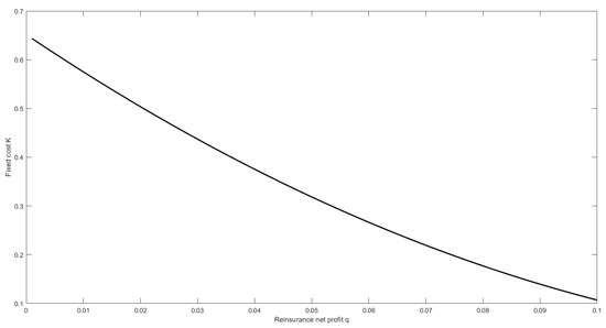
Figure 1. The effect of the reinsurer’s net profit q on $K^{*}$.

As illustrated in Figure 2, when the insurer is more risk averse, she is willing to pay a higher fixed cost. This result reinforces the practical implications of Equation (16), which implies that the more risk averse is the insurer, the larger protection she will buy.

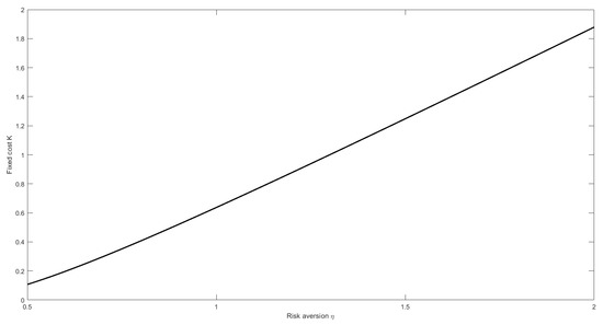
Figure 2. The effect of the risk-aversion parameter $\eta$ on $K^{*}$.

Figure 3 shows the effect of the potential losses. When they increase, that is ${\sigma }_0$ is high, then the insurer is going to pay high fixed cost in order to obtain protection.

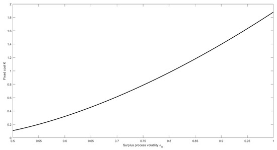
Figure 3. The effect of the volatility parameter $\sigma$ on $K^{*}$.

Finally, Figure 4 show that the larger the insurer’s time horizon is, the higher the fixed cost will be.

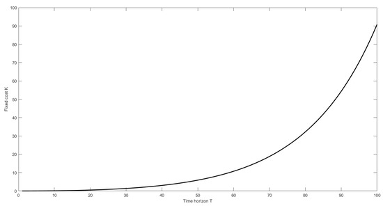
Figure 4. The effect of the time horizon T on $K^{*}$.

8. Conclusions

We investigate the optimal reinsurance problem under the assumption that a transaction cost is paid when the agreement is signed. The insurer has to choose the optimal starting time of the reinsurance contract, as well as the optimal retention level to be applied from that moment on. We solve the resulting mixed optimal control/optimal stopping time problem using a two-step procedure. We find that the optimal strategy is deterministic (see Theorem 4). Moreover, we prove the existence of a maximum fixed cost $K^{*}$ (see Equation (39)) that the insurer is willing to pay. That is, whenever a fixed cost $K>K^{*}$ is chosen by the reinsurer, the insurer will retain all her losses. In the last section, we further analyze how the model parameters affect that maximum subscription cost.

Some future research could be focused on the study of the optimal reinsurance problem with fixed cost under either different optimization criteria or different types of contract.

References

- De Finetti, B. Il problema dei “pieni”. G. Ist. Ital. Attuari 1940, 11, 1–88. [Google Scholar]
- Bühlmann, H. Mathematical Methods in Risk Theory; Springer: Berlin/Heidelberg, Germany, 1970. [Google Scholar]
- Gerber, H. Entscheidungskriterien für den zusammengesetzten Poisson-Prozess. Schweiz. Verein. Versicherungsmath. Mitt. 1969, 69, 185–228. [Google Scholar]
- Irgens, C.; Paulsen, J. Optimal control of risk exposure, reinsurance and investments for insurance portfolios. Insur. Math. Econ. 2004, 35, 21–51. [Google Scholar] [CrossRef]
- Brachetta, M.; Ceci, C. Optimal proportional reinsurance and investment for stochastic factor models. Insur. Math. Econ. 2019, 87, 15–33. [Google Scholar] [CrossRef]
- Brachetta, M.; Ceci, C. Optimal Excess-of-Loss Reinsurance for Stochastic Factor Risk Models. Risks 2019, 7, 48. [Google Scholar] [CrossRef]
- Skogh, G. The Transactions Cost Theory of Insurance: Contracting Impediments and Costs. J. Risk Insur. 1989, 56, 726–732. [Google Scholar] [CrossRef]
- Braouezec, Y. Public versus private insurance system with (and without) transaction costs: Optimal segmentation policy of an informed monopolist. Appl. Econ. 2019, 51, 1907–1928. [Google Scholar] [CrossRef]
- Egami, M.; Young, V.R. Optimal reinsurance strategy under fixed cost and delay. Stoch. Process. Their Appl. 2009, 119, 1015–1034. [Google Scholar] [CrossRef]
- Li, P.; Zhou, M.; Yin, C. Optimal reinsurance with both proportional and fixed costs. Stat. Probab. Lett. 2015, 106, 134–141. [Google Scholar] [CrossRef]
- Schmidli, H. Risk Theory; Springer Actuarial, Springer International Publishing: Berlin/Heidelberg, Germany, 2018. [Google Scholar]
- Karatzas, I.; Wang, H. Utility maximization with discretionary stopping. Siam J. Control. Optim. 2000, 39, 306–329. [Google Scholar] [CrossRef]
- Ceci, C.; Bassan, B. Mixed Optimal Stopping and Stochastic Control Problems with Semicontinuous Final Reward for Diffusion Processes. Stochastics Stoch. Rep. 2004, 76, 323–337. [Google Scholar] [CrossRef]
- Bouchard, B.; Touzi, N. Weak Dynamic Programming Principle for Viscosity Solutions. Siam J. Control. Optim. 2011, 49, 948–962. [Google Scholar] [CrossRef]
- Chen, M.; Yuen, K.C.; Wang, W. Optimal reinsurance and dividends with transaction costs and taxes under thinning structure. Scand. Actuar. J. 2020, 1–20. [Google Scholar] [CrossRef]
- Grandell, J. Aspects of Risk Theory; Springer: Berlin/Heidelberg, Germany, 1991. [Google Scholar]
- Eisenberg, J.; Schmidli, H. Optimal control of capital injections by reinsurance in a diffusion approximation. Blätter DGVFM 2009, 30, 1–13. [Google Scholar] [CrossRef]
- ∅ksendal, B. Stochastic Differential Equations; Springer: Berlin/Heidelberg, Germany, 2003. [Google Scholar]
Publisher’s Note: MDPI stays neutral with regard to jurisdictional claims in published maps and institutional affiliations. |
© 2021 by the authors. Licensee MDPI, Basel, Switzerland. This article is an open access article distributed under the terms and conditions of the Creative Commons Attribution (CC BY) license (http://creativecommons.org/licenses/by/4.0/).