Abstract
We show that interactions of inherently chaotic oscillators can lead to coexistence of regular oscillatory regimes and chaotic oscillations in the rings of coupled oscillators provided that the level of interaction between the oscillators exceeds a threshold value. The transformation of the initially chaotic dynamics into the regular dynamics in a number of the coupled oscillators is shown to result from suppression of chaos by separation of certain oscillation periods from the continuous spectra, which are characteristic of chaotic oscillations.
1. Introduction
Populations often demonstrate oscillatory dynamics [1]. These oscillations arise as a result of interactions between populations [2] and/or impacts of environmental factors, such as temperature, nutrient variations, and some others [3]. The role of a specific driving force in the emergence of oscillatory dynamics can be understood with the use of suitable mathematical models. For example, mathematical models have been widely used to study the mechanisms underlying chaotic variations in population size [4]. In particular, the models have been proved to be useful in assessing the impact of environmental heterogeneity on the horizon of predictability of chaotic plankton dynamics [5].
The results of mathematical modeling can be naturally supplemented and verified with the data obtained in the course of ecological monitoring. For example, the data obtained in the course of long-term monitoring of the ecosystem of the Naroch Lakes (Belarus) were used in order to analyze characteristics of hydrobiont population dynamics. As a result, it was shown that chaotic regimes, which often occur in mathematical models of aquatic ecosystems [3], are indeed characteristic of fluctuations in the plankton abundance in the Naroch Lakes [6]. Note that each of the relatively shallow lakes that constitute the Naroch lake ecosystem (oligo-mesotrophic Lake Naroch, mesotrophic Lake Myastro, and eutrophic Lake Batorino) is characterized by intensive mixing of water resulting in equalization the living conditions within each of these lakes [7]. Therefore, one could expect that the chaotic nature of the plankton abundance fluctuations detected by measurements at several points (lake monitoring stations) reflects the nature of plankton dynamics in the entire water body. Nevertheless, the question of whether this expectation is justified has so far remained unanswered.
In a more general form, this question can be reformulated as follows (regardless of any ecosystem): How stable is the dynamics of interconnected chaotic oscillators under a small local perturbation? We show here that interactions between inherently chaotic oscillators can lead to emergence of coexisting chaotic and regular oscillations.
2. Models
We analyze the dynamical modes, which arise in the chains of N coupled oscillators. The corresponding model is as follows:
where i is the number of the oscillator in the chain, t is time, and C is a constant. The first term on the right-hand side of Equation (1) represents the exchange processes between neighboring oscillators with periodic boundary conditions. The structure of the model of the coupled oscillators is shown in Figure 1. The periodicity of boundary conditions in this mathematical model reproduces the ring-like nature of real ecosystems (for example, coastal zones of closed reservoirs: ponds and lakes). The function in (2) represents the local dynamics, which is described either by the logistic map that was popularized by May [8], or as the Gompertz map [9].
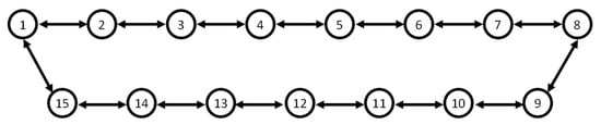
Figure 1.
Structure of the ring of oscillators.
For the logistic map
r is a constant. The logistic maps have been widely used in mathematical models of population dynamics [2].
The Gompertz function
where r is a constant, was originally put forward to describe human mortality in the assumption that a person’s resistance to death decreases exponentially as his/her years increase. Besides, the Gompertz function appears in fisheries ecology [10]. Under (i.e., for isolated oscillators), both the logistic map and Gompertz map have been shown to give rise to regular as well as to chaotic dynamics [2].
The ring of oscillators, which is described by (1) and (2), is assumed to consist of initially (at ) chaotic oscillators. Segments of the corresponding chaotic time series are shown in Figure 2a,c. The power spectra of these time series are shown in Figure 2b (the logistic map) and Figure 2d (the Gompertz map). One can see that the power spectra consist of peaks that are closely adjacent to each other. Such a structure of these spectra is a sign of chaos and makes it possible to distinguish the spectra of chaotic time series from those of periodic time series; the latter are composed from distinct separate peaks [11].

Figure 2.
Segments (250 time steps) of the chaotic time series (a,c), and the corresponding power spectra (b,d); the logistic map (a,b), ; the Gompertz map (c,d), . The values of the dominant Lyapunov exponent () are equal to +0.45 (a), and +0.43 (b). The positive Lyapunov exponents are a hallmark of chaotic dynamics [12].

The exchange processes arise when a small instantaneous perturbation () is introduced into the dynamics of one of the oscillators. In our case, .
3. Results
3.1. Coexisting Chaotic and Regular Dynamical Patterns in the Rings of Oscillators
Figure 3 demonstrates the dynamics of coupled logistic oscillators after the perturbation is applied. A result of the perturbation in the ring of coupled Gompertz oscillators is shown in Figure 4.
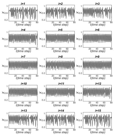
Figure 3.
Segments (80 time steps) of the logistic time series () that are the result of the perturbation after the completion of transients. This perturbation was applied to the 8-th oscillator () at . Here, .
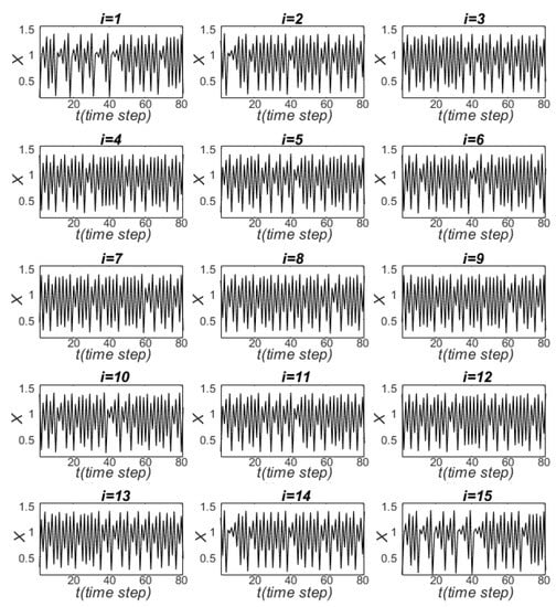
Figure 4.
Segments (80 time steps) of the Gompertz time series (), that are the result of the perturbation , after the completion of transients. This perturbation was applied to the 8-th oscillator () at t = 1001. Here, .
As it is seen from Figure 3 and Figure 4, the perturbation results in a violation of the initial identity of the oscillators. It is also seen that the oscillations for are identical to those for , the oscillations for are identical to those for , etc. This symmetry results from the choice of the perturbed oscillator location and the periodic boundary conditions. All the time series in Figure 3 and Figure 4 are chaotic (just as they were for , see Figure 2); the corresponding numerical values of the dominant Lyapunov exponent of the oscillations, which are shown in Figure 3 and Figure 4, range from +0.07 to +0.45 (the logistic map) and from +0.10 to +0.40 (the Gompertz map).
An increase in the intensity of the exchange processes between the oscillators causes a dramatic change in the character of their dynamics. In this case, despite the fact that some of the oscillators remain chaotic, others begin to oscillate in a regular manner. The domains of chaos coexisting with domains of regular dynamics occur both in the ring of logistic oscillators (Figure 5) and in the ring of oscillators whose activity is given by the Gompertz function (Figure 6). In Figure 5 and Figure 6, like in Figure 3 and Figure 4, the time series for are identical to those for , the time series for are identical to those for , etc.
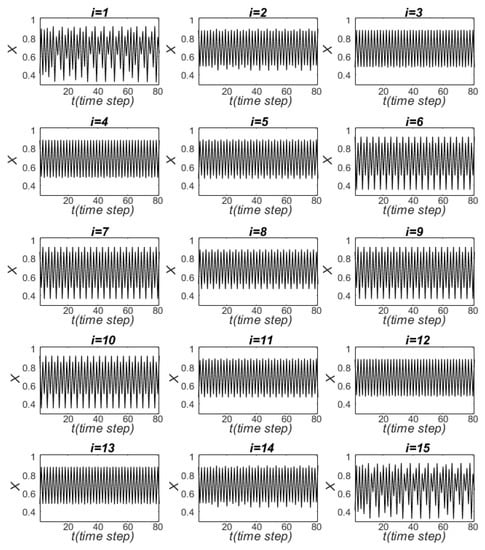
Figure 5.
Segments (80 time steps) of the logistic time series () that are the result of the perturbation after the completion of transients. This perturbation was applied to the 8-th oscillator () at . Here, .
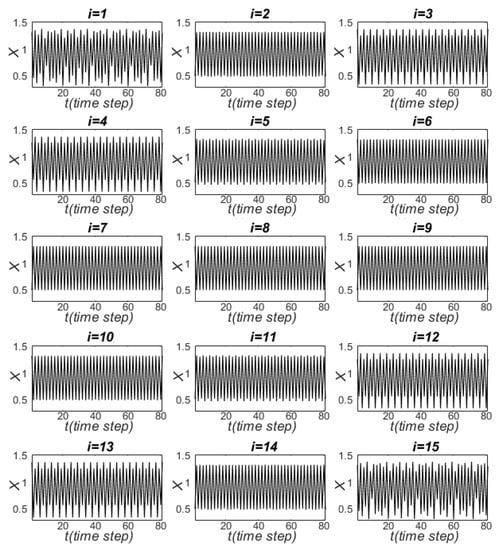
Figure 6.
Segments (80 time steps) of the Gompertz time series () that are the result of the perturbation after the completion of transients. This perturbation was applied to the 8-th oscillator () at . Here, .
For the chaotic time series shown in Figure 5 and Figure 6, both maximum and minimum numerical values of the dominant Lyapunov exponent are lower than the maximum and minimum values of characteristic of the chaotic time series under lower intensities of the exchange processes (Figure 3 and Figure 4). Namely, in contrast to the values of () characteristic of the time series for (Figure 3) for the ring of logistic oscillators and the values of (), which are characteristic of the time series for (Figure 4) for the Gompertz oscillators, the values of the chaotic time series in Figure 5 and Figure 6 are for , for , for (logistic oscillators), and for , for (Gompertz oscillators).
In more detail, the dynamical regimes that emerge in the ring of oscillators under variations in numerical values of the parameters r and C are shown in Figure 7.
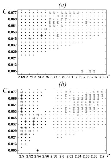
Figure 7.
The dynamical modes in the model parameter space (): (a) logistic oscillators, (b) Gompertz oscillators. Here, dots (·) denote the coexisting dynamical modes: chaos + regular oscillations, (⊙) corresponds to regular oscillations (chaotic modes do not occur in the ring), white color corresponds to chaotic modes of each of the oscillators of the ring.
One can see (Figure 7) that a slight increase in the parameter C values can lead to transition from chaotic dynamical regimes to coexistence of chaos and regular oscillations, or to regular oscillations, when chaos does not occur in the ring. Variations in the parameter r values can also lead to transitions from one dynamical regime to another.
3.2. Resonance as the Cause of Transformation of Chaos into Regular Dynamics
The phenomenon of coexistence of different dynamical regimes resulting from the transformation of the initial chaos into regular dynamics in a number of oscillators, while other oscillators in the same ring remain chaotic, turned out to depend on the intensity of the exchange processes between neighboring oscillators. However, the effect of the exchange processes on the dynamics of coupled neighboring oscillators is reduced to zero when these oscillators remain synchronized. This is the case for oscillations for and ().
Figure 8 demonstrates the power spectra of the logistic time series for , and 4, and the corresponding power spectra resulting from the exchange processes (). Oscillations for are chaotic, while regular behavior takes place for (Figure 5).
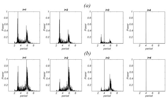
Figure 8.
(a) Power spectra of the logistic time series for , and 4, and (b) the power spectra of the corresponding exchange processes (). The power spectra were obtained for the time series on the interval [37953, 40000], when transients were completed.
Note the difference between the spectra of chaotic oscillations for in Figure 8a and the power spectra of the solitary chaotic oscillator (Figure 2a). One can see (Figure 8a) that the additional peak, which corresponds to the period , appears. Note that this peak also appears in the spectra of exchange processes (Figure 8b). The peak at is seen for . The value is also the period of both regular oscillations and the corresponding exchange processes (Figure 8a,b; ). Periodicity of other regular oscillators in the ring (Figure 5) is characterized by the same value .
The power spectra of both the Gompertz oscillators and the corresponding exchange processes () are shown in Figure 9. Here, in contrast to the logistic oscillators, the period appears even for (cf. Figure 8). Like in Figure 8 (for ), the value is the period of regular Gompertz oscillator (for ) and of the corresponding exchange processes (Figure 9a,b). Periodicity of other regular Gompertz oscillators is characterized by the same value .
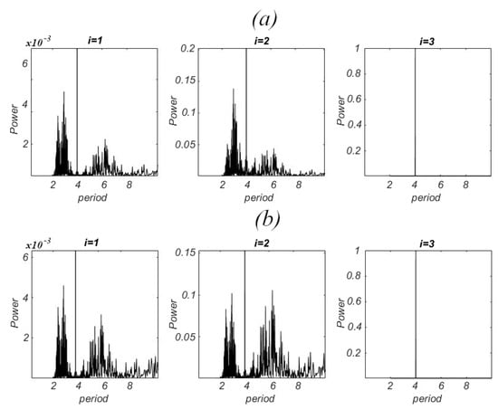
Figure 9.
(a) Power spectra of the Gompertz oscillators for , and 4, and (b) the power spectra of the corresponding oscillatory exchange processes (). The power spectra were obtained for the time series on the interval [37953, 40000], when transients were completed.
Figure 8 and Figure 9 demonstrate a similarity of the spectra of the time series of the logistic (3) and Gompertz (4) maps with the spectra of the corresponding exchange processes. Such a similarity implies that the dynamics of each of the coupled oscillators is essentially dependent on the exchange processes, and vice versa. At a sufficiently high intensity of the exchange processes, the resonance, i.e., the coincidence of one of the components of the spectrum of the exchange processes with a component of initially chaotic oscillations, causes the selection of the corresponding period of oscillations from the continuous spectrum characteristic of chaos. As a result, the chaotic dynamics is transformed into a regular one.
4. Concluding Remarks
Since the pioneering experiments by Galileo Galilei [13] (see also in [14]) and Christiaan Huygens [15] (see also in [16]), mechanisms of oscillatory processes and the effects associated with interactions between oscillatory processes have attracted the attention of researchers in various fields of physics, chemistry, biology, and ecology [3,17,18,19,20,21,22]. The interactions between individual oscillators, which result in a transformation of hardly predictable chaotic dynamics into regular dynamics, were of particular interest. In this context, it was shown, for example, that even a small feedback action can turn chaotic dynamics into periodic one, and vice versa [23]. Stable periodicity was demonstrated to arise when a chaotic system is driven by another chaotic system. This effect occurs to be a result of closeness of the chaotic dynamics of the response system to a periodic window [24]. As applied to ecological systems, it has been shown theoretically that coupling between two habitats can cause chaotic populations to behave non-chaotically [25,26,27].
We show here (Figure 5 and Figure 6) that coexistence of regular and chaotic oscillators can emerge in a ring of coupled oscillators. Self-organization of the domains, one of which includes regular oscillators, while the other consists of chaotic oscillators, occurs as a result of a small perturbation, which was applied to one of initially identical chaotic oscillators, followed by the selection of a component from the continuous spectrum typical of chaos (Figure 8 and Figure 9).
The ring of coupled oscillators can be considered as a complete dynamical system. This dynamical system can serve as a model of real ring-shaped ecosystems (for example, a near-shore area of a lake).
We use the Shannon entropy
as a numerical characteristic of the behavior of such a dynamical system. Here, t is time, and is the probability of the occurrence of the values (see Equation (1)) within the m-th interval of width :
Here, is a histogram, which displays the number of occurrences of the values within the m-th interval, and K is equal to the product of the number (N) of oscillators in the ring and the number of the random initial conditions set for calculating . The graphs for the rings of the oscillators, which are described by Equations (1)–(4), are shown in Figure 10.
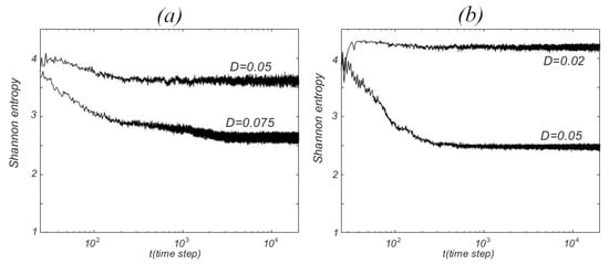
Figure 10.
The graphs obtained for random initial conditions: (a) the logistic map; (b) the Gompertz map. Here ; for the logistic map, and for the Gompertz map.
One can see that if the dynamics of all the oscillators in the ring remains chaotic over time (as for for the Gompertz map and for for the logistic map), then depends on time only weakly. A much more noticeable drop in the entropy (Figure 10; for the Gompertz map and for for the logistic map) occurs if, over time, the chaotic dynamics of most of the oscillators is transformed into regular dynamics (Figure 5 and Figure 6; see also the power spectra in Figure 8 and Figure 9). Thus, a shift in the value of the Shannon entropy over time may reflect the occurrence of qualitative changes in the dynamics of the system of coupled oscillators as a whole.
Note that the Gompertz map and the logistic map, as well as many other models that are employed in mathematical ecology [2], are essentially the product of a reduction-based approach. This means that any model is a simplification of reality, which is aimed at formalizing and analyzing the hypothesis concerning the mechanism of the phenomenon under study. Certainly, mathematical models are based on the data obtained from experiments and/or observations. However, even the planning of these experiments and observations presupposes selectivity and, consequently, a reduction of reality.
As an alternative to mathematical modeling, it was proposed to use reconstruction of population dynamics based on time series obtained from field observations in order to study the nature of population dynamics and predict the dynamics of population abundance [28]. On the other hand, in order to overcome the curse of reductionism [29], an approach called “hybrid modeling of population dynamics” has been proposed [30]. This approach involves direct incorporation of time series obtained by monitoring of natural ecosystems into the mathematical models. As a result, we get a chance to assess numerically the parameters of population dynamics that are difficult or even impossible to measure directly during field observations or experiments.
Both reconstruction of population dynamics and direct incorporation of the time series into mathematical models imply extensive and long-term field monitoring. Careful monitoring of natural ecosystems is equally necessary to assess whether chaotic and regular oscillations in population abundance can coexist even in a relatively homogeneous environment (for example, in shallow lakes, which are highly susceptible to wind mixing).
Author Contributions
Conceptualization, A.V.R. and A.B.M., methodology, A.V.R., D.A.T., N.I.N. and A.B.M., software and visualization, A.V.R., D.A.T. and N.I.N., investigation, interpretation and writing, A.V.R., D.A.T., N.I.N. and A.B.M. All authors have read and agreed to the published version of the manuscript.
Funding
The reported study was funded by the Institute of Theoretical and Experimental Biophysics of the Russian Academy of Sciences (state assignment 075-00381-21-00) and by the Institute of Mathematical Problems of Biology, Keldysh Institute of Applied Mathematics of the Russian Academy of Sciences (state assignment 0017-2019-0009).
Institutional Review Board Statement
Not applicable.
Informed Consent Statement
Not applicable.
Data Availability Statement
Not applicable.
Acknowledgments
We thank V.M. Tereshko for useful discussions. We are grateful to the reviewers for those comments that helped us prepare the updated version of the paper.
Conflicts of Interest
The authors declare no conflict of interest.
References
- Turchin, P. Complex Population Dynamics. A Theoretical/Empirical Synthesis; University Princeton: Oxford, UK, 2003; 452p. [Google Scholar]
- Kot, M. Elements of Mathematical Ecology; Cambridge University: Cambridge, UK, 2001; 464p. [Google Scholar]
- Solé, R.V.; Bascompte, J. Self-Organization in Complex Ecosystems; Princeton University: Princeton, NJ, USA, 2006; 372p. [Google Scholar]
- Otto, S.P.; Day, T. A Biologist’s Guide to Mathematical Modeling in Ecology and Evolution; Princeton University: Princeton, NJ, USA, 2007; 732p. [Google Scholar]
- Medvinsky, A.B. Chaos and predictability in population dynamics. Nonlinear Dyn. Psychol. Life Sci. 2009, 13, 311–326. [Google Scholar]
- Medvinsky, A.B.; Adamovich, B.V.; Chakraborty, A.; Lukyanova, E.V.; Mikheyeva, T.M.; Nurieva, N.I.; Radchikova, N.P.; Rusakov, A.V.; Zhukova, T.V. Chaos far away from the edge of chaos: A recurrence quantification analysis of plankton time series. Ecol. Complex. 2015, 23, 61–67. [Google Scholar] [CrossRef]
- Medvinsky, A.B.; Adamovich, B.V.; Aliev, R.R.; Chakraborty, A.; Lukyanova, E.V.; Mikheyeva, T.M.; Nikitina, L.V.; Nurieva, N.I.; Rusakov, A.V.; Zhukova, T.V. Temperature as a factor affecting fluctuations and predictability of the abundance of lake bacterioplankton. Ecol. Complex. 2017, 32, 90–98. [Google Scholar] [CrossRef]
- May, R.M. Biological populations with non-overlapping generations: Stable points, stable cycles, and chaos. Science 1974, 13, 311–326. [Google Scholar]
- Gompertz, B. On the nature of the function expressive of the low of mortality, and on a new method of determining the value of life contingencies. Philos. Trans. R. Soc. 1825, 27, 513–585. [Google Scholar]
- Fox, W.W. An exponential surplus yield model for optimizing in exploited fish populations. Trans. Am. Fish. Soc. 1970, 99, 80–88. [Google Scholar] [CrossRef]
- Kulp, C.W.; Niskala, B.J. Characterization of time series data. In Handbook of Applications of Chaos Theory; Skiadas, C.H., Skiadas, C., Eds.; CRC: Boca Raton, FL, USA, 2016; pp. 211–230. [Google Scholar]
- Boccara, N. Modeling Complex Systems; Springer: New York, NY, USA, 2004; 410p. [Google Scholar]
- Galilei, G. Discorsi e Dimostrazioni Matematiche, Intorno à due Nuoue Scienze; Ludovico Elseviro: Leida, Spain, 1638; 225p. [Google Scholar]
- Seeger, R.J. Galileo Galilei. His Life and His Works; Pergamon: New York, NY, USA, 1966; 286p. [Google Scholar]
- Huygens, C. Horologium Oscillatorium; Apud F. Muguet: Parisiis, France, 1673; 161p. [Google Scholar]
- Pikovsky, A.; Rosenblum, M.; Kurths, J. Synchronization. In A Universal Concept in Nonlinear Sciences; Cambridge University: Cambridge, UK, 2001; 433p. [Google Scholar]
- Kuramoto, Y. Chemical Oscillations, Waves and Turbulence; Springer: Berlin, Germany, 1984; 164p. [Google Scholar]
- Butylkin, V.S.; Kaplan, A.E.; Khronopulo, Y.G.; Yakubovich, E.I. Resonant Nonlinear Interactions of Light with Matter; Springer: Berlin/Heidelberg, Germany, 1989; 342p. [Google Scholar]
- Hanski, I. Metapopulation Ecology; Oxford University: New York, NY, USA, 1999; 324p. [Google Scholar]
- Freund, J.A.; Pöschel, T. (Eds.) Stochastic Processes in Physics, Chemistry, and Biology; Springer: Berlin/Heidelberg, Germany, 2000; 518p. [Google Scholar]
- Glass, L. Synchronization and rhythmic processes in physiology. Nature 2001, 410, 277–284. [Google Scholar] [CrossRef] [PubMed]
- Lawson, H.S.; Holló, G.; Horvath, R.; Kitahata, H.; Lagzi, I. Chemical resonance, beats, and frequency locking in forced chemical oscillatory systems. J. Phys. Chem. Lett. 2020, 11, 3014–3019. [Google Scholar] [CrossRef] [PubMed]
- Ott, E. Chaos in Dynamical Systems; Cambridge University: Cambridge, UK, 2002; 492p. [Google Scholar]
- Pisarchik, A.N.; Bashkirtseva, I.; Ryashko, L. Chaos can imply periodicity in coupled oscillators. Europhys. Lett. 2017, 117, 40005–40012. [Google Scholar] [CrossRef]
- Hastings, A. Complex interactions between dispersal and dynamics: Lessons from coupled logistic equations. Ecology 1993, 74, 1362–1372. [Google Scholar] [CrossRef]
- Vandermeer, J.; Kaufmann, A. Models of coupled population oscillators using 1-D maps. J. Math. Biol. 1998, 37, 178–202. [Google Scholar] [CrossRef][Green Version]
- Medvinsky, A.B.; Bobyrev, A.E.; Burmensky, V.A.; Kriksunov, E.A.; Nurieva, N.I.; Rusakov, A.V. Modeling aquatic communities: Trophic interactions and the body mass-and-age structure of fish populations give rise to long-period variations in fish population size. Russ. J. Numer. Anal. Math. Model. 2015, 30, 55–70. [Google Scholar] [CrossRef]
- Perretti, C.T.; Munch, S.B.; Sugihara, G. Model-free forecasting outperforms the correct mechanistic model for simulated and experimental data. Proc. Natl. Acad. Sci. USA 2013, 110, 5253–5257. [Google Scholar] [CrossRef] [PubMed]
- Viceconti, M. Multiscale modeling of human pathophysiology. In Biomechanics; Doblaré, M., Merodio, J., Eds.; Eolss Publishers: Singapore, 2015; pp. 413–435. [Google Scholar]
- Medvinsky, A.B.; Adamovich, B.V.; Rusakov, A.V.; Tikhonov, D.A.; Nurieva, N.I.; Tereshko, V.M. Population dynamics: Mathematical modeling and reality. Biophysics 2019, 64, 956–977. [Google Scholar] [CrossRef]


Publisher’s Note: MDPI stays neutral with regard to jurisdictional claims in published maps and institutional affiliations. |
© 2021 by the authors. Licensee MDPI, Basel, Switzerland. This article is an open access article distributed under the terms and conditions of the Creative Commons Attribution (CC BY) license (http://creativecommons.org/licenses/by/4.0/).