Combining Grammatical Evolution with Modal Interval Analysis: An Application to Solve Problems with Uncertainty

Abstract

Complex systems are usually affected by various sources of uncertainty, and it is essential to account for mechanisms that ensure the proper management of such disturbances. This paper introduces a novel approach to solve symbolic regression problems, which combines the potential of Grammatical Evolution to obtain solutions by describing the search space with context-free grammars, and the ability of Modal Interval Analysis (MIA) to handle quantified uncertainty. The presented methodology uses an MIA solver to evaluate the fitness function, which represents a novel method to manage uncertainty by means of interval-based prediction models. This paper first introduces the theory that establishes the basis of the proposed methodology, and follows with a description of the system architecture and implementation details. Then, we present an illustrative application example which consists of determining the outer and inner approximations of the mean velocity of the water current of a river stretch. Finally, the interpretation of the obtained results and the limitations of the proposed methodology are discussed.

1. Introduction

Continuous improvements in algorithmic problem-solving, together with an increase in the availability of high-performance computing, have resulted in a new generation of precise and highly detailed mathematical models [1]. The modeling of the physical properties within these systems is complex, because they are generally unknown or indeterminate. Explicitly incorporating uncertainty in the predictions of a model from the beginning is vital. The identification and management of uncertainty is essential to manage the complexity that occurs in numerous engineering applications [2]. Methods that model these uncertainties seek to develop robust mechanisms designed to remain flexible and resilient to appropriately react to new situations.

In general, the uncertainty of a system can arise from many sources, such as disturbances from the physical environment (e.g., variability in the flow controlling a water level), noise from devices that collect data (e.g., blood glucose readings from a continuous blood glucose monitor [3]), the representation of errors in physical quantities (e.g., the error in the gravitational acceleration constant $g=9.807\pm$ 0.027 m/s${}^2$), truncation errors in floating point operations, etc. These uncertainties will lead to undesired system behaviors if not addressed properly. Therefore, methodologies able to manage such uncertainty in a robust manner are required.

The purpose of this paper is to present a computational framework for solving symbolic regression problems, which is able to cope with the uncertainty encountered in real-life problems, and to make predictions accounting for such uncertainty. The proposed approach is based on interval analysis and data-driven optimization techniques. In particular, it combines the advantages of a grammar-based search algorithm [4] with the arithmetic of Modal Interval Analysis (MIA) [5]. The excellent flexibility of Grammatical Evolution (GE) for generating models, together with the inherent ability of MIA to manage uncertainty, led us to propose the development of a combined method to deal with the generation of predictive models from imprecise, or uncertain, data, without losing interpretability in the results. This study contributes to the literature by providing an evolutionary algorithm capable of working directly with MIA, which provides a mathematical framework to deal with quantified uncertainty. While the GE algorithm delimits the space of the solutions and guides the search, MIA manages uncertainty naturally and provides semantics to transform logical formulas into inclusion relationships, which are used to build the algorithm loss function. In order to illustrate the utilisation of the proposed approach, the resolution of a real-life problem, consisting of determining the meanstream velocity of the waters of a river stretch, is presented.

This paper is organized as follows. Uncertainty handling in predictive modeling is briefly reviewed in the next Subsection, while Section 2 and Section 3 summarize the foundations of GE and MIA theory, respectively. Section 4 introduces our proposed interval-based grammatical evolution approach. Section 5 presents an illustrative example, the required implementation steps, and the results. Finally, in Section 6, the obtained results are discussed and some conclusions provided.

Related Work

Two approaches are typically used to handle uncertainty in predictive modeling: explicit, or knowledge-driven, models and data-driven models. Techniques such as Bayesian networks, fuzzy logic, interval analysis, and rough sets have been successfully integrated into explicit, or knowledge-driven, models to address systems with uncertainty [6,7,8,9]. The advantage of these models is that they provide an explicit representation of the internal operation of the system to predict, simulate, and explain its behavior from the structure, causality, functional, and behavior of its components. However, these techniques are often computationally prohibitive or inaccurate for modelling complex systems that depend on a large number of variables. One of the more important techniques in this group is the well-know classical interval analysis. Classical intervals have shown a wide range of abilities, such as addressing problems using optimization to avoid overestimation of the optimal range of values [10,11,12]. In addition, the study of the solutions of a linear system when the coefficients and the independent term are considered as intervals has received much attention in the interval community, since it appears in the control design of different physical systems [13,14,15,16,17]. Pursuing the same line, in 2014 Modal Interval Analysis (MIA) [5], was presented as an extension of classical interval analysis. MIA allows uncertainty to be introduced, as classical intervals, in the generation of mathematical models by representing it using an interval (i.e., a pair of real numbers bounding a real domain). In addition to a range, model intervals are defined by a logical quantifier (∀ or ∃), that affects the represented uncertainty. Hence, MIA allows for a richer semantic interpretation of the results.

On the other hand, data-driven methods such as deep neural network techniques have focused on the extraction of predictive models from uncertain data [18]. Such models are especially effective when knowledge-driven models are difficult to build (e.g., owing to insufficient understanding of the underlying processes). Data-driven models cannot catch the physics of the modeled process; they just capture the relationships between the relevant input and output variables. However, such data-driven methods could potentially be more accurate than knowledge-driven models because they are based on objective information (i.e., data). The main drawback of all these black-box approaches is that they lead to a loss of result interpretability, and causality cannot be inferred. Machine-learning methods have been prompted by a recent wave of interest due to improvements in the algorithms (e.g., activation function) that have made such techniques more efficient. Finally, the combinations of more traditional approaches, such as control engineering theory, with artificial intelligence, have resulted in a number of hybrid approaches [19,20].

This paper introduces an approach to solve symbolic regression problems, combining the potential of MIA to handle uncertainties with the ability of GE to obtain solutions. MIA is a mature mathematical technique that has been widely applied in control engineering [21], modeling and simulation [22], civil engineering for structural control [23], biomedical applications [24], computer graphics [25], and finance for insurance problems [26]. On the other hand, GE is a relatively new machine-learning methodology with a modular architecture that is applied in the design and optimization of predictive models [27]. GE shows good performance in complex environments, such as financial forecasting [28] or blood glucose predictions [4].

To the best of our knowledge, evolutionary algorithms have not been previously used in combination with MIA and we have not found any work using interval methods combined with GE. However, different studies investigating hybrid methods applying interval analysis techniques to deal with uncertainties and evolutionary algorithms to guide the search of a solution have been proposed. For instance, hybrid approaches based on multi-objective evolutionary algorithms, either based on the conversion of an interval multi-objective evolutionary algorithm to a deterministic single- or multi-objective optimization problem [29,30,31], or based on the interval dominance relation [32,33]. Furthermore, hybrid approaches on multiple types of evolutionary algorithms have also been presented. For example, Sun et al. [34] implemented a particle swarm optimization method to power lithium-ion batteries, Femia et al. [35] applied a combination of affine arithmetic (an extension of interval arithmetic) and genetic algorithms for worst-case analysis in circuit tolerance analysis, while Claudio et al. presented an hybrid approach applying interval analysis in a cellular evolutionary strategy [36]. Finally, one of the closer studies we have found is the work performed by Keijer, which proposed to enhance genetic programming using interval arithmetic [37]. The author presented an approach to produce solutions which avoided undefined behaviours and which performed better than standard approaches.

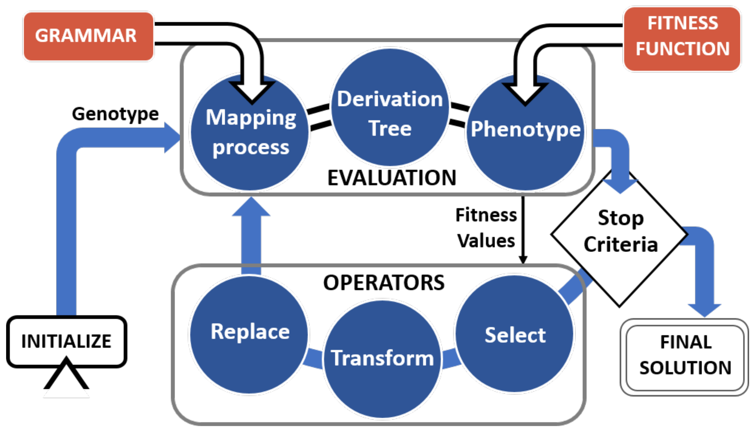
2. Predictive Modeling by Grammatical Evolution

One of the most compelling forms of evolutionary algorithms can be found in the GE methodology. GE is a search-based heuristic method with a modular design. It is widely used to solve optimization problems and is well-suited to the design of predictive models [27], which are, essentially, multivariate optimization problems. The goal of this search algorithm is to exploit historical information to guide it toward the regions of better performance within the search space. The general process of functioning in GE algorithms remains similar to those applied in other evolutionary algorithm approaches. Essentially, the algorithm initializes a population of solutions and initiates an iterative process that applies selection and transformation operators until the algorithm reaches an optimal solution or a predefined number of iterations.

The candidate solutions are presented as a sequence of codons. Typically, a codon comprises 8 bits representing an integer. Codons determine which specific grammar rules will be used.

The array of codons is called a genotype, while the code derived from the values is the phenotype. GE uses context-free grammar to enable a many-to-one mapping process, from genotypes to phenotypes. The genetic algorithm handles the generation of populations, whereas, at the phenotype level, solutions are evaluated in terms of a fitness function. Therefore, the genotype–phenotype mapping process involves the decoding of variable-length integer array (chromosomes) into expressions or programs in an arbitrary language. This feature allows the phenotype to be as complex as necessary, since all genetic operators are applied to the genotype. The general operation of the algorithm and the mapping process are outlined in Figure 1.

Context-Free Grammar

The key feature of predictive modeling via GE is the use of a context-free grammar (shortened to “grammar” hereinafter). This structure should incorporate knowledge related to the addressed problem. It comprises a set of rules that defines the structure of the generated candidate models. A grammar is defined by a 4-tuple $\{N,T,P,S\}$, where N and T are the set of non-terminal symbols and terminal symbols, respectively, P represents the production rules by which the symbols in N can be derived, and S the starting non-terminal symbol that must appear in N. The core of a grammar is typically defined in the Backus normal form (BNF)

$$\left[Symbol\right]\to productio{n}_1|...|productio{n}_k$$

(1)

Thus, given a grammar $G=\{N,T,P,S\}$, non-terminals N must be defined by a derivation rule, whereas terminals T are the lexicons of the predictive model language. The derivation rules in P comprise a non-terminal on the left-hand side $\left[Symbol\right]$ and its possible derivations on the right-hand side. Each rule definition comprises one or more alternatives separated by the symbol $“|”$. A single production is composed of a sequence $\sigma =({\sigma }_1,\cdots ,{\sigma }_n)$ where ${\sigma }_i\in N\cup T$ and $\#\sigma \ge 0$. Therefore, if we consider a production rule $\{\left[Symbo{l}_1\right]\to \gamma Symbo{l}_n\beta \}\in P$ where $\left[Symbo{l}_n\right]\in N$ and $\beta ,\gamma \in N\cup T$, we define that $\left[Symbo{l}_n\right]$ is a direct derivation of $\left[Symbo{l}_1\right]$, denoted as $\left[Symbo{l}_1\right]\Rightarrow \left[Symbo{l}_n\right]$, if a sequence of direct derivations exists

$$\begin{array}{ccc}& & \left[Symbo{l}_1\right]\Rightarrow \left[Symbo{l}_2\right],\hfill \\ & & \left[Symbo{l}_2\right]\Rightarrow \left[Symbo{l}_3\right],\hfill \\ & & \cdots ,\hfill \\ & & \left[Symbo{l}_{n-1}\right]\Rightarrow \left[Symbo{l}_n\right]\hfill \\ & & \mathrm{where}n\ge 0.\hfill \end{array}$$

(2)

A complete derivation tree is constructed by expanding all the non-terminals of the candidate solutions. Particularly, the process derives the leftmost non-terminal, as it is selected according the corresponding codon of the genotype. We repeat the process of derivation until the candidate solutions have no symbols remaining in N. During genotype mapping, we may reach the end of the genotype and be depleted of values before all non-terminals are transformed into terminals. At this point, the algorithm assesses the candidate model as an invalid solution. Therefore, candidate models are penalized if their genotypes lead to large phenotypes. Invalid solutions are assigned with poor fitness values, to discard in subsequent iterations.

3. Interval Methods

In interval analysis, a classical interval $[a,b]$ is defined as the set of numerical values x that lies between a and b, and operations are performed using intervals instead of real numbers.

$$[a,b]=\{x\in \mathbb{R}|a\le x\le b\}$$

(3)

In the system of intervals

$$I\left(\mathbb{R}\right)=\left\{\right[a,b\left]\right|a,b\in \mathbb{R},a\le b\}$$

(4)

the real arithmetic operators are introduced. An interval extension of a continuous function $z=f(x_1,...,x_n)$ from ${\mathbb{R}}^n$ to $\mathbb{R}$ is the interval united extension $R_f$ of f, defined as the domain of the f-values on its interval argument $X=(X_1,...,X_n)$ in $I\left({\mathbb{R}}^n\right)$

$$\begin{array}{ccc}& & R_f(X_1,\dots ,X_n)=\{z\mid x_1\in X_1,\dots ,x_n\in X_n\}=\hfill \\ & & {[min\{z\mid x_i\in X_i\},max\{z\mid x_i\in X_i\}]}_{i=1,\dots ,n}\hfill \end{array}$$

(5)

Because the interval united extension of a continuous function can not always be computed, an interval syntactic extension $fR(X_1,\dots ,X_n)$ is defined as its corresponding real function $f(x_1,\dots ,x_n)$ replacing their numerical arguments $x_1,\dots ,x_n$ by the interval arguments $X_1,\dots ,X_n$ and their “real” arithmetic operators by their corresponding interval operators, such that

$$R_f(X_1,\dots ,X_n)\subseteq fR(X_1,\dots ,X_n),$$

(6)

where $fR(X_1,\dots ,X_n)$, is computed from the bounds of the intervals $X_1,\dots ,X_n$. The interval syntactic extension is useful for computing the range of a function because it guarantees the result. However, the exact range is not obtained in the general case. This is because, in the case that a variable appears more than once in the expression of the function, each appearance is considered independent of the others, which leads to an overestimation of the real range.

3.1. Modal Interval Analysis

Modal interval analysis is a logical and algebraic completion of classical interval analysis, defined to overcome its semantic and algebraic deficiencies. The key concept is the inclusion of a logical quantifier in the definition of a modal interval. This provides semantic interpretation to the interval computations. For a more complete introduction to modal interval analysis, see [5,38].

A modal interval (see Figure 2), A, is a pair formed by a classic interval $A^{\prime }={[a,b]}^{\prime }$, its domain, and a logic quantifier ∀ or ∃, which is its modality, that is, $A=(A^{\prime },Q_A)$, where $Q_A$ is one of the logic quantifiers. Modal intervals of the type $A=(A^{\prime },\exists )$ are called proper intervals and modal intervals of the type $A=(A^{\prime },\forall )$ are called improper intervals. A set of modal intervals is denoted by $I^{*}\left(\mathbb{R}\right)$. A modal interval can be represented using its canonical coordinates in the form

$$A=[a,b]=\left\{\begin{array}{cc}({[a,b]}^{\prime },\exists )\hfill & \mathrm{if}a\le b\hfill \\ ({[b,a]}^{\prime },\forall )\hfill & \mathrm{if}a\ge b\hfill \end{array}\right.$$

(7)

For example, the interval $[1,3]$ is equal to $({[1,3]}^{\prime },\exists )$ and the interval $[3,1]$ is equal to $({[1,3]}^{\prime },\forall )$.

A convenient symmetry between proper and improper intervals is established by the duality operator, which changes the modality of a modal interval. Therefore, $\mathrm{Dual}\left(\right[a,b\left]\right)=[b,a]$.

The construction of modal intervals is completed with the concept of a modal quantifier Q defined by

$$Q(x,X)P\left(x\right)\iff \left\{\begin{array}{cc}(\exists x\in X^{\prime })P\left(x\right)\hfill & \mathrm{if}X=(X^{\prime },\exists )\hfill \\ (\forall x\in X^{\prime })P\left(x\right)\hfill & \mathrm{if}X=(X^{\prime },\forall )\hfill \end{array}\right.$$

(8)

that allows us to define the set of real predicates accepted as a modal interval $X=(X^{\prime },Q_X)$.

$$\mathrm{Pred}\left((X^{\prime },Q_X)\right):=\{P(.)\in \mathrm{Pred}\left(\mathbb{R}\right)\mid Q(x,(X^{\prime },Q_X))P\left(x\right)\}$$

(9)

The identification of a modal interval with the set of those real predicates that introduce the definition of the modal interval inclusion (see Figure 3). If $X,Y\in \mathrm{Pred}\left(\mathbb{R}\right)$,

$$X\subseteq Y\iff \mathrm{Pred}\left(X\right)\subseteq \mathrm{Pred}\left(Y\right)$$

(10)

Using their canonical coordinates, the inclusion between two modal intervals $A=[a_1,a_2]$ and $B=[b_1,b_2]$ is

$$\begin{array}{ccc}& & [a_1,a_2]\subseteq [b_1,b_2]\iff (a_1\ge b_1,a_2\le b_2)\hfill \\ & & [a_1,a_2]=[b_1,b_2]\iff (a_1=b_1,a_2=b_2)\hfill \end{array}$$

(11)

The lattice operations $meet$ and $join$ (see Figure 4) on $I^{*}\left(\mathbb{R}\right)$ for a bounded family of modal intervals $A\left(I\right):=\{A\left(i\right)=[a_1\left(i\right),a_2\left(i\right)]\in I^{*}\left(\mathbb{R}\right)\mid i\in I\}$ (I is the index’s domain) are defined as a function of the interval bounds as

$$\begin{array}{ccc}& & \left(meet\right){\wedge }_{i\in I}A\left(i\right)=[\underset{i\in I}{max}{a}_1\left(i\right),\underset{i\in I}{min}{a}_2\left(i\right)]\hfill \\ & & \left(join\right){\vee }_{i\in I}A\left(i\right)=[\underset{i\in I}{min}{a}_1\left(i\right),\underset{i\in I}{max}{a}_2\left(i\right)]\hfill \end{array}$$

(12)

The inequality relations (see Figure 5) lead to the lattice operators min and max. Consider a bounded family of modal intervals satisfying $A\left(J\right):=\{A\left(j\right)\in I^{*}\left(\mathbb{R}\right)\mid j\in J\}$. Hence, min and max are defined by the following equations

$$\begin{array}{c}\underset{j\in J}{min}A\left(j\right)=A\in I^{*}\left(\mathbb{R}\right)\mathrm{is}\mathrm{such}\mathrm{that}\hfill \\ (\forall j\in J)X\le A\left(j\right)\iff X\le A\hfill \end{array}$$

(13)

$$\begin{array}{c}\underset{j\in J}{max}A\left(j\right)=B\in I^{*}\left(\mathbb{R}\right)\mathrm{is}\mathrm{such}\mathrm{that}\hfill \\ (\forall j\in J)X\ge A\left(j\right)\iff X\ge B\hfill \end{array}$$

(14)

and computationally:

$$\begin{array}{ccc}& & \underset{j\in J}{min}A\left(j\right)=[\underset{j\in J}{min}{a}_1\left(j\right),\underset{j\in J}{min}{a}_2\left(j\right)].\hfill \end{array}$$

(15)

$$\begin{array}{ccc}& & \underset{j\in J}{max}A\left(i\right)=[\underset{j\in J}{max}{a}_1\left(j\right),\underset{j\in J}{max}{a}_2\left(j\right)].\hfill \end{array}$$

(16)

Important binary operators involving two operators, A and B, are the arithmetical operators $+,-,\ast ,/$, together with other operators, namely $log,exp,sin,\cdots$, and some metric operators, e.g., the width of an interval $A=[a_1,a_2]$, defined by $\mathrm{wid}\left(A\right)=a_2-a_1$, or distance, defined as

$$\mathrm{Tolerance}(A,B)=max\left\{\right|a_1-b_1|,|a_2-b_2\left|\right\},$$

which allows for the inclusion to be characterized by the 0 value.

$$\begin{array}{ccc}\hfill A\subseteq B\iff & & \mathrm{Tolerance}(A,A\wedge B)=0\mathrm{or}\hfill \\ & & \mathrm{Tolerance}(B,A\vee B)=0\hfill \end{array}$$

(17)

3.2. Modal Interval Extensions

Two modal interval extensions exist for a continuous function f from ${\mathbb{R}}^n$ to $\mathbb{R}$ in the variables $x=(x_1,\cdots ,x_n)$ to the n-dimensional interval $X=(X_1,\cdots ,X_n)$, and a split in its proper and improper interval components $X=(X_p,X_i)$,

$$\begin{array}{c}\hfill f^{*}\left(X\right)={\bigvee }_{x_p\in X_p^{\prime }}{\bigwedge }_{x_i\in X_i^{\prime }}[f(x_p,x_i),f(x_p,x_i)]=\\ \hfill =[\underset{x_p\in X_p^{\prime }}{min}\underset{x_i\in X_i^{\prime }}{max}f(x_p,x_i),\underset{x_p\in X_p^{\prime }}{max}\underset{x_i\in X_i^{\prime }}{min}f(x_p,x_i)].\end{array}$$

(18)

which is called the *-semantic extension of f, and the following, which is its **-semantic extension

$$\begin{array}{c}\hfill f^{**}\left(X\right):={\bigwedge }_{x_i\in X_i^{\prime }}{\bigvee }_{x_p\in X_p^{\prime }}[f(x_p,x_i),f(x_p,x_i)]=\\ \hfill =[\underset{x_i\in X_i^{\prime }}{max}\underset{x_p\in X_p^{\prime }}{min}f(x_p,x_i),\underset{x_i\in X_i^{\prime }}{min}\underset{x_p\in X_p^{\prime }}{max}f(x_p,x_i)].\end{array}$$

(19)

Both are related by the equality

$$f^{**}\left(X\right)=\mathrm{Dual}\left(f^{*}\left(\mathrm{Dual}\left(X\right)\right)\right)$$

(20)

3.3. Primary Theorems

The following two key results, named the * and ** semantic theorems, provide a logical interpretation to these semantic extensions.

*-semantic theorem: Given a continuous real function $f:{\mathbb{R}}^n\to \mathbb{R}$ and a modal vector $A\in I^{*}\left({\mathbb{R}}^n\right)$, whenever $F\left(A\right)\in I^{*}\left(\mathbb{R}\right)$ exists

$$\begin{array}{ccc}& & f^{*}\left(X\right)\subseteq F\left(A\right)\iff \hfill \\ & & (\forall a_p\in A_p^{\prime })(Qz\in F{\left(A\right)}^{\prime })(\exists a_i\in A_i^{\prime })\hfill \\ & & z=f(a_p,a_i).\hfill \end{array}$$

(21)

and **-semantic theorem: Given a continuous real function $f:{\mathbb{R}}^n\to \mathbb{R}$ and a modal vector $A\in I^{*}\left({\mathbb{R}}^n\right)$, whenever $F\left(A\right)\in I^{*}\left(\mathbb{R}\right)$ exists,

$$\begin{array}{ccc}& & f^{**}\left(X\right)\supseteq F\left(A\right)\iff \hfill \\ & & (\forall a_i\in A_i^{\prime })(Qz\in \mathrm{Dual}{\left(F\left(A\right)\right)}^{\prime })(\exists a_p\in A_p^{\prime })\hfill \\ & & z=f(a_p,a_i).\hfill \end{array}$$

(22)

For a given n-dimensional interval A, computing $f^{*}\left(A\right)$ (or $f^{**}\left(A\right)$) can be a difficult problem, except for simple cases. When the function f is a one- or two-variable operator, the computations are easy to obtain and, as for the arithmetic operators, the results are the same as the ones obtained via Kaucher arithmetic [39].

The values of semantic extensions, $f^{*}$ and $f^{**}$, can not be obtained by direct computation, except for simple real functions. If f is a ${\mathbb{R}}^n$ to $\mathbb{R}$ continuous with the syntactic tree function, its syntactic extension to the modal intervals $X_1,\cdots ,X_n$, is represented by $fR(X_1,\cdots ,X_n)$, is the function $fR$ from $I^{*}\left({\mathbb{R}}^n\right)$ to $I^{*}\left(\mathbb{R}\right)$ defined by the computational program indicated by the syntax tree of f. Modal syntactic functions are easy to compute but are generally not interpretable. To overcome this problem, semantic theorems provide inclusion relations to the corresponding *- and **-semantic extensions. Computations with $fR\left(X\right)$ must be performed with the external truncation of each operator to obtain the inclusions $f^{*}\left(X\right)\subseteq fR\left(X\right)$, and with the inner truncation to obtain the inclusions $fR\left(X\right)\subseteq f^{**}\left(X\right)$. In many cases, the rational extension $fR\left(X\right)$ is optimal, i.e.,

$$f^{*}\left(X\right)=fR\left(X\right)=f^{**}\left(X\right).$$

(23)

Modal interval analysis provides results for these inclusions or equalities. Coercion theorems provide the conditions and the method to obtain the optimal extensions according to the monotony.

3.4. $f^{*}$ Algorithm

When these theorems and their results are not applicable, the so-called $f^{*}$ algorithm, based on branch-and-bound techniques, yields the inner and outer approximations to $f^{*}$. Consider a continuous function $f(u,v)$, and its associated proper and improper interval vectors. $(U,V)$.

To obtain the inner (Inn) and the outer (Out) approximations of $f^{*}(U,V)$ or $f^{**}(U,V)$, we divide the initial domain into cells such that, in each of them, the monotony conditions necessary to apply the optimality theorems of modal interval analysis are met. The $f^{*}$ algorithm applies a set of strategies to minimize the number of bisections, and to obtain better local approximations of the resulting partitions. A tolerance function, defined as the distance between inner and outer approximation, provides the criteria to stop the algorithm

$$\begin{array}{ccc}\hfill & \mathrm{Tolerance}(\mathrm{Inn},\mathrm{Out})=\hfill & \hfill \\ \hfill & =max\left(\right|\mathrm{Inf}\left(\mathrm{Out}\right)-\mathrm{Inf}\left(\mathrm{Inn}\right)|,|\mathrm{Sup}\left(\mathrm{Out}\right)-\mathrm{Sup}\left(\mathrm{Inn}\right)\left|\right)\hfill \end{array}$$

(24)

where Inf and Sup are the left and right bounds of the corresponding approximations, respectively.

If we assume a desired tolerance $\phi$ for the output, the algorithm stops when $\mathrm{Tolerance}$$(\mathrm{Inn},\mathrm{Out})\le \phi$. The algorithm also stops when the width of all cell dimensions is smaller than a fixed precision $\left(\mathrm{wid}\right(X)\le ϵ)$. A standalone version of this algorithm can be found online, incorporated in the modal interval calculator package [40,41].

4. Interval-Based Grammatical Evolution

Evolutionary algorithms are are well-known because their high scalability and flexibility. They have been largely studied, and countless approaches can be found in the literature. There are other algorithms in this category, such as genetic algorithms and genetic programming, to name just two of the most popular members. The idea of an MIA-based extension of an evolutionary algorithm should be applicable in a more traditional setting than GE, such as in the aforementioned methodologies. GE has been chosen because of its versatility and adaptability to extract models from data and our experience working with it.

Figure 6 shows a schematic representation of the general architecture and the operation of the proposed methodology. Initially, the system is powered by a database (A) that provides the required information for system training and the subsequent validation of the method. In addition to the above-mentioned data sources, there are two other primary system inputs that must be defined according to the addressed problem. First, the definition of a problem-specific objective function (B), which evaluates the solutions. Secondly, a customized grammar (C), which defines the structure of the generated solutions. The module implementing the arithmetic of modal intervals is responsible for the interval operations associated with the solutions generated by the system (E). Solutions are iteratively combined to create new and better solutions, aiming to incrementally improve the quality of solutions (F) and reach a final solution that minimizes the fitness function satisfactorily. Once a final solution (G) is generated, the prediction model is evaluated using data from the remaining database information. The following subsections describe the complete setup of this methodology in detail.

4.1. Including Uncertainty in Grammatical Evolution

Given a set of the experimental measures y, we shall consider a predictive model defined by a continuous function f

$$\widehat{y}=f(y_0,p),$$

(25)

where $\widehat{y}$ is the state variable corresponding to y, $y_0$ the initial values, and p are the model parameters. If we assume uncertainty in the variables and the experimental measures of this model, we obtain the interval model defined by

$$\widehat{Y}=f^{*}(Y_0,P)\mathrm{or}\widehat{Y}=f^{**}(Y_0,P),$$

(26)

where P, $Y_0$ and, consequently, the model output ($\widehat{Y}$) are proper or improper intervals.

The generation of models that satisfy the aforementioned equation would require the implementation of mechanisms to achieve the following

• Manage intervals as inputs of the system;
• Generate intervals as parameters;
• Compute intervals as basic operations.

Therefore, the integration of uncertainty management into the method of GE directly affects its two essential features: the use of context-free grammar and the fitness function.

4.2. Uncertainty in Context-Free Grammars

First, before beginning the search-based process of GE (see Figure 1), the method incorporates a series of preprocessing mechanisms to enable intervals as a native data type in the computational framework. Interval inputs I associated with the explored methodology can be defined using the lower and upper bounds of the interval following Equation (3) or by defining an increment in the discrete values as follows

$$\begin{array}{c}\hfill I\left(\mathbb{R}\right)=\left\{\right[x\pm \Delta x\left]\right|x,\Delta x\in \mathbb{R}\}.\end{array}$$

(27)

Therefore, the method encompasses the typical cases and formats to gather data. Meanwhile, the data input may involve uncertain factors provided by the intervals; this is typical in cases where inaccuracy should be determined via repetitive trials, e.g., air-pollutant concentrations [42]. Nevertheless, the data entries may be defined as the imprecision of measuring devices; this is a typical and realistic scenario in which inaccuracy is associated to an error rate, e.g., in a continuous blood glucose monitor [3].

Additionally, the framework aimed to define the associated grammar that provides the possibility of generating interval parameters as an alternative to constant values. Thus, the predictive-modeling search engine can include intervals in the form $[x\pm \Delta x]$ into the candidate models. This feature is intended to represent the uncertainty of a parameter without an a priori associated error or deviation values, e.g., the circadian variability of a patient with diabetes [43].

4.3. Intervalized Fitness Functions

The role of the inclusion of uncertainty and the integration of intervals in the assessment criteria has important implications. Because the outcome of the candidate model evaluations implies an interval representation, two generic approaches are available to guide the definition of a fitness function. These can be defined depending on the inclusion relationship between the experimental data and the output of the model. If the pursued model requires the inclusion of the experimental data in the model estimates, then $\widehat{Y}=f^{**}(Y_0,P)\supseteq Y$ with, e.g., $Y_0$ and P as proper intervals. Therefore, we obtain the following expression by applying the **-semantic theorem

$$(\forall y\in Y^{\prime })(\exists y_0\in Y_0^{\prime })(\exists p\in P^{\prime })y=f(y_0,p).$$

(28)

According to (17), this inclusion is obtained by minimizing an assessment criterion

$$\mathrm{Tolerance}(Y,Y\wedge \widehat{Y})\mathrm{or}\mathrm{Tolerance}(\widehat{Y},Y\vee \widehat{Y})$$

(29)

Otherwise, if the requirement is that the estimated solutions are to be contained in the experimental dataset, i.e., $\widehat{Y}=f^{*}(Y_0,P)\subseteq Y$, we apply the *-semantic theorem to obtain

$$(\forall y_0\in Y_0^{\prime })(\forall p\in P^{\prime })(\exists y\in Y^{\prime })y=f(y_0,p).$$

(30)

Therefore, the evaluation criteria to be minimized in this case are

$$\mathrm{Tolerance}(\widehat{Y},Y\wedge \widehat{Y})\mathrm{or}\mathrm{Tolerance}(Y,Y\vee \widehat{Y})$$

(31)

These generic criteria might be sufficient to handle most predictive modeling problems. However, according to the semantic theorems and the inclusion conditions considered, new semantics can be proposed by varying the modalities of the associated intervals.

Finally, the proposed methodology supports the complete set of interval arithmetic operations, including the required $f^{*}$ algorithm, provided that multi-incidence is considered in the generation of the models. Both of them are presented in Section 3 and are essential for computing the final outcomes and training fitness values.

4.4. Predictive Modeling Solutions

GE is an evolutionary algorithm that mimics the natural selection process and, in this mimicked process, randomness is crucial. The stochastic nature of GE makes it a method well suited for problems with high requirements, but it should be remembered that GE is a probabilistic stochastic search algorithm, and solution models may vary across different executions. This method can assess a large number of candidate prediction models that iteratively converge to the final model. However, GE algorithms have not been proven to converge to the global optima of the fitness function in a finite time. Thus, an efficient evolutionary algorithm, which typically implies a balance of exploration and exploitation of the solutions, is usually expected to converge to multiple sub-optimal solutions rather than to the global optima. Different strategies can be implemented to select the sub-optimal prediction model that can be used to provide new estimations from unseen data inputs; however, they will not be discussed herein, as they are out of the scope of this study.

The proposed combination of interval methods and GE aims to obtain a soft interval band of estimated intervals that contains, is contained, or is simply the closest to the input intervals that are to be modeled. However, a discrete approximation, e.g., an independent modeling of the upper and lower boundaries of a set of intervals, would aim to obtain two trajectories that coincide or are close to the upper and lower boundary points, regardless of whether the other extreme coincides or is close to the other extreme of the interval. Thus, a non-interval approach could not generate a soft-band solution if the trajectories intersect. In addition, operating directly with intervals allows us to enter conditions and constraints in the form of logical conditions. By defining the semantics, the modal intervals allow us to transform these logical formulas into their equivalent form as inclusion relationships between the modal intervals. Therefore, the interval-based methodology presented herein is indispensable to generate solutions that follow such semantics.

5. Implementation, Results, and Discussions

5.1. Illustrative Example

In this section, we present an illustrative example in which interval GE is applied to the problem of determining the average water velocity of a river stretch. We used the interval GE methodology to build a model based on the bed slope and flow rate of the river. The method aims to capture the dynamics of the water velocity while managing the uncertainty associated to the physical system. Thus, the expected output of the model is the velocity of the river, whereas the model parameters are the river flow and the bed slope intervals. The interval model that we present in this section is presented as a mere example of the ability of the interval GE methodology to generate models from intervalized data.

The experimental dataset was obtained from a study aimed to generate a water-quality model of the Bajo Ter river (Spain) [44]. The measurements include the bed slope (m/m), the river flow rate (${\mathrm{m}}^3$/s), and the average surface velocity (m/s) of the river. To encompass a wide range of possible flow rates and a variety of bed slope values that could comprise the river’s extreme values, the measurements of the experimental values were performed at different locations along the river and at different times, and their values were modeled as intervals.

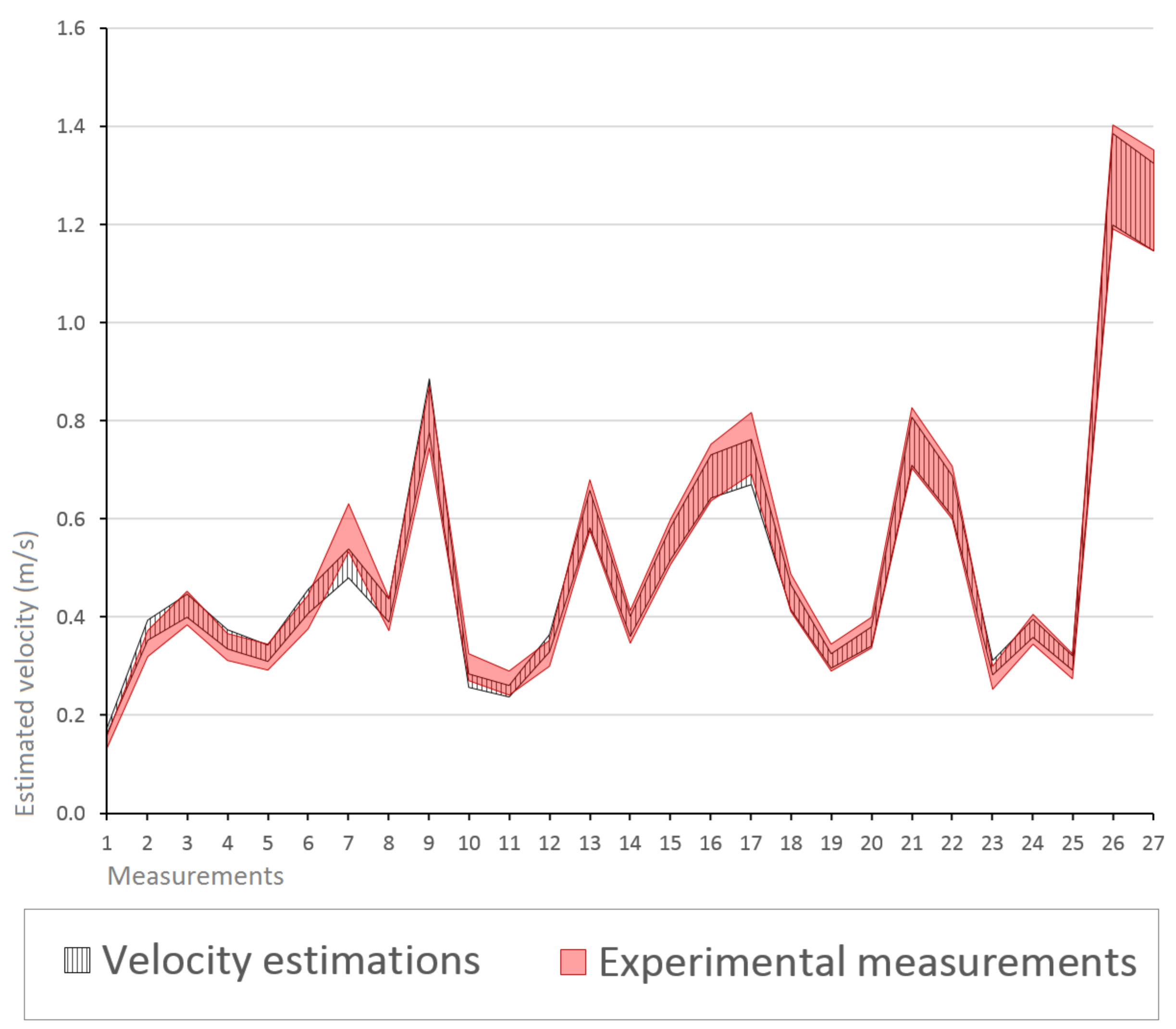
5.2. Modeling River Velocity

The grammar structure used in this case study is simple but flexible, and is adequate for illustrating the mechanism of the method. The grammar defined to estimate river velocity values is presented in Algorithm 1.

The non-terminal $\left[\lambda \right]$ is defined by a derivation rule, with no production involved. This non-terminal, aside from be a path to avoid the generation of any production of $\left[OperatorComplex\right]$, allows for the termination of the recursion originated by the production $\left[OperatorComplex\right]\left[OperatorComplex\right]$. The expressions generated by this grammar comprise a variable number of mathematical operations using the bed slope and flow-rate variables. In order to illustrate the modeling process, Equation (32) presents a basic example of a model solution derived from this grammar

$${\widehat{V}}_t=[0.4,0.6].\sqrt{B{s}_t^{1.1}}.\frac{0.11}{\left(F{r}_t^{1.9}\right)}+0.9.F{r}_t$$

(32)

where ${\widehat{V}}_t$ is the predicted velocity of the waters, $Bs$ is the bed slope and $Fr$ is the river flow rate for a given step t.

Algorithm 1: Context-free grammar used in our case study, where [Constant] is a non-terminal that generates real constants following a classical implementation via digit concatenation.

[Expression] →     [Term] | [Term][OperatorSimple][Expression]   [Term] →     ([Interval] [OperatorB] [OperatorComplex] (Bed Slope∧[Constant])) |     ([Interval] [OperatorB] [OperatorComplex] (Flow Rate∧[Constant]))   [OperatorComplex] →     sqrt | sin | log | pow | [Constant]∧ |     cos | [OperatorComplex][OperatorComplex] | [$\lambda$]   [OperatorSimple] →     [OperatorA] | [OperatorB]   [OperatorA] → + | -   [OperatorB] → * | ÷

The goodness of the achieved fit relies on the previous grammar definition, and also on the definition of a criterion to evaluate each model of the population. The definition of the fitness function guides the methodology toward an objective that will be used to model the final solutions. In this case study, we analyze different fitness functions based on the error calculation between the experimental measures and the estimated intervals. The goal is to achieve the most accurate approximation according to the experimental measurements. Here, we propose adjusting our estimates using two general approaches for an interval problem: an external and internal approximation to experimental values. First, we consider an external approximation of the estimates, i.e., we seek solutions that contain the experimental measures, thus fulfilling the following condition

$$V_i\subseteq \widehat{V_i}\iff \mathrm{Tolerance}(V_i,\widehat{V_i}\wedge V_i)=0.$$

(33)

Therefore, we define the first assessment criteria as the minimum distance between the experimental and estimated intervals constrained by condition (33)

$$C_1=\sum _i\mathrm{Tolerance}(\widehat{V_i},V_i)+K·\mathrm{Tolerance}(V_i,\widehat{V_i}\wedge V_i),$$

(34)

where K is a constant for weighting constraint (33).

Secondly, we consider an internal approximation of the estimates, i.e., we seek solutions that are contained in the experimental measures, thus fulfilling the following condition

$$\widehat{V_i}\subseteq V_i\iff \mathrm{Tolerance}(\widehat{V_i},\widehat{V_i}\wedge V_i)=0$$

(35)

Therefore, we define the first assessment criteria as the minimum distance between the experimental and estimated intervals constrained by condition (35)

$$C_2=\sum _i\mathrm{Tolerance}(\widehat{V_i},V_i)+K·\mathrm{Tolerance}(\widehat{V_i},\widehat{V_i}\wedge V_i),$$

(36)

where K is, once again, a constant for weighing the constraint.

The methodology adjusts the model parameters using previously collected historical data, i.e., the experimental measurements of the river. Additionally, the method has to be adjusted using a set of hyperparameters that express a higher level of structural settings and are not explicitly learned from the data.

Table 1. Hyperparameters of the GE implementation and its operators.

Hyperparameter	Value
Population size	500
Generations	100
Crossover prob.	0.9
Mutation prob.	0.03
K (weighting factor)	10
Tournament size	2
Max. Wraps	1
Chromosome length	50
Elitism	1
N (number of executions)	20

defines the values of these hyperparameters, which were selected empirically and are associated with the operators used in this implementation.

5.3. Results

The aim of this case study is to generate and evaluate the solutions for a modeling problem scenario that uses information contained in an experimental database. This section presents the estimated results of the two presented approaches and their assessment in terms of the typical performance metrics used to evaluate predictive accuracy.

The first step in analyzing this case study is to examine the convergence of the evolutionary algorithm. Figure 7 illustrates the average, maximum, and minimum fitness achieved from the best individuals of the proposed method using the assessment criteria $C_1$. The fitness value is represented with a logarithmic scale on the y-axis and the number of generations on the horizontal axis. Results show the mean values of the best individual, the fittest 50 individuals and the complete population. Similar to all the experiments presented in this study, performance was assessed after 20 runs, because the method is a probabilistic stochastic search algorithm.

Next, we evaluate the estimation results of the approach using the two previously defined assessment criteria. The results are presented in Figure 8 and Figure 9, which are a graphical representation of the outcomes and illustrate the differences between the internal and external approximations. They show the estimated average velocity values of the waters in the analyzed river stretch and the standard deviation ($\sigma$) of the computed intervals. The interval results are the mean average of 20 executions, and they estimate a range of possible values, thus including the uncertainty of the system in the estimations. Meanwhile, the standard deviation values indicate the variability of the set of executions in each of the interval bounds.

To evaluate the impact of interval operations on runtime, we implemented a version of the algorithm that does not use interval arithmetic in the assessment evaluations. This version is limited to training models that minimize the root–mean–square error (RMSE) of the mean value between the upper and lower limits of the experimental intervals. Figure 10 represents the mean times’ ± standard deviation of 20 trials. Considering that the variation in the computation time between $C_1$ and $C_2$ is negligible, we used condition $C_1$ for these trials.

5.4. Discussion

In this study, we presented an interval-based GE methodology, providing both its theoretical foundations and implementation details. We also introduced an innovative approach aiming to resolve regression problems affected by uncertainty. Finally, a series of experiments to test and illustrate the proposed method have been presented. Figure 7 shows how the functioning of the algorithm provides a population that is incrementally fitted through generations. The mean values of the best individuals achieve the best solution in the 80th generation, while the 50 fittest individuals give shape to a typical exponential function that converges at the mean minimum value at approximately the 100th generation. The curve representing all the individuals does not converge at the same values because the functioning of the crossover operator implements a measure to avoid premature convergence of the population. The operator avoids the generation of identical individuals in the same population by replacing these individuals with new randomized chromosomes. Therefore, there is a variable percentage of the population that is generated randomly each generation, and increments the mean value of fitness values.

As mentioned above, the objective is to analyze two complementary and general approaches for an interval problem, an external and an internal approximation with the targets $C_1$ and $C_2$, respectively. Although the defined criteria were not fulfilled in all the experimental points, the obtained intervals suggest a fitted representation of the models for both of them. The ${\widehat{V}}_{C1}:[a,b]$ provides mean standard deviation values of 0.017 and 0.018 and ${\widehat{V}}_{C2}:[c,d]$ mean standard deviation values of 0.002 and 0.001, which are satisfactorily low compared with our cost function, indicating a competitive design of the GE algorithm.

Figure 7 also shows how the evaluation times of both implementations decrease as the population converges, and that new assessments are not required. After comparing this with the version that does not use intervals, we observed a significant increase in the evaluation times, with an average multiplier of 3.7 over the version that does not use intervals.

The method is strongly influenced by the nature of the addressed problem; this implies a trade-off between the complexity of the solution-seeking space and the convergence of the algorithm. Moreover, it is not exempt from the typical drawbacks of evolutionary computation methods, such as the reproducibility of the results, the risk of premature convergence, and the high computational effort required. The latter is of significant importance, mainly due to the $f^{*}$ function evaluation, which leads to a significant increase in the computational power required by the system. This is especially due to the branch-and-bound nature of such algorithms, which aims to reduce the so-called interval overestimation problem. The use of the $f^{*}$ function involves an inherent algorithmic complexity that grows with the number of non-monotonic variables, the individuals, and the generations.

Typically, modern machine-learning techniques have a high computational costs due to the nature of the involved algorithms. An important example is deep-learning methods, which have recently attracted significant attention from the scientific community and industry, which are willing to invest in the required high-performance hardware systems. A serious drawback of GE is its inefficiency when implemented sequentially, as is the case here. However, GEs have inherent parallel properties that allow them to be successfully parallellized and obtain considerable accelerations (e.g., calculate the fitness of all chromosomes in the current population in parallel). The methodology presented herein still offers ample room for algorithm optimization and a parallelizable architecture, which could lead to a more mature and efficient machine-learning method.

The experiments conducted were performed based on an instance of a real case, which was presented as a practical approach to show the proposal. However, the real utility of the proposed method would be oriented to model more complex real-world problems from imprecise or uncertain data. A good example could be the glycemic monitoring of type 1 diabetics patients with continuous glucose sensors. The monitoring of blood glucose permits subjects detect unusual behavior of their glucose dynamics or even take preventive actions before the occurrence of an adverse events, reducing the risk of complications. Since continuous glucose monitoring devices were launched, the gathered historical data are used by data-driven models to capture the dynamics of blood glucose levels [20]; however, the measurement accuracy of these devices is far from optimal [45]. In addition to this lack of accuracy, we must add the delays that are intrinsically linked with the measurements on these devices [46,47]. Here, machine-learning methods could be applied to acquire and maintain knowledge based on treatment information; however, models will be always biased by the aforementioned measurement errors. This is an open problem in the diabetes technology community, and we hope to contribute to the solution by using the methodology presented in this paper.

6. Conclusions

Completely eliminating uncertainty from physical systems is often impossible; hence, a proactive approach to manage uncertainty is required. The presented approach acknowledges the existence of uncertainty and uses intervals to power a GE system architecture aiming to resolve regression problems. The methodology involves an evolutionary engine based on a GE approach that implements a set of features to operate with MIA. The context-free grammar itself allows for the attribution of knowledge that delimits the search space of the solutions, whereas the intervals allowed for the uncertainty to be managed naturally and MIA provide semantics that allows to transform logical formulas into inclusion relationships.

This work has explored the first evolutionary algorithm that enables interval arithmetic, thus handling uncertainties by a search algorithm. Furthermore, it has studied the role of uncertainty and integration of intervals in the objective functions of the algorithms, introducing mathematical definitions of fitness functions in a modal interval context. The performed experiments targeted an instance of a real case, which was presented as a practical approach to showcase the proposal. The final utility of the proposed methodology would be oriented to modeling complex real-world problems from imprecise or uncertain data. A deeper analysis of the methodology results would require the modeling of a complex system in real-life scenarios. Although this illustrative example might fall a bit short in providing an indication of performance in more complex problems (usually involving a higher number of records and variables), the convergence of the population, the execution times, and the final estimations results make this approach promising for modelling problems that are influenced by diverse sources of uncertainty.

References

1. Edla, D.R.; Lingras, P.; Venkatanareshbabu, K. Advances in Machine Learning and Data Science Recent Achievements and Research Directives; Springer: Berlin, Germany, 2018. [Google Scholar]
2. Grote, G. Management of Uncertainty: Theory and Application in the Design of Systems and Organizations; Springer: Berlin, Germany, 2009. [Google Scholar]
3. Bailey, T.S.; Chang, A.; Christiansen, M. Clinical accuracy of a continuous glucose monitoring system with an advanced algorithm. J. Diabetes Sci. Technol. 2015, 9, 209–214. [Google Scholar] [CrossRef] [Green Version]
4. Contreras, I.; Oviedo, S.; Vettoretti, M.; Visentin, R.; Vehí, J. Personalized blood glucose prediction: A hybrid approach using grammatical evolution and physiological models. PLoS ONE 2017, 12. [Google Scholar] [CrossRef] [Green Version]
5. Sainz, M.A.; Armengol, J.; Calm, R.; Herrero, P.; Jorba, L.; Vehi, J. Modal Interval Analysis: New Tools for Numerical Information; Springer: Berlin, Germany, 2014; Volume 2091. [Google Scholar]
6. Zadeh, L. The role of fuzzy logic in the management of uncertainty in expert systems. Fuzzy Sets Syst. 1983, 11, 199–227. [Google Scholar] [CrossRef]
7. Korb, K.B.; Nicholson, A.E. Bayesian Artificial Intelligence; CRC Press: Boca Raton, FL, USA, 2011; p. 463. [Google Scholar]
8. Baraldi, P.; Podofillini, L.; Mkrtchyan, L.; Zio, E.; Dang, V.N. Comparing the treatment of uncertainty in Bayesian networks and fuzzy expert systems used for a human reliability analysis application. Reliab. Eng. Syst. Saf. 2015, 138, 176–193. [Google Scholar] [CrossRef] [Green Version]
9. Sowinski, R.; Stefanowski, J. Handling Various Types of Uncertainty in the Rough Set Approach. In Rough Sets, Fuzzy Sets and Knowledge Discovery; Springer: London, UK, 1994; pp. 366–376. [Google Scholar] [CrossRef]
10. Basso, P. Optimal search for the global maximum of functions with bounded seminorm. J. Numer. Anal. 1985, 9, 888–903. [Google Scholar] [CrossRef]
11. Zuche, S.; Neumaier, A.; Eiermann, M. Solving minimax problems by interval methods. BIT 1990, 30, 742–751. [Google Scholar]
12. Wolfe, M. Interval methods for global optimization. Appl. Math. Comput. 1996, 75, 179–206. [Google Scholar]
13. Markov, S.; Popova, E.; Ullrich, C. On the solution of linear algebraic equations involving interval coefficients. Iterative Methods in Linear Algebra. Ser. Comput. Appl. Math. 1996, 3, 216–225. [Google Scholar]
14. Shary, S. Solving the linear interval tolerance problem. Math. Comput. Simul. 1995, 39, 145–149. [Google Scholar] [CrossRef]
15. Jaulin, L.; Kieffer, M.; Didrit, O.; Walter, E. Applied Interval Analysis: With Examples in Parameter and State Estimation, Robust Control and Robotics; Springer: Berlin, Germany, 2001. [Google Scholar]
16. Hladík, M. Optimal value range in interval linear programming. Fuzzy Optim. Decis. Mak. 2009, 8, 283–294. [Google Scholar] [CrossRef]
17. Treanta, S. Efficiency in uncertain variational control problems. Neural Comput. Appl. 2020. [Google Scholar] [CrossRef]
18. Leibig, C.; Allken, V.; Ayhan, M.S.; Berens, P.; Wahl, S. Leveraging uncertainty information from deep neural networks for disease detection. Sci. Rep. 2017, 7. [Google Scholar] [CrossRef] [Green Version]
19. Azar, A.T.; Vaidyanathan, S. Computational Intelligence Applications in Modeling and Control; Springer International Publishing: Cham, Switzerland, 2009; Volume 575. [Google Scholar] [CrossRef]
20. Contreras, I.; Vehi, J. Artificial Intelligence for Diabetes Management and Decision Support: Literature Review. J. Med. Internet Res. 2018, 20, e10775. [Google Scholar] [CrossRef]
21. Herrero, P.; Sainz, M.A.; Veh, J.; Jaulin, L. Quantified set inversion algorithm with applications to control. Reliab. Comput. 2005, 11, 369–382. [Google Scholar] [CrossRef] [Green Version]
22. Vehí, J.; Rodellar, J.; Sainz, M.; Armengol, J. Analysis of the robustness of predictive controllers via modal intervals. Reliab. Comput. 2000, 6, 281–301. [Google Scholar] [CrossRef]
23. Fan, J.M.; Wang, Q.S.; Zou, J.X.; Shen, Y.; Zhang, M.S. Application of Modal Intervals in the Diagnosis of Liquid-propellant Rocket Engine. J. Harbin Inst. Technol. 2006, 38, 1406–1409. [Google Scholar]
24. Calm, R.; García-Jaramillo, M.; Bondia, J.; Sainz, M.A.; Vehí, J. Comparison of interval and Monte Carlo simulation for the prediction of postprandial glucose under uncertainty in type 1 diabetes mellitus. Comput. Methods Programs Biomed. 2011, 104, 325–332. [Google Scholar] [CrossRef]
25. Flórez, J.; Sbert, M.; Sainz, M.A.; Vehí, J. Improving the interval ray tracing of implicit surfaces. Adv. Comput. Graph. 2006, 655–664. [Google Scholar] [CrossRef]
26. Adillon, B.; Jorba, L. Financial Applications of Modal Interval Analysis. In Statistical and Soft Computing Approaches in Insurance Problems; Nova Science Publishers, Inc.: Hauppauge, NY, USA, 2013; pp. 113–122. [Google Scholar]
27. Dempsey, I.; O’Neill, M.; Brabazon, A. Foundations in Grammatical Evolution for Dynamic Environments; Springer: Berlin, Germany, 2009; Volume 194, pp. 163–169. [Google Scholar] [CrossRef]
28. Brabazon, A.; O’Neill, M. Evolving technical trading rules for spot foreign-exchange markets using grammatical evolution. CMS 2004, 1, 311–327. [Google Scholar] [CrossRef]
29. Gong, D.; Sun, J.; Miao, Z. A Set-Based Genetic Algorithm for Interval Many-Objective Optimization Problems. IEEE Trans. Evol. Comput. 2018, 22, 47–60. [Google Scholar] [CrossRef]
30. Bhunia, A.K.; Samanta, S.S. A study of interval metric and its application in multi-objective optimization with interval objectives. Comput. Ind. Eng. 2014, 74, 169–178. [Google Scholar] [CrossRef]
31. Gong, D.; Qin, N.; Sun, X. Evolutionary algorithms for optimization problems with uncertainties and hybrid indices. Inf. Sci. 2011, 181, 4124–4138. [Google Scholar] [CrossRef]
32. Goh, C.K.; Tan, K.C. Handling Noise in Evolutionary Multi-objective Optimization. In Evolutionary Multi-objective Optimization in Uncertain Environments: Issues and Algorithms; Springer: Berlin/Heidelberg, Germany, 2009; pp. 55–99. [Google Scholar] [CrossRef]
33. Karshenas, H.; Bielza, C.; Larrañaga, P. Interval-based ranking in noisy evolutionary multi-objective optimization. Comput. Optim. Appl. 2015, 61, 517–555. [Google Scholar] [CrossRef] [Green Version]
34. Sun, J.; Ma, Q.; Liu, R.; Wang, T.; Tang, C. A novel multiobjective charging optimization method of power lithium-ion batteries based on charging time and temperature rise. Int. J. Energy Res. 2019, 43, 7672–7681. [Google Scholar] [CrossRef]
35. Femia, N.; Spagnuolo, G. True worst-case circuit tolerance analysis using genetic algorithms and affine arithmetic. IEEE Trans. Circuits Syst. Fundam. Theory Appl. 2000, 47, 1285–1296. [Google Scholar] [CrossRef]
36. Rocco, C.M.; Moreno, J.A.; Carrasquero, N. Robust design using a hybrid-cellular-evolutionary and interval-arithmetic approach: A reliability application. Reliab. Eng. Syst. Saf. 2003, 79, 149–159. [Google Scholar] [CrossRef]
37. Keijzer, M. Improving Symbolic Regression with Interval Arithmetic and Linear Scaling. In Genetic Programming; Ryan, C., Soule, T., Keijzer, M., Tsang, E., Poli, R., Costa, E., Eds.; Springer: Berlin/Heidelberg, Germany, 2003; pp. 70–82. [Google Scholar]
38. Gardeñes, E.; Sainz, M.Á.; Jorba, L.; Calm, R.; Estela, R.; Mielgo, H.; Trepat, A. Model Intervals. Reliab. Comput. 2001, 7, 77–111. [Google Scholar] [CrossRef]
39. Kaucher, E. Interval Analysis in the Extended Interval Space IR. In Fundamentals of Numerical Computation (Computer-Oriented Numerical Analysis); Alefeld, G., Grigorieff, R.D., Eds.; Springer: Vienna, Austria, 1980; pp. 33–49. [Google Scholar] [CrossRef]
40. Herrero, P.; Sainz, M.A. Extended quantified set inversion algorithm with applications to control. J. Comput. Technol. 2017, 22, 4–18. [Google Scholar]
41. Herrero, P.; Sainz, M.Á. MIC: Modal Interval Calculator. Version 2.1. 2018. Available online: https://sites.google.com/site/modalintervalcalculator/ (accessed on 15 March 2021).
42. Yorifuji, T.; Suzuki, E.; Kashima, S. Hourly differences in air pollution and risk of respiratory disease in the elderly: A time-stratified case-crossover study. Environ. Health 2014, 13, 67. [Google Scholar] [CrossRef] [PubMed] [Green Version]
43. Kardelen, F.; Akcurin, G.; Ertug, H.; Akcurin, S.; Bircan, I. Heart rate variability and circadian variations in type 1 diabetes mellitus. Pediatr. Diabetes 2006, 7, 45–50. [Google Scholar] [CrossRef]
44. Sainz, M.; Baldasano, J. Modelo Matemático de Autodepuración para el Bajo Ter; Technical Report; Junta de Sanajament, Generalitat de Catalunya: Barcelona, Spain, 1988. [Google Scholar]
45. Freckmann, G.; Pleus, S.; Grady, M.; Setford, S.; Levy, B. Measures of Accuracy for Continuous Glucose Monitoring and Blood Glucose Monitoring Devices. J. Diabetes Sci. Technol. 2019, 13, 575–583. [Google Scholar] [CrossRef]
46. Schmelzeisen-Redeker, G.; Schoemaker, M.; Kirchsteiger, H.; Freckmann, G.; Heinemann, L.; del Re, L. Time Delay of CGM Sensors. J. Diabetes Sci. Technol. 2015, 9, 1006–1015. [Google Scholar] [CrossRef] [Green Version]
47. Basu, A.; Dube, S.; Slama, M.; Errazuriz, I.; Amezcua, J.C.; Kudva, Y.C.; Peyser, T.; Carter, R.E.; Cobelli, C.; Basu, R. Time Lag of Glucose From Intravascular to Interstitial Compartment in Humans. Diabetes 2013, 62, 4083–4087. [Google Scholar] [CrossRef] [Green Version]
Figure 1. Flow chart of the grammatical evolution process with all the steps involved from initialization until the stop condition is met.
Mathematics 09 00631 g001
Figure 2. Geometrical representation of a modal interval using a lower bound and an upper bound. The bisector divides the coordinate system into a region of proper intervals above this axis and of improper intervals below it.
Mathematics 09 00631 g002
Figure 3. Graphical representation of the inclusions and inequalities between two modal intervals, where A and B i represent different modal intervals.
Mathematics 09 00631 g003
Figure 4. Graphical representation of the m e e t and j o i n lattice operators, where A and B represent a pair of modal intervals.
Mathematics 09 00631 g004
Figure 5. Graphical representation of the max and min lattice operators.
Mathematics 09 00631 g005
Figure 6. General diagram of the general methodology, where A is the database; B, C and D are the inputs of the grammatical evolution methodology; E is the core of the method combining the interval arithmetic and the evolutionary operators; F is the full set of candidate models and G is the selected final model.
Mathematics 09 00631 g006
Figure 7. Graph representing the evolution of the fitness values throughout 250 generations.
Mathematics 09 00631 g007
Figure 8. Graphical representation of the experimental and estimated intervals representing the velocity values of the waters (m/s). The predicted intervals were assessed by criteria C 1 .
Mathematics 09 00631 g008
Figure 9. Graphical representation of the experimental and estimated intervals representing the velocity values of the waters (m/s). The predicted intervals were assessed by criteria C 2 .
Mathematics 09 00631 g009
Figure 10. Graph of the mean times (milliseconds) spent for the evaluation of the models throughout 250 generations.
Mathematics 09 00631 g010