Abstract
The volatility of asset returns can be classified into market and firm-specific volatility, otherwise known as idiosyncratic volatility. Idiosyncratic volatility is increasing over time with some literature attributing this to the IT revolution. An understanding of the relationship between idiosyncratic risk and return is indeed relevant for idiosyncratic risk pricing and asset allocation, in a context of emerging technologies. The case of high-tech exchange traded funds (ETFs) is especially interesting, since ETFs introduce new noise to the market due to arbitrage activities and high frequency trading. This article examines the relevance of idiosyncratic risk in explaining the return of nine high-tech ETFs. The Markov regime-switching (MRS) methodology for heteroscedastic regimes has been applied. We found that high-tech ETF returns are negatively related to idiosyncratic risk during the high volatility regime and positively related to idiosyncratic risk during the low volatility regime. These results suggest that idiosyncratic volatility matters in high-tech ETF pricing, and that the effects are driven by volatility regimes, leading to changes across them.
1. Introduction
The role of idiosyncratic volatility in asset pricing has not received much attention since, under the Capital Asset Pricing Model (CAPM), it is only the non-diversifiable systematic risk that matters [1,2,3]. According to modern portfolio theory, idiosyncratic risk can be completely diversified away. However, several studies [4,5,6] have observed that portfolios of common stocks with higher idiosyncratic volatility record higher average returns. In other words, there is a positive relationship between idiosyncratic risk and their returns, providing empirical support for Merton’s [7] argument that in a world of incomplete information, under-diversified investors are compensated for not holding diversified portfolios.
Recently, an opposing scenario was reported by [8,9] in which a negative price of idiosyncratic risk was found. In general, the existing literature is not clear about the relationship between idiosyncratic risk and return.
This topic has become even more important in the light of recent evidence that idiosyncratic volatility has increased overall [10,11]; which some literature attributes to the IT revolution [10,11,12] and to the fact that the economy is increasingly driven by intangible assets [13,14].
Innovation is leading to changes to goods and services, leading businesses to restructure their IT models. It therefore makes sense for the purchase of emerging technology stocks to be part of a company’s strategy to ensure smooth adaption to the innovation driven environment.
Firms in the high-tech sector exhibit high stock return volatility [15], and it is unclear whether IT is more volatile because of the market perceptions or whether this is due to new forms of firm management. Gharbi, Sahut, and Teulon [16] state that high-tech industries exhibit high stock return because R&D activities involve information asymmetry in terms of firms’ expectations and thus make their stock riskier. When more closely examining IT elements in the context of the rising idiosyncratic risk and considering their potential to simultaneously affect a wide range of industries inside and outside of the IT sector [17], it becomes clear why IT is considered a relevant factor.
The case of exchange traded funds (ETFs) is especially interesting, since some studies reveal that ETFs introduce new noise to the market due to arbitrage activities and high frequency trading [18,19]. It is therefore important to improve our understanding of volatility patterns among high-tech specified ETFs. For instance, like common stock prices, ETF prices can fluctuate throughout the day and can be traded on margin or sold short. Arbitrage activities only occur if the deviation of the ETF price and the underlying index price is relevant. When the price of an ETF is below the underlying portfolio value, arbitrageurs step in to buy the cheap ETF and usually hedge their risk by selling the basket of the underlying index. Hence, arbitrage activity moves ETF prices back up, aligning them with their underlying index. ETFs also report economically large momentum profits [20].
We investigate the relationship between idiosyncratic volatility and excess return among nine high-tech exchange traded funds (ETFs) using daily data for the period from 12/01/2017 to 1/31/2020. Markov regime-switching (MRS) modeling involving time series analysis was deemed suitable for this study since idiosyncratic volatility and excess return series are not constant in time.
In contrast to previous studies, this article not only looks in depth at the relationship between idiosyncratic risk and return, but also considers it in the IT related environment under a specific ETF scheme.
We found a negative relationship between idiosyncratic risk and return for the nine high-tech ETFs during the high volatility regime and a positive relationship for eight of the nine high-tech ETFs during the low volatility regime. These results suggest that idiosyncratic volatility matters in high-tech ETF pricing, suggesting that firm-specific risk may matter in high-tech ETF pricing and can lead to under-diversification of portfolios. The explanatory power of idiosyncratic risk is shown to be robust when we control for two volatility regimes, one high and one low.
The remainder of the article is structured as follows. Section 2 reviews the related studies in the literature to provide relevant background for our research design. Section 3 describes the methodology. Section 4 presents the data, Section 5 presents the empirical results, and Section 6 summarizes the conclusions and provides certain directions for future research.
Our objective is to investigate whether the patterns of returns in the high-tech specific sector are indeed linked to idiosyncratic volatility in ETF pricing.
This article contributes to the idiosyncratic volatility literature in the following ways: First, it documents a significant relationship between idiosyncratic risk and return, contrary to the fundamental theory of investment, which states that idiosyncratic risk should not be priced since it can be eliminated through diversification. Second, it provides evidence that idiosyncratic risk is priced negatively or positively depending on volatility regimes in the context of an IT related environment. Third, the results highlight how investors do not diversify the risk rationally under certain market circumstances.
This article also provides insights into the role of pricing of managed funds, especially for funds exposed to equity investment, and has other important implications for investors and international institutions that include high-tech investments in their portfolios. In order to diversify investment in the high-tech sector, idiosyncratic risk can play an important role in terms of idiosyncratic volatility and return since the effects are not constant but driven by regimes, leading to changes across the two volatility regimes.
2. Literature
2.1. IT Revolution and Increasing Idiosyncratic Risk
The world economy has shifted from a tangible to an intangible asset driven one [13,14]. More than 50% of the GDP of most advanced economies is attributed to high-tech industries [21]. Recent studies attribute this to economy-wide factors, such as the role of the IT revolution [10,11,12]. Fornari and Pericoli [22] revealed that small portfolios of IT- and non-IT equities are more sensitive to technology shocks. However, a large body of the literature has reviewed the spectrum of innovative firms in the new technology market and provided evidence that innovative sectors are riskier and involve more idiosyncratic or firm-specific risk than traditional markets do [14,15,17]. For example, Schwert [15] finds that NASDAQ, a particularly high-tech stocks index, is more volatile than the S&P index, concluding that such unusual volatility is better explained by technology than such other factors as firm size or immaturity.
This study considers high-tech sectors to be a unique setting that is systematically different to that of traditional firms. High-tech firms are defined as knowledge-based organizations since they are non-vertically integrated and human capital intense [23], which entails a higher level of unreported assets compared to traditional firms [24,25,26,27,28,29]. Predictable earnings and returns in high-tech firms are generated by intangible assets that are associated with a higher degree of uncertainty [14,30]. As reported by Kothari et al. [30] earnings volatility related to R&D expenditure is three times larger than earnings volatility associated to tangible assets. The positive relationship between the share of intangible assets (as a proxy for IT-related changes) and the increase in idiosyncratic risk in the 1990s is consistent with the view that IT increases uncertainty with respect to firm valuation [17]. Since intangible assets are highly transferable, high-tech firms are more exposed to underinvestment [31], encounter higher risk levels [21], and find it harder to obtain external funding for their R&D activities [32]. High-tech stocks are growth stocks but are also considered riskier because they do not typically offer dividends. For instance, Aboody and Lev [33] show that insiders in high-tech firms make more generous profits. Additionally, the momentum of growth stocks may be higher [13].
2.2. Idiosyncratic Risk and Return
Traditional CAPM theory states that only systematic risk matters for asset pricing because it is non-diversifiable, and that idiosyncratic risk should not be priced since it can be completely diversified [1,2,3]. However, in a situation where more stocks are added to a portfolio, there needs to be a tradeoff between the profit obtained from diversification and the higher transaction cost, leading to a scenario in which investors do not have full information about all of the securities in the market. Merton [7] postulated that idiosyncratic volatility is relevant to asset pricing, and agents will demand a premium for holding more idiosyncratically volatile assets if investors are not able to diversify the risk [34,35]. As suggested by Merton [7], firms with greater firm-specific variance require higher returns to compensate investors for holding an imperfectly diversified portfolio.
Several early-stage studies, such as [2,4,7,35], are consistent with recent studies supporting a significant positive relationship between idiosyncratic risk and expected stock returns, either at the aggregate level, or at the firm or portfolio level, supporting Merton’s view of the relevance of idiosyncratic risk in asset pricing.
For the aggregate level, see [5,36], which also offers relevant insights into portfolio level, following [6,37,38,39,40]. For instance, evidence for a significant positive effect of idiosyncratic volatility was found, the results being robust for various portfolios of different sized firms, sample periods, and measures of idiosyncratic risk [36].
Spiegel and Wang [39] find that stock returns are positively related with the level of idiosyncratic risk and negatively related to a stock’s liquidity, the impact of idiosyncratic risk being significantly stronger and more explanatory then the impact of liquidity. Fu [6] applied an exponential GARCH and found that idiosyncratic volatilities and cross-sectional returns are positively related, and also that the idiosyncratic risk varies in time. Chua et al. [40] used data from all common stocks traded at NYSE, AMEX, and NASDAQ to find that expected idiosyncratic volatility is significantly and positively related to expected returns, in addition to the fact that unexpected idiosyncratic volatility is positively related to unexpected returns. Switzer and Picard [41] used a five-factor model to also conclude that idiosyncratic risk is positively related to month-ahead expected returns for many emerging markets. Mazzucato and Tancioni [12] delivered further insights based on industry level and firm level data showing that idiosyncratic risk has increased over time and found that R&D intensive firms are characterized by higher idiosyncratic risk profiles since innovation activity affects the uncertainty of expected future profits. Rachwalski and Wen [42] found a short-lived negative relationship between idiosyncratic risk innovations and high idiosyncratic risk stocks earning persistently high returns. Behavioral models also support these theories regarding the positive relationship between idiosyncratic volatility and expected return. For example, see [43].
However, Ang et al. [8,9] found contrary results to the prevailing assumption that idiosyncratic risk is positively priced, indicating that stock prices with high idiosyncratic volatility yield exceptionally low returns, controlling for value, size, liquidity, volume, dispersion of analysts’ forecasts, and momentum, although other studies [6,44,45,46,47,48,49] considered these results weak since the findings could be attributed to liquidity or a skewed pattern of returns. Nartea and Wald [49] studied this topic for the Philippine stock market and found that the average equal-weighted idiosyncratic volatility is negatively related to market returns, in stark contrast to the findings of Goyal and Santa-Clara [5] for the US market who found no relationship between IV and abnormal returns, as opposed to the aforesaid findings of Ang et al [8], and Brockman and Yan [50] for the US market.
This topic has gained further importance given the evidence that both firm-level volatility and the number of stocks needed to achieve a specific level of diversification have increased in the United States since the 1960′s [10]. Additional evidence [51,52,53] reports that not only are individual investors’ portfolios undiversified, but mutual fund portfolios too. Therefore, idiosyncratic volatility should play a significant role in the pricing of managed funds, especially those with significant investments in equities [54].
3. Methodology
3.1. ARMA
The ARMA (autoregressive moving average) refers to stationary structure and time discrete stochastic approach that is useful to identify past effects of the series themselves as well as the MA (moving average) effect that identifies signals sent by the error term. We can represent an ARMA (p, q) model as
where ; ; p is number of lags of the dependent variable and q the number of lags of the error term.
3.2. ARCH
The autoregressive conditional heteroskedastic (ARCH) introduced by Engel [55] has become a useful model to explain the behavior of asset return volatility over time, where the conditional variance can be represented as
where ; , , represents the number of lags of the dependent variable and represents the number of lags of the residuals.
3.3. GARCH
Bollerslev [56] introduced the generalized ARCH (GARCH) model, an extension of the ARCH model. The conditional variance, as a function of its own lags, can be expressed as follows:
where > 0 and the GARCH (p, q) is covariance stationary only if < 1.
3.4. Idiosyncratic Volatility Measure
Idiosyncratic risk is usually measured as the asset specific return volatility. For some examples of this, see [57]. In this article we apply the market model approach to obtain the residuals that are utilized to calculate the idiosyncratic volatility measure, as also applied in [42,54,58,59] under similar circumstances. The MSCI World index is used as a proxy for the market returns.
Idiosyncratic volatility is calculated as the 15-day moving standard deviation of the residuals resulting from the one-factor market model as presented below:
where is the excess return of the ETF, is the market excess return and is the residuals. The GARCH approach as specified in Section 3.3. was utilized for this purpose.
3.5. Heteroscedastic MRS for Idiosyncratic Volatility and Return
Financial time series present several characteristics that are also known as stylized factors. These are volatility clustering, heteroscedastic variance, non-normal leptokurtic distribution, and leverage effect. These stylized factors lead to sudden changes in financial time series behavior. The underlying reason for this is related to the rate of information arriving in the market [60]; errors in the learning processes of economic agents [61]; and the artificial nature of a calendar timescale in lieu of a perceived operational timescale [62]. Regime switching models are able capture those sudden changes in behavior [63].
Markov regime-switching (MRS) models assume that an observed process is motivated by an unobserved state process and are widely applied in finance and macroeconomics. Moreover, RS (regime switching) and MS (Markov switching) models are in themselves well-known examples of non-linear time series models. Evidence supports the idea that MRS modeling outperforms static mean-variance strategies overall (e.g., [64,65,66,67]) and specifically for ETFs [68].
The method for estimating a single switching point position for a lineal regression system was introduced by Quandt [69] and the Markov switching model was presented by Goldfeld and Quandt [70]. Hamilton [71] proposed a multivariate generalization of the univariate Markov switching process to model the U.S. business cycle.
Under the MRS approach, the universe of occurrence can be decomposed into states, with , with regimes. switches regime according to an unobserved variable, where = 1 and = 2 represent how the process is in regime 1 at time and in regime 2 at time , respectively. The state variable follows a Markov process with the probability distribution of state depending on state only, as represented by the following expression:
The process captures changes in the mean and in the variance among states. Consider a first order Markov process with an unobserved state variable, then:
where and are the probabilities of being in regime 1 given that the process was previously in regime 1 and the probability of being in regime 2 given that the process was previously in regime 2, respectively. Further, and are the probabilities that the process will switch from state 1 in period to state 2 in and from state 2 in period to state 1 in . In this context the observed series can be represented as
where . The mean and variance are , and , in state 1 and in state 2, respectively. Maximum likelihood is used to estimate the unknown parameters.
Because the objective of our paper is to analyze the relationship between idiosyncratic volatility and excess return under different market circumstances, we estimate the following MRS specification for all individual ETFs:
where is the ETF excess return, IR the ETF idiosyncratic volatility measure, and are the constant and residuals in the presence of the unobserved state variable respectively and is the coefficient related to the idiosyncratic volatility measure, in high volatility regime and in low volatility regime .
4. Data
This article studies the following nine high-tech ETFs: First Trust NASDAQ Cybersecurity ETF (CIBR), Global X FinTech Thematic ETF (FINX), Fidelity MSCI Information Technology Index ETF (FTE), ETFMG Prime Cyber Security ETF (HACK), iShares Expanded Tech-Software Sector ETF (IGV), VanEck Vectors Semiconductor ETF (SMH), iShares PHLX Semiconductor ETF (SOXX), SPDR S&P Semiconductor ETF (XSD), and SPDR S&P Software & Services ETF (XSW). Table A1 in the Appendix A provides the specifications of each ETF.
The sample period is from 12/01/2017 to 1/31/2020. Daily price data is used in the form of log returns on the adjusted closing prices of the indices in US dollars and are calculated by the following formula:
where is the log return, the closing price and the previous day closing price. We used the 13-week Treasury Bill as the risk-free rate to calculate the excess return as:
where is the excess return, the previous calculated log return and the risk-free rate in time . The data are available to the public at www.finance.yahoo.com (accessed on 15 November 2020) [72].
5. Empirical Results
5.1. Preliminary Data
In Table 1, all ETFs excess returns are slightly negative. The kurtosis values of the nine high-tech ETFs excess returns are higher than three, suggesting that the distribution of returns could be fat-tailed. As the skewness values are generally negative, they define the asymmetric tail, since the Jacque–Bera results are statistically significant and reject the null hypothesis of a normal distribution for all ETFs returns. Nonetheless, our analysis is robust, just as models are also usually robust in non-normal cases applying Huber–White robust standard errors.

Table 1.
Summary statistics for daily excess returns of the nine exchange traded funds (ETFs).
Technology companies are known for their high profit margins, and explosive growth patterns resulting in significant capital gains. On the downside, the high valuation of such firms means that they are highly exposed to interest rate volatility; also, given the strong performance of these firms in the long run, investors tend to have high expectations.
Figure 1 plots the excess return of the nine high-tech ETFs. We can observe similar trends or an association between all high-tech ETFs, oscillating around zero, and highly volatile with larger spikes during the fourth quarter of 2018. Interestingly, all series retrieve high volatility in the fourth quarter of 2018, which can be linked to the general plunge in tech stocks in October due to concerns about the US–China trade war and rising interest rates.
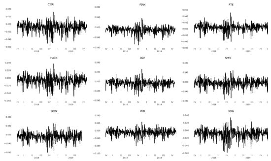
Figure 1.
Daily excess returns, high-tech ETFs (12/01/2017-1/31/2020).
The BDS test of Brock, Dechert, and Scheinkman was run to confirm the nonlinearity of the series as described in [73]. The results (see Table A2 in the Appendix A) suggest that we can reject the hypothesis of linearity in this sense, while nonlinearity is confirmed.
We also determine whether the analyzed series are stationary by using the Augmented Dickey–Fuller (ADF) test, proposed by Dickey and Fuller [74], and the Phillips–Perron (PP) test [75]. A stationary time series is mean-reverting and has a finite variance that guarantees that the process will never drift too far away from the mean. Table A3 in the Appendix A shows the results of the ADF test and the PP test for the daily logarithmic returns. The hypothesis of a unit root is rejected for all the variables at 90%, 95%, and 99% of confidence, which implies that the excess returns of price levels are stationary.
5.2. Constructing the Idiosyncratic Volatility Measure
The idiosyncratic volatility measure was estimated as specified in Section 3.4. The results are available in Table A4 in the Appendix A.
In Figure 2, where the resulting idiosyncratic volatility measures are plotted, we can observe similar trends or an association between all nine high-tech ETFs. High volatility occurred with greater spikes during the fourth quarter of 2018. A mean comparison for the idiosyncratic volatility measure was performed between the range of 2018 and 2019. The average mean for the studied high-tech ETFs reported for this measure in 2018 and 2019 is 0.0017 and 0.0014, respectively, implying a decrease of 13%.
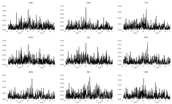
Figure 2.
Daily Idiosyncratic Volatility Measure, high-tech ETFs (12/01/2017-1/31/2020).
Having estimated the one-factor market model structure and confirmed the robustness of the model, we proceed by using the constructed idiosyncratic volatility measure in our MRS model to measure the relationship between the expected excess return and the constructed idiosyncratic volatility of the ETFs.
5.3. Heteroscedastic MRS (1,1) for Idiosyncratic Volatility and Return
In this section we present the results of the Heteroscedastic MRS model to analyze the relationship between idiosyncratic and excess return in the context of emerging technologies.
Multiple breakpoint Bai–Perron tests of 1 to M globally determined breaks was executed. For four of the nine ETFs the test indicated the existence of 1 break. The results can be consulted in Appendix A Table A5. For simplicity, we assume that the nine ETFs present a high and a low volatility regime. The results of the Heteroscedastic MRS model are shown in Table 2.
Table 2.
Heteroscedastic Markov regime-switching (MRS) for high-tech ETFs excess returns, individual idiosyncratic risk, and excess return in two regimes.
The Wald Test is performed for the model coefficient associated to idiosyncratic risk, to test the null hypothesis, which states that the mean idiosyncratic risk in both regimes combined equals zero. The null hypothesis can be rejected for all associated coefficients for the nine models. The results are shown in Table A6 in the Appendix A. The Wald Test was also run to test equality between the idiosyncratic risk, Log(Sigma) and the mean coefficient in the high volatility regime versus the low volatility regime. The null hypothesis can be rejected for all nine models for idiosyncratic volatility and Log(Sigma) coefficient, as reported in Table A7 and Table A8 in the Appendix A. The equality test for the mean can be rejected for only two models as shown in Table A9 in the Appendix A.
For comparative purposes, the same idiosyncratic risk and excess return structure was modelled with a GARCH(1,1) in order to check the goodness of fit. The GARCH(1,1) model output is shown in Table A10 in the Appendix A and the root mean square error (RMSE) measure, log likelihood statistic and Akaike information criterion (AIC) are shown for comparative purposes in Table A11 in the Appendix A. The results indicate that the Heteroscedastic MRS model is preferable than the GARCH model.
A heteroscedastic MRS model was estimated to analyze the relationship between idiosyncratic risk and excess return in the context of emerging technologies.
Idiosyncratic volatility and excess return are not constant in time, for they are regime dependent. MRS involving time series analysis was therefore suitable for this study. The coefficient of interest is related to the independent idiosyncratic risk variable that explains the excess return for each individual high-tech ETF.
For all nine ETFs, a high volatility and a low volatility regime were identified. From the estimated heteroscedastic MRS model we can observe that the coefficients related to the idiosyncratic risk are statistically significant at 99% confidence, indicating that idiosyncratic risk matters for ETF excess returns. The standard deviation for the high volatility regime is 0.0140 and for the low volatility regime is 0.0084.
In the high volatility regime, the estimated coefficients are negative and in the low volatility regime the estimated coefficients are positive for eight of the nine ETFs. For the remaining one, FTE ETF, the associated coefficient is negative in the low volatility regime, but not statistically significant.
These findings indicate that idiosyncratic risk is relevant in explaining returns in the context of high-tech ETFs and that the sign of the relationship is volatility dependent, having a negative relationship in high volatility periods and a positive relationship in low volatility periods.
Higher idiosyncratic risk hence leads to lower excess return during high volatility and to higher excess returns during low volatility and higher excess returns for the studied ETFs during low volatility regimes.
The Markov-chain transition probability shows how ETF prices fluctuate across the regimes. We observed that the probabilities of transiting from one state to another are lower than the probabilities of remaining in the same regime.
The average probabilities of the nine high-tech ETFs staying in the high and low volatility regimes are 64% and 62%, respectively. The probabilities of transit from the high volatility regime to the low volatility regime and vice versa are 36% and 37%, respectively.
The likelihood of each regime remaining in the same regime interval demonstrates the presence of a moderate volatility clustering among the excess returns of ETFs. In other words, a high volatility observation is preceded by a low volatility observation, and vice versa; also, no re-estimation of the two-regime heteroscedastic MRS model with restrictions on the transition matrix was required since none of the transition probabilities have near-zero values.
Regarding the expected duration of regimes, the average for the high volatility regime is four days and for the low volatility regime is five days, which is aligned with the behavior of the high-tech sector subject to short-term noise across stock markets.
Overall, the results indicate that the heteroscedastic MRS models for the nine high-tech ETFs identify and distinguish between several sources of volatility clustering, where regime persistence implies that if the unconditional variance is high in one regime, then the phases of high volatility tend to cluster together due to that regime persistence [76]. This shows that volatility clustering is moderately caused by the persistence of the high volatility regime.
Figure 3, Figure 4, Figure 5, Figure 6, Figure 7, Figure 8, Figure 9, Figure 10 and Figure 11 show the filtered and smooth probability plots for the nine high-tech ETFs. The heteroscedastic MRS (1,1) models cause switching between regimes for all nine high-tech ETFs, which are consistent with the probabilities of staying and switching. Hence, association between regimes can be crucial to capture volatility clustering. Figure 3, Figure 4, Figure 5, Figure 6, Figure 7, Figure 8, Figure 9, Figure 10 and Figure 11 also indicate similar patterns across the nine high-tech ETFs where, as expected, the probability of the ETF price return is slightly higher in a low volatility regime than in a high volatility regime, indicating that ETFs can be used to a certain extent as hedging tools.
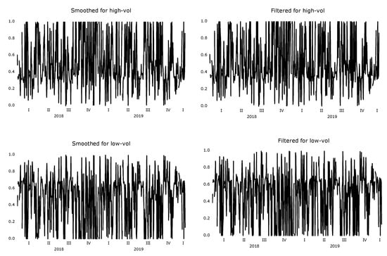
Figure 3.
Computed smoothed probabilities and filtered conditional volatilities for CIBR.
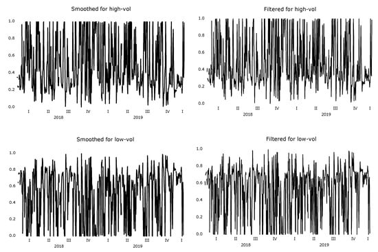
Figure 4.
Computed smoothed probabilities and filtered conditional volatilities for FINX.
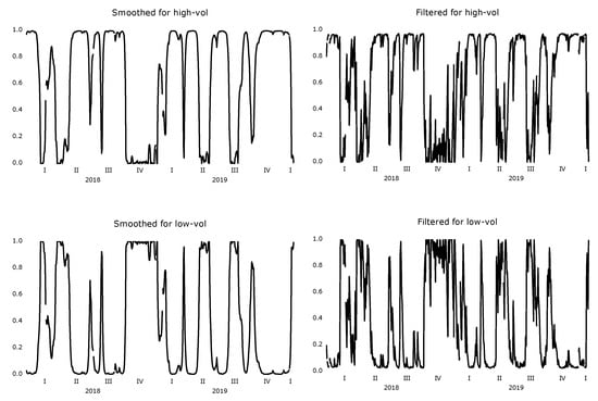
Figure 5.
Computed smoothed probabilities and filtered conditional volatilities for FTE.
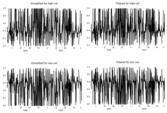
Figure 6.
Computed smoothed probabilities and filtered conditional volatilities for HACK.
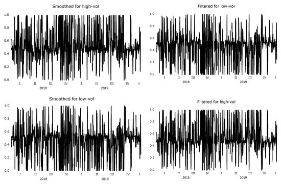
Figure 7.
Computed smoothed probabilities and filtered conditional volatilities for IGV.
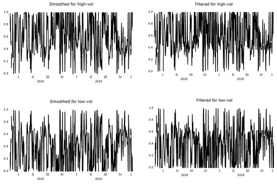
Figure 8.
Computed smoothed probabilities and filtered conditional volatilities for SMH.
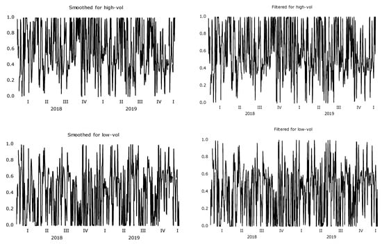
Figure 9.
Computed smoothed probabilities and filtered conditional volatilities for SOXX.
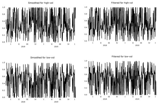
Figure 10.
Computed smoothed probabilities and filtered conditional volatilities for XSD.
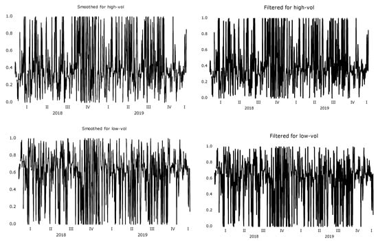
Figure 11.
Computed smoothed probabilities and filtered conditional volatilities for XSW.
These results provide empirical support for the idea that under-diversified investors are not compensated for not holding diversified portfolios in high volatility regimes, as opposed to low volatility regimes, where compensation for not holding a diversified portfolio does occur. The benefits of diversification vary across the studied period, which also implies that the number of stocks required for a specific diversification level also varies.
These facts suggest that investors do not rationally diversify the risk under certain market conditions in the context of the emerging technology sector. One area requiring further examination is the role of information arriving in the market. Excess volatility peaks precisely during periods associated to uncertainty [77], such as radical technological changes, and therefore the resulting fundamental information is less useful for making predictions about future values [77]. Moreover, high-tech firms suffer from the asymmetric information problem [16,78,79], which may also explain why investors do not seem to necessarily diversify their portfolios rationally under certain market conditions.
6. Conclusions
We investigate the relationship between idiosyncratic risk and return among nine high-tech ETFs using daily return data for the 12/01/2017–1/31/2020 period using idiosyncratic volatility as a proxy for idiosyncratic risk. According to the fundamental theory, idiosyncratic risks can be eliminated through diversification and hence should not be priced, though the empirical evidence is mixed.
To further investigate these relationships, time series analysis and a heteroscedastic MRS model were used because the results obtained are not constant over time. Two regimes were identified, namely those of high and low volatility.
By studying the relationship between excess return and idiosyncratic volatility we found that a negative relationship between idiosyncratic risk and return prevails during the high volatility regime, while in low volatility regimes a positive relationship is identified for eight of the nine high-tech ETFs.
The results are partially aligned with the predominant theory that idiosyncratic risk is priced positively and suggest that firm-specific risk matters for ETF pricing and indeed for the underlying index pricing of the high-tech sector. High-tech investment therefore seems to entail a higher or lower idiosyncratic risk and a negative or positive effect on the high-tech ETF returns during different regimes.
This indicates that investors do require a greater risk premium for being more exposed to idiosyncratic risk during low volatility in the high-tech sector. However, during high volatility periods, compensation for such exposure does not occur.
There are relevant implications for investors. In the high-tech sector, the return and idiosyncratic risk can play an important role in risk diversification and allocation, thus leading to changes across volatility regimes. However, idiosyncratic risk might not necessarily reflect a risk premium and lead to inconclusive price inference. The adjustment of returns by idiosyncratic risk should be considered when evaluating performance with benchmarks. If portfolio managers ignore idiosyncratic risk, this may lead to under-diversification of those portfolios, and given the recent evidence that idiosyncratic risk and the number of stocks needed to achieve a specific level of diversification have increased, those implications require even greater attention.
The results also indicate that the idiosyncratic component impacts market returns and drives the predictability of the expected returns of high-tech companies. Adding ETFs from the high-tech sector to a portfolio does not necessarily lead to risk reduction, since the patterns between idiosyncratic volatility and return are similar, and regime dependent.
This article makes the following new contributions to the idiosyncratic volatility literature: First, it documents a significant relationship between idiosyncratic risk and return in the high-tech sector, contrary to the fundamental theory of investment that generally states that idiosyncratic risk should not be priced since it can be eliminated through diversification. Second, it provides evidence that idiosyncratic risk is priced negatively or positively depending on volatility regimes in the IT context. Third, the results highlight how investors do not diversify the risk rationally under certain market circumstances.
This article also provides insights into the role of pricing of managed funds, especially for funds exposed to equity investment, and has important implications for investors and international institutions that include high-tech investment portfolios in their decision-making. This paper is merely the first step towards determining the scope of excess return and idiosyncratic volatility for purposes of asset pricing in the high-tech sector, and its conclusions are therefore tentative.
Future work will cover the analyzed sectors in a broader manner, including a comparative view of ETFs versus underlying assets, and will improve the database by extending the sample over time. Areas for further research include the actual portfolio implications of changes in idiosyncratic risk and return.
Author Contributions
Conceptualization, L.A.; Data curation, L.A.; Formal analysis, L.A.; Investigation, L.A.; Methodology, L.A.; Validation, L.A.; Writing—original draft, L.A. and A.M.G.-L.; Writing—review–editing, L.A. and A.M.G.-L. All authors have read and agreed to the published version of the manuscript.
Funding
This research received no external funding.
Institutional Review Board Statement
Not applicable.
Informed Consent Statement
Not applicable.
Data Availability Statement
The estimated and test results data presented in this study are available on request from the corresponding author. Publicly available datasets were analyzed in this study. This data can be found here: www.finance.yahoo.com (accessed on 15 November 2020).
Acknowledgments
The authors wish to thank The Royal Academy of Economic and Financial Sciences of Spain and to Sigfrido Iglesias for his valuable feedback.
Conflicts of Interest
The authors declare no conflict of interest.
Appendix A
Table A1.
ETF Specifications.
Table A2.
BDS Test for Nonlinearity for ETF excess return.
Table A3.
Unit Root Test for ETF excess return.
Table A4.
Generalized autoregressive conditional heteroskedastic (GARCH) (1,1) one-factor model for constructing the idiosyncratic volatility measure.
Table A5.
Multiple breakpoint Bai–Perron tests for ETF excess return.
Table A6.
WALD Test for idiosyncratic risk coefficient combined.
Table A7.
WALD Test for the idiosyncratic risk coefficient.
Table A8.
WALD Test for the LOG(SIGM) coefficient.
Table A9.
WALD Test for the mean.
Table A10.
GARCH (1,1) model of ETF idiosyncratic risk and excess return.
Table A11.
Comparing GARCH vs. Heteroscedastic MRS, root mean square error (RMSE), Log Likelihood, AIC for Idiosyncratic Risk vs. Return.
References
- Sharpe, W. Capital Asset Prices: A Theory of Market Equilibrium Under Conditions of Risk. J. Financ. 1964, 19, 425–442. [Google Scholar] [CrossRef]
- Lintner, J. Security Prices, Risk, and Maximal Gains from Diversificatio. J. Financ. 1965, 20, 587–615. [Google Scholar] [CrossRef]
- Black, F. Capital Market Equilibrium with Restricted Borrowing. J. Bus. 1972, 45, 444–455. [Google Scholar] [CrossRef]
- Tinic, S.M.; West, R.R. Risk, Return, and Equilibrium: A Revisit. J. Political Econ. 1986, 94, 126–147. [Google Scholar] [CrossRef]
- Goyal, A.; Santa-Clara, P. Idiosyncratic Risk Matters. J. Financ. 2003, 58, 975–1007. [Google Scholar] [CrossRef]
- Fu, F. Idiosyncratic risk and the cross-section of expected stock returns. J. Financ. Econ. 2009, 91, 24–37. [Google Scholar] [CrossRef]
- Merton, R.C. A Simple Model of Capital Market Equilibrium with Incomplete Information. J. Financ. 1987, 42, 483–510. [Google Scholar] [CrossRef]
- Ang, A.; Hodrick, R.J.; Xing, Y.; Zhang, X. The Cross-Section of Volatility and Expected Returns. J. Financ. 2006, 61, 259–299. [Google Scholar] [CrossRef]
- Ang, A.; Hodrick, R.J.; Xing, Y.; Zhang, X. High Idiosyncratic Volatility and Low Returns: International and Further US Evidence. J. Financ. Econ. 2009, 91, 1–23. [Google Scholar] [CrossRef]
- Campbell, J.; Martin, L.; Burton, G.; Malkiel, Y.X. Have Individual Stocks Become More Volatile? An Empirical Exploration of Idiosyncratic Risk. J. Financ. 2001, 56, 1–43. [Google Scholar] [CrossRef]
- Kearney, C.; Potì, V. Have European Stocks Become more Volatile? An Empirical Investigation of Idiosyncratic and Market Risk in the Euro Area. Eur. Financ. Manag. 2008, 14, 419–444. [Google Scholar] [CrossRef]
- Mazzucato, M.; Tancioni, M. Innovation and Idiosyncratic Risk: An Industry-and Firm-Level Analysis. Ind. Corp. Chang. 2008, 17, 779–811. [Google Scholar] [CrossRef]
- Bagella, M.; Becchetti, L.; Adriani, F. Observed and “Fundamental” Price–Earning Ratios: A Comparative Analysis of High-Tech Stock Evaluation in the US and in Europe. J. Int. Money Financ. 2005, 24, 549–581. [Google Scholar] [CrossRef][Green Version]
- Chan, L.K.C.; Lakonishok, J.; Sougiannis, T. The Stock Market Valuation of Research and Development Expenditures. J. Financ. 2001, 56, 2431–2456. [Google Scholar] [CrossRef]
- Schwert, G.W. Stock Volatility in the New Millennium: How Wacky is Nasdaq? J. Monet. Econ. 2002, 49, 3–26. [Google Scholar] [CrossRef]
- Gharbi, S.; Sahut, J.-M.; Teulon, F. R&D Investments and High-Tech Firms’ Stock Return Volatility. Technol. Forecast. Soc. Chang. 2014, 88, 306–312. [Google Scholar] [CrossRef]
- Domanski, D. Idiosyncratic Risk in the 1990s: Is It an IT Story? WIDER Working Paper Series DP; World Institute for Development Economic Research (UNU-WIDER): Helsinki, Finland, 2003. [Google Scholar]
- Ben-David, I.; Franzoni, F.; Moussawi, R. ETFs, Arbitrage, and Contagion; Swiss Finance Inst.: Zurich, Switzerland, 2012. [Google Scholar]
- Ben-David, I.; Franzoni, F.; Moussawi, R. Do ETFs Increase Volatility? J. Financ. 2018, 73, 2471–2535. [Google Scholar] [CrossRef]
- Li, F.W.; Teo, S.W.M.; Yang, C.C. ETF Momentum; Research Collection Lee Kong Chian School of Business: Singapore, 2019; pp. 1–51. Available online: https://ink.library.smu.edu.sg/lkcsb_research/6446 (accessed on 28 March 2021).
- Borah, N.; Pan, L.; Park, J.C.; Nan, S. Does Corporate Diversification Reduce Value in High Technology Firms? Rev. Quant. Financ. Account. 2018, 51, 683–718. [Google Scholar] [CrossRef]
- Fornari, F.; Pericoli, M. Characteristics of Stock Prices in TMT and Traditional Sectors. Banca d’Italia Temi Discuss 2001, (unpublished). [Google Scholar]
- Ahmed, M.S.; Alhadar, M. Momentum, Asymmetric Volatility and Idiosyncratic Risk-Momentum Relation: Does Technology-Sector Matter? Q. Rev. Econ. Financ. 2020, 78, 355–371. [Google Scholar] [CrossRef]
- Brown, J.R.; Martinsson, G.; Petersen, B.C. Stock Markets, Credit Markets, and Technology-Led Growth. J. Financ. Intermediation 2017, 32, 45–59. [Google Scholar] [CrossRef]
- Junttila, J.; Kallunki, J.-P.; Kärja, A.; Martikainen, M. Stock Market Response to Analysts’ Perceptions and Earnings in a Technology-Intensive Environment. Int. Rev. Financ. Anal. 2005, 14, 77–92. [Google Scholar] [CrossRef]
- Kwon, S.S.; Yin, Q.J. Executive Compensation, Investment Opportunities, and Earnings Management: High-Tech Firms Versus Low-Tech Firms. J. Account. Audit. Financ. 2006, 21, 119–148. [Google Scholar] [CrossRef]
- Kwon, S.S.; Yin, J. A Comparison of Earnings Persistence in High-Tech and Non-High-Tech Firms. Rev. Quant. Financ. Account. 2015, 44, 645–668. [Google Scholar] [CrossRef]
- Lim, E.N.K. The Role of Reference Point in CEO Restricted Stock and its Impact on R&D Intensity in High-Technology Firms. Strateg. Manag. J. 2015, 36, 872–889. [Google Scholar] [CrossRef]
- Watanabe, C.; Hur, J.Y.; Lei, S. Converging Trend of Innovation Efforts in High Technology Firms Under Paradigm Shift—a Case of Japan’s Electrical Machinery. Omega 2006, 34, 178–188. [Google Scholar] [CrossRef]
- Kothari, S.P.; Laguerre, T.E.; Leone, A.J. Capitalization versus Expensing: Evidence on the Uncertainty of Future Earnings from Capital Expenditures Versus R&D Outlays. Rev. Account. Stud. 2002, 7, 355–382. [Google Scholar] [CrossRef]
- Hall, B.H. The Financing of Research and Development. Oxf. Rev. Econ. Policy 2002, 18, 35–51. [Google Scholar] [CrossRef]
- Upadhyay, A.; Zeng, H. Cash Holdings and the Bargaining Power of R&D-Intensive Targets. Rev. Quant. Financ. Account. 2017, 49, 885–923. [Google Scholar] [CrossRef]
- Aboody, D.; Lev, B. Information Asymmetry, R&D, and Insider Gains. J. Financ. 2000, 55, 2747–2766. [Google Scholar] [CrossRef]
- Jones, C.M.; Rhodes-Kropf, M. The Price of Diversifiable Risk in Venture Capital and Private Equity; Working Paper; Columbia University: New York, NY, USA, 2003. [Google Scholar]
- Lehmann, B.N. Residual Risk Revisited. J. Econ. 1990, 45, 71–97. [Google Scholar] [CrossRef]
- Jiang, X.; Lee, B.-S. The Dynamic Relation between Returns and Idiosyncratic Volatility. Financ. Manag. 2006, 35, 43–65. [Google Scholar] [CrossRef]
- Malkiel, B.G.; Xu, Y. Idiosyncratic Risk and Security Returns. SSRN 2006. [Google Scholar] [CrossRef]
- Levy, H. Equilibrium in an Imperfect Market: A Constraint on the Number of Securities in the Portfolio. Am. Econ. Rev. 1978, 68, 643–658. [Google Scholar]
- Spiegel, M.I.; Wang, X. Cross-Sectional Variation in Stock Returns: Liquidity and Idiosyncratic Risk. SSRN 2005. Available online: https://ssrn.com/abstract=709781 (accessed on 28 March 2021).
- Chua, C.T.; Choo, Y.J.G.; Zhe, Z. Idiosyncratic Volatility Matters for the Cross-Section of Returns-in More Ways Than One; Singapore Management University: Singapore, 2006. [Google Scholar]
- Switzer, L.N.; Picard, A. Idiosyncratic Volatility, Momentum, Liquidity, and Expected Stock Returns in Developed and Emerging Markets. Multinatl. Financ. J. 2015, 19, 169–221. [Google Scholar] [CrossRef]
- Rachwalski, M.; Wen, Q. Idiosyncratic Risk Innovations and the Idiosyncratic Risk-Return Relation. Rev. Asset Pricing Stud. 2016, 6, 303–328. [Google Scholar] [CrossRef]
- Barberis, N.; Huang, M. Mental Accounting, Loss Aversion, and Individual Stock Returns. J. Financ. 2001, 56, 1247–1292. [Google Scholar] [CrossRef]
- Bali, T.G.; Cakici, N. Idiosyncratic Volatility and the Cross Section of Expected Returns. J. Financ. Quant. Anal. 2008, 43, 29–58. [Google Scholar] [CrossRef]
- Huang, W.; Qianqiu, L.S.; Ghon, R.L.Z. Return Reversals, Idiosyncratic Risk, and Expected Returns. Rev. Financ. Stud. 2010, 23, 147–168. [Google Scholar] [CrossRef]
- Han, Y.; Lesmond, D. Liquidity Biases and the Pricing of Cross-Sectional Idiosyncratic Volatility. Rev. Financ. Stud. 2011, 24, 1590–1629. [Google Scholar] [CrossRef]
- Bali, T.G.; Cakici, N.; Whitelaw, R.F. Maxing Out: Stocks as Lotteries and the Cross-Section of Expected Returns. J. Financ. Econ. 2011, 99, 427–446. [Google Scholar] [CrossRef]
- Boyer, B.; Mitton, T.; Vorkink, K. Expected Idiosyncratic Skewness. Rev. Financ. Stud. 2010, 23, 169–202. [Google Scholar] [CrossRef]
- Nartea, G.V.; Ward, B.D. Does Idiosyncratic Risk Matter? Evidence from the Philippine Stock Market. AJBA 2017, 2, 47–67. [Google Scholar]
- Brockman, P.; Yan, X. The Time-Series Behavior and Pricing of Idiosyncratic Volatility: Evidence from 1926–1962; University of Missouri: Columbia, MI, USA, 2008. [Google Scholar] [CrossRef]
- Barber, B.M.; Odean, T. Trading is Hazardous to Your Wealth: The Common Stock Investment Performance of Individual Investors. J. Financ. 2000, 55, 773–806. [Google Scholar] [CrossRef]
- Benartzi, S.; Thaler, R.H. Naive Diversification Strategies in Defined Contribution Saving Plans. Am. Econ. Rev. 2001, 91, 79–98. [Google Scholar] [CrossRef]
- Falkenstein, E.G. Preferences for Stock Characteristics as Revealed by Mutual Fund Portfolio Holdings. J. Financ. 1996, 51, 111–135. [Google Scholar] [CrossRef]
- Di Iorio, A.; Liu, B. Idiosyncratic Volatility and Momentum: The Performance of Australian Equity Pension Funds; University of Wollongong: Wollongong, NSW, Australia, 2015. [Google Scholar]
- Engel, R.F. Autoregressive Conditional Heteroscedasticity with Estimates of the Variance of United Kingdom Inflation. Econometrica 1982, 50, 987–1007. [Google Scholar] [CrossRef]
- Bollerslev, T. Generalized Autoregressive Conditional Heteroskedasticity. J. Econom. 1986, 31, 307–327. [Google Scholar] [CrossRef]
- Richards, A.J. Idiosyncratic Risk: An Empirical Analysis, with Implications for the Risk of Relative-Value Trading Strategies. SSRN (November, 1999). IMF Working Paper No. 99/148. Available online: https://ssrn.com/abstract=880675 (accessed on 28 March 2021).
- Angelidis, T. Idiosyncratic Risk in Emerging Markets. Financ. Rev. 2010, 45, 1053–1078. [Google Scholar] [CrossRef]
- Hamao, Y.; Mei, J.; Xu, Y. Idiosyncratic Risk and the Creative Destruction in Japan; NBER Working Paper No. 9642; NBER: Cambridge, MA, USA, 2003. [Google Scholar]
- Lamourex, C.G.; Lastrapes, W.D. Heteroskedasticity in Stock Return Data: Volume versus Garch Effects. J. Financ. 1990, 45, 221–229. [Google Scholar] [CrossRef]
- Mizrach, B. Learning and Conditional Heteroscedasticity in Asset Returns; Departmental Working Papers 199526; Rutgers University, Department of Economics: New Brunswick, NJ, USA, 1996. [Google Scholar]
- Stock, J. Estimating Continuous Time Processes Subject to Time Deformation. J. Am. Stat. Assoc. 1988, 83, 77–85. [Google Scholar] [CrossRef][Green Version]
- Ang, A.; Timmermann, A. Regime Changes and Financial Markets. Annu. Rev. Financ. Econ. 2012, 4, 313–337. [Google Scholar] [CrossRef]
- Ang, A.; Bekaert, G. How Regimes Affect Asset Allocation. Financ. Anal. J. 2004, 60, 86–99. [Google Scholar] [CrossRef]
- Guidolin, M.; Timmermann, A. International Asset Allocation Under Regime Switching, Skew, and Kurtosis Preferences. Rev. Financ. Stud. 2008, 21, 889–935. [Google Scholar] [CrossRef]
- Kritzman, M.; Page, S.; Turkington, D. Regime Shifts: Implications for Dynamic Strategies (Corrected). Financ. Anal. J. 2012, 68, 22–39. [Google Scholar] [CrossRef]
- Dou, P.Y.; David, R.; Gallagher, M.; David, S.; Terry, S. Cross-Region and Cross-Sector Asset Allocation with Regimes. Acc. Financ. 2014, 54, 809–846. [Google Scholar] [CrossRef]
- Jiang, P.; Liu, Q.; Tse, Y. International Asset Allocation with Regime Switching: Evidence from the ETFs. Asia-Pac. J. Financ. Stud. 2015, 44, 661–687. [Google Scholar] [CrossRef]
- Quandt, R.E. The Estimation of the Parameters of a Linear Regression System Obeying Two Separate Regimes. J. Am. Stat. Assoc. 1958, 53, 873–880. [Google Scholar] [CrossRef]
- Goldfeld, S.M.; Quandt, R.E. A Markov Model for Switching Regressions. J. Econom. 1973, 1, 3–15. [Google Scholar] [CrossRef]
- Hamilton, J.D. A New Approach to the Economic Analysis of Nonstationary Time Series and the Business Cycle. Econ. J. Econ. Soc. 1989, 57, 357–384. [Google Scholar] [CrossRef]
- Yahoo Finance. Available online: www.finance.yahoo.com (accessed on 15 November 2020).
- Brock, W.A.; Scheinkman, J.A.; Dechert, W.D.; LeBaron, B. A Test for Independence Based on the Correlation Integral; Technical Report; University of Wisconsin-Madison: Madison, WI, USA, 1986. [Google Scholar]
- Dickey, D.A.; Fuller, W.A. Likelihood Ratio Statistics for Autoregressive Time Series with a Unit Root. Econ. J. Econ. Soc. 1981, 49, 1057–1072. [Google Scholar] [CrossRef]
- Phillips, P.C.B.; Perron, P. Testing for a Unit Root in Time Series Regression. Biometrika 1988, 75, 335–346. [Google Scholar] [CrossRef]
- Gray, S.F. Modeling the conditional distribution of interest rates as a regime-switching process. J. Financ. Econ. 1996, 42, 27–62. [Google Scholar] [CrossRef]
- Barron, D.; Byard, O.E.; Kile, C.; Riedl, E.J. Hightechnology Intangibles and Analysts’ Forecasts. J. Account. Res. 2002, 40, 289–312. [Google Scholar] [CrossRef]
- Gu, F.; Li, J.Q. The Credibility of Voluntary Disclosure and Insider Stock Transactions. J. Account. Res. 2007, 45, 771–810. [Google Scholar] [CrossRef]
- Gu, F.; Wang, W. Intangible Assets, Information Complexity, and Analysts’ Earnings Forecasts. J. Bus. Financ. Account. 2005, 32, 1673–1702. [Google Scholar] [CrossRef]


Publisher’s Note: MDPI stays neutral with regard to jurisdictional claims in published maps and institutional affiliations. |
© 2021 by the authors. Licensee MDPI, Basel, Switzerland. This article is an open access article distributed under the terms and conditions of the Creative Commons Attribution (CC BY) license (https://creativecommons.org/licenses/by/4.0/).