Tails of the Moments for Sums with Dominatedly Varying Random Summands

Abstract

The asymptotic behaviour of the tail expectation $\mathbb{E}\left({\left(S_n^{\xi }\right)}^{\alpha }{\mathrm{𝕝}}_{\{S_n^{\xi }>x\}}\right)$ is investigated, where exponent $\alpha$ is a nonnegative real number and $S_n^{\xi }={\xi }_1+\dots +{\xi }_n$ is a sum of dominatedly varying and not necessarily identically distributed random summands, following a specific dependence structure. It turns out that the tail expectation of such a sum can be asymptotically bounded from above and below by the sums of expectations $\mathbb{E}\left({\xi }_i^{\alpha }{\mathrm{𝕝}}_{\{{\xi }_i>x\}}\right)$ with correcting constants. The obtained results are extended to the case of randomly weighted sums, where collections of random weights and primary random variables are independent. For illustration of the results obtained, some particular examples are given, where dependence between random variables is modelled in copulas framework.

1. Introduction

Let $n\in \mathbb{N}:=\{1,2,\dots \}$ and let us consider two collections of random variables (r.v.s): heavy-tailed (see definition in Section 2) r.v.s $\{{\xi }_1,\dots ,{\xi }_n\}$, called primary r.v.s, and nonnegative, non-degenerate at zero r.v.s $\{{\theta }_1,\dots ,{\theta }_n\}$, called random weights. In this paper, we investigate the asymptotic behaviour of the sums of primary r.v.s

$$S_n^{\xi }:=\sum _{k=1}^n{\xi }_k={\xi }_1+\dots +{\xi }_n,$$

(1)

and their weighted counterparts, namely randomly weighted sums

$$S_n^{\theta \xi }:=\sum _{k=1}^n{\theta }_k{\xi }_k={\theta }_1{\xi }_1+\dots +{\theta }_n{\xi }_n.$$

(2)

Asymptotics of (1) and (2) have been studied extensively during recent years in the literature of applied probability under various different assumptions about collections $\{{\xi }_1,\dots ,{\xi }_n\}$, $\{{\theta }_1,\dots ,{\theta }_n\}$ and their dependence structures. In particular, there are many papers addressing the asymptotic behaviour of the tail probabilities

$$\mathbb{P}\left(S_n^{\xi }>x\right)\mathrm{and}\mathbb{P}\left(S_n^{\theta \xi }>x\right)$$

(3)

expressing them by the sums of tail probabilities of individual summands, i.e., ${\sum }_{k=1}^n\mathbb{P}\left({\xi }_k>x\right)$ and ${\sum }_{k=1}^n\mathbb{P}\left({\theta }_k{\xi }_k>x\right)$, respectively (see, e.g., [1,2,3,4,5,6,7,8,9,10,11]). The main results from the majority of the aforementioned papers are reviewed in detail in Section 3. In line with the tail probabilities $\mathbb{P}\left(S_n^{\xi }>x\right)$ and $\mathbb{P}\left(S_n^{\theta \xi }>x\right)$, asymptotics of the tail expectations $\mathbb{E}\left(S_n^{\xi }{\mathrm{𝕝}}_{\{S_n^{\xi }>x\}}\right)$ and $\mathbb{E}\left(S_n^{\theta \xi }{\mathrm{𝕝}}_{\{S_n^{\theta \xi }>x\}}\right)$ are investigated in the literature; however, the number of papers is relatively scarce (see [6,7,12] and the references therein).

In this paper, inspired by the recent results by Leipus et al. [7], we are particularly interested in the asymptotics of the tail expectations

$$\mathbb{E}\left({\left(S_n^{\xi }\right)}^{\alpha }{\mathrm{𝕝}}_{\{S_n^{\xi }>x\}}\right)\mathrm{and}\mathbb{E}\left({\left(S_n^{\theta \xi }\right)}^{\alpha }{\mathrm{𝕝}}_{\{S_n^{\theta \xi }>x\}}\right),$$

(4)

where $\alpha$ is a nonnegative real number. We assume that r.v.s ${\xi }_1,\dots ,{\xi }_n$ are not necessarily identically distributed, belong to the class of dominatedly varying distributions (see Section 2.2), a subclass of heavy-tailed distributions, and follow a specific dependence structure, called pairwise quasi-asymptotic independence (see Section 2.3). We seek to asymptotically bound the tail expectations (4) by the sums of individual tail expectations $\mathbb{E}\left({{\xi }_k}^{\alpha }{\mathrm{𝕝}}_{\{{\xi }_k>x\}}\right)$ and $\mathbb{E}\left({\left({\theta }_k{\xi }_k\right)}^{\alpha }{\mathrm{𝕝}}_{\{{\theta }_k{\xi }_k>x\}}\right)$, respectively, with some specific correcting constants (see Theorems 3 and 4).

Although our paper is more of a theoretical kind, it is worth noting that sums of the form (1) and, especially, (2) are often encountered in the practical applications of probability in financial and actuarial context. One example stems from the so-called discrete time risk model, in which primary r.v. ${\xi }_k$ could correspond to the net losses (total claim amount minus total premium income) of an insurance company during period $(k-1,k]$, calculated at the moment k, and random weight ${\theta }_k$ could correspond to the stochastic discount factor, from the moment k to the present moment 0, for all $k=1,\dots ,n$. In such a scenario, sum $S_n^{\theta \xi }$ could be treated as the present value of a total discounted net loss of a company in the time interval $(0,n]$ (for more details, see, e.g., [5,8,10,13,14,15,16]).

Other insurance related application is based on the individual risk model [17]. Say that an insurance company has a portfolio consisting of n policies. Then, we could interpret $S_n^{\theta \xi }$ as the total claim amount incurred from the whole insurance portfolio. Here, ${\theta }_k{\xi }_k$, $k\in \{1,\dots ,n\}$ would correspond to the claim amount from the kth policy. Since there is a possibility that no claim will be incurred, ${\theta }_k$ is an indicatory Bernoulli r.v. which represents the occurrence of the kth claim (${\theta }_k=1$ if the claim has occurred and zero otherwise) and r.v. ${\xi }_k$ corresponds to the claim size of the kth policy given that the payment was made (see [18] and Chapter 4 of [19] as well).

Tang and Yuan [15] considered an example related to the construction of investment portfolio and capital allocation. Suppose that there are n distinct asset classes or lines of business, from which the portfolio is formed. Then, r.v. ${\xi }_k$ could correspond to the loss incurred from the kth instrument. As for the role of random weights, there could be different viewpoints: ${\theta }_k$ could be treated as a stochastic discount factor of the kth asset class or, for instance, as a weight corresponding to the kth instrument in the portfolio. Then, random sum $S_n^{\theta \xi }$ would correspond to the present value of total loss of a portfolio at the present moment in the former case, and total weighted portfolio loss in the latter.

Highly related to the portfolio construction discussed above are various risk measures quantifying the underlying risk of the portfolio—we list several of them below, which are commonly encountered in the literature of risk management (see, e.g., [20,21]) and in which the asymptotic results concerning tail probabilities and tail expectations could be useful:

• Value-at-Risk (VaR) at level $q\in (0,1)$:

  $${\mathrm{VaR}}_q\left(S_n^{\xi }\right)=inf\left\{x\in \mathbb{R}\mid \mathbb{P}\left(S_n^{\xi }>x\right)⩽1-q\right\}.$$
• Conditional tail expectation (CTE) at level $q\in (0,1)$:

  $${\mathrm{CTE}}_q\left(S_n^{\xi }\right)=\mathbb{E}\left(S_n^{\xi }\mid S_n^{\xi }>{\mathrm{VaR}}_q\left(S_n^{\xi }\right)\right).$$

For the above risk measures, the asymptotic behaviour is mainly considered as $q\uparrow 1$. Nevertheless, as mentioned in [22]: “as the excessive prudence of the current regulatory framework requires a confidence level close to 1, the notion of Extreme Value Theory becomes appropriate”. In other words, q being close to 1 results in large ${\mathrm{VaR}}_q\left(S_n^{\xi }\right)$ values. For more about the estimation of the aforementioned risk measures, see the works of Yang et al. [12], Tang and Yuan [15], Asimit et al. [22], Hua and Joe [23] and Wang et al. [24] (and the references therein).

The rest of the paper is structured as follows. In Section 2, we review the basic definitions of the heavy-tailed distributions and introduce the reader to the specific dependence structure used in this paper. In Section 3, we discuss the related results in literature. In Section 4, our main results, which allow to asymptotically bound the tail expectations (4), are presented and later proved in Section 5. Finally, as applications of our result, in Section 6, we provide three different examples of random sums, for which dependence is controlled via a copula, in a bivariate setting.

2. Definitions and Preliminaries

2.1. Notational Conventions

Before delving into more details, we briefly introduce the notations used throughout the paper. All limiting relationships and asymptotic estimates, unless stated otherwise, are understood as x approaches infinity. For two positive functions f and g, we write:

• $f\left(x\right)\lesssim g\left(x\right)$ if $lim\; sup\frac{f\left(x\right)}{g\left(x\right)}⩽1$
• $f\left(x\right)=o\left(g\right(x\left)\right)$ if $lim\frac{f\left(x\right)}{g\left(x\right)}=0$
• $f\left(x\right)=O\left(g\right(x\left)\right)$ if $lim\; sup\frac{f\left(x\right)}{g\left(x\right)}<\infty$
• $f\left(x\right)\sim g\left(x\right)$ if $lim\frac{f\left(x\right)}{g\left(x\right)}=1$
• $f\left(x\right)\asymp g\left(x\right)$ if $0<lim\; inf\frac{f\left(x\right)}{g\left(x\right)}⩽lim\; sup\frac{f\left(x\right)}{g\left(x\right)}<\infty$

For any r.v. X, by $F_X\left(x\right)$, we denote the distribution function (d.f.) of X, i.e., $F_X\left(x\right)=\mathbb{P}(X⩽x)$. By $\overline{F}\left(x\right)$, we denote the tail function of d.f. F, i.e., $\overline{F}\left(x\right)=1-F\left(x\right)$. By $F^{*n}\left(x\right)$, we write the n-fold convolution of a d.f. F. That is, if $X_1,\dots ,X_n$ are independent copies of X, then $F_X^{*n}\left(x\right)=\mathbb{P}(X_1+\dots +X_n⩽x)$, and $\overline{F_X^{*n}}\left(x\right)=\mathbb{P}(X_1+\dots +X_n>x)$.

We say that r.v. X has an infinite right support if ${\overline{F}}_X\left(x\right)>0$ for all $x\in \mathbb{R}$. In addition, we say that d.f. F is supported on $\mathbb{R}$ if $\overline{F}\left(x\right)>0$ for all $x\in \mathbb{R}$. We write ${\mathrm{𝕝}}_A$ to denote the indicator function of an event A. For any r.v. X, by $X^{+}$ and $X^{-}$, we denote its positive and negative parts, respectively: $X^{+}=max\{X,0\}$, $X^{-}=max\{-X,0\}$. For a given $x\in \mathbb{R}$, by $\lfloor x\rfloor$, we denote the integer part of x and, by $\widehat{x}=x-\lfloor x\rfloor$, we denote the fractional part of x.

2.2. Heavy-Tailed Distributions

In this subsection, we recall the main classes of heavy-tailed distributions. At first, we present the class of dominatedly varying distributions $\mathcal{D}$, which is a central one in this paper.

• A d.f. F supported on $\mathbb{R}$ is said to be dominatedly varying (belong to class $\mathcal{D}$) if $\underset{x\to \infty }{lim\; sup}\frac{\overline{F}\left(xy\right)}{\overline{F}\left(x\right)}<\infty$ for any (for some) $y\in (0,1)$.

As noted in [25], Peter and Paul distribution is an example of a distribution belonging to the class $\mathcal{D}$. We say that r.v. X is distributed according to the generalised Peter and Paul distribution with parameters $(a,b)$, where $b>1$, $a\in (0,\infty )$, if its tail is characterised by the following equality

$${\overline{F}}_X\left(x\right)=(b^a-1)\sum _{k⩾1,b^k>x}{b}^{-ak}.$$

Since ${\overline{F}}_X\left(x\right)={\left(b^{-a}\right)}^{⌊{log}_{b}x⌋}$ for $x⩾1$, we get that

$$\begin{array}{c}\hfill \underset{x\to \infty }{lim\; sup}\frac{{\overline{F}}_X\left(xy\right)}{{\overline{F}}_X\left(x\right)}=\underset{x\to \infty }{lim\; sup}{\left(b^{-a}\right)}^{⌊{log}_{b}x+{log}_{b}y⌋-⌊{log}_{b}x⌋}⩽{\left(b^{-a}\right)}^{⌊{log}_{b}y⌋-1}.\end{array}$$

for any $y\in (0,1)$, implying $F_X\in \mathcal{D}$.

Class $\mathcal{D}$ is not the only subclass of heavy-tailed distributions. Below, we briefly recall the other classes of heavy-tailed distributions and describe the relationships between them.

• A d.f. F is said to be heavy-tailed (belong to class $\mathcal{H}$) if for any $\alpha >0$

  $${\int }_{-\infty }^{\infty }{\mathrm{e}}^{\alpha x}\mathrm{d}F\left(x\right)=\infty .$$
• A d.f. F is said to be long tailed (belong to class $\mathcal{L}$) if for any $y>0$ $\overline{F}(x+y)\sim \overline{F}\left(x\right)$.
• A d.f. F supported on $\mathbb{R}$ is said to be subexponential (belong to class $\mathcal{S}$) if $F\in \mathcal{L}$ and $\overline{F^{*2}}\left(x\right)\sim 2\overline{F}\left(x\right).$
• A d.f. F is said to be regularly varying with coefficient $\alpha ⩾0$ (belong to class ${\mathcal{R}}_{\alpha }$) if for any $y>0$

  $$\underset{x\to \infty }{lim}\frac{\overline{F}\left(xy\right)}{\overline{F}\left(x\right)}=y^{-\alpha }.$$
• A d.f. F is said to be consistently varying (belong to class $\mathcal{C}$) if

  $$\underset{y\uparrow 1}{lim}\underset{x\to \infty }{lim\; sup}\frac{\overline{F}\left(xy\right)}{\overline{F}\left(x\right)}=1.$$

The class of consistently varying distributions $\mathcal{C}$ is the largest subclass of a class $\mathcal{D}$. The following example of a distribution belonging to $\mathcal{C}\backslash {\bigcup }_{\alpha ⩾0}{\mathcal{R}}_{\alpha }$ is given in [26]. Let Y and N be independent r.v.s such that $Y\stackrel{d}{=}\mathcal{U}\left([0,1]\right)$ and N is geometric r.v. with parameter $p\in (0,1)$, i.e., $\mathbb{P}(N=k)=(1-p)p^k$ for $k=0,1,\dots$). Then, r.v. $\xi$ defined by

$$\begin{array}{c}\hfill \xi =(1+Y)2^N\end{array}$$

(5)

belongs to the class $\mathcal{C}$ but not to the class ${\bigcup }_{\alpha ⩾0}{\mathcal{R}}_{\alpha }$. This fact can be derived from the expression

$$\begin{array}{c}\hfill F_{\xi }\left(x\right)=\left(1-p\right)\left(\frac{1-p^{\lfloor {log}_{2}x\rfloor }}{1-p}+\left(\frac{x}{2^{\lfloor {log}_{2}x\rfloor }}-1\right)p^{\lfloor {log}_{2}x\rfloor }\right){\mathrm{𝕝}}_{\{x⩾1\}}.\end{array}$$

(6)

In summary, the interrelationships of the heavy-tailed distribution classes can be expressed by the following relations

$$\mathcal{R}:=\bigcup _{\alpha ⩾0}{\mathcal{R}}_{\alpha }⊊\mathcal{C}⊊\mathcal{L}\cap \mathcal{D}\cap \mathcal{S}⊊\mathcal{L}⊊\mathcal{H};\mathcal{D}⊊\mathcal{H};\mathcal{D}\not\subset \mathcal{S}.$$

Some of the above relationships follow directly from the definitions, while proofs of the others can be found in, e.g., [25,27,28,29,30], ([31] Sections 6.1 and 6.2) and [32].

The classes $\mathcal{C}$ and $\mathcal{D}$ can be characterised by specific indices. We recall these important indices. The first one is a so-called L-index, used in, e.g., [6,7,11,33,34]. The $L_F$ index for d.f. F is

$$L_F:=\underset{y\downarrow 1}{lim}\underset{x\to \infty }{lim\; inf}\frac{\overline{F}\left(xy\right)}{\overline{F}\left(x\right)}.$$

The second important index is the upper Matuszewska index introduced in [35]. In this paper, we stick with the slightly different but equivalent formulation given in [36] and used in many other articles (e.g., [2,6,8,11,34]). For a d.f. F, the upper Matuszewska index$J_F^{+}$ is

$$J_F^{+}:=\underset{y>1}{inf}\left\{-\frac{1}{logy}log\left\{\underset{x\to \infty }{lim\; inf}\frac{\overline{F}\left(xy\right)}{\overline{F}\left(x\right)}\right\}\right\}.$$

The aforementioned indices give important characterisations for dominatedly varying and consistently varying d.f.s (see, e.g., [33], Proposition 1.1):

$$L_F>0\iff F\in \mathcal{D}\iff J_F^{+}<\infty ;L_F=1\iff F\in \mathcal{C}.$$

For a r.v. $\xi$ with d.f. $F_{\xi }$, we write for brevity: $L_{\xi }=L_{F_{\xi }}$ and $J_{\xi }^{+}=J_{F_{\xi }}^{+}$. More information on classes $\mathcal{C}$ and $\mathcal{D}$ can be found in Chapter 2 of [36] and the discussion in Section 3 of [27].

2.3. QAI Dependence Structure

We now introduce the main dependence assumption about r.v.s ${\xi }_1,\dots ,{\xi }_n$ used in this paper, so-called pairwise quasi-asymptotic independence, which is due to Chen and Yuen [2].

• R.v.s $\{{\xi }_1,\dots ,{\xi }_n\}$ with infinite right supports are called pairwise quasi-asymptotically independent (pQAI) if for any $k,l\in \{1,\dots ,n\}$, $k\ne l$,

  $$\underset{x\to \infty }{lim}\frac{\mathbb{P}\left({\xi }_k^{+}>x,{\xi }_l^{+}>x\right)}{\mathbb{P}\left({\xi }_k^{+}>x\right)+\mathbb{P}\left({\xi }_l^{+}>x\right)}=\underset{x\to \infty }{lim}\frac{\mathbb{P}\left({\xi }_k^{+}>x,{\xi }_l^{-}>x\right)}{\mathbb{P}\left({\xi }_k^{+}>x\right)+\mathbb{P}\left({\xi }_l^{+}>x\right)}=0.$$

  (7)

Let us construct two examples of r.v.s possessing such a dependence structure using copulas.

Example 1.

Let $\{{\xi }_1,\dots ,{\xi }_n\}$ be r.v.s with infinite right supports and corresponding marginal d.f.s $\{F_1,\dots ,F_n\}$. Consider the Farlie–Gumbel–Morgenstein (FGM) copula:

$$C_{\vartheta }(u,v)=uv+\vartheta uv(1-u)(1-v),u,v\in [0,1],\vartheta \in \left[-1,1\right].$$

Let r.v.s ${\xi }_i$, ${\xi }_j$ have a joint d.f. $\mathbb{P}\left({\xi }_i⩽x_1,{\xi }_j⩽x_2\right)=C_{{\vartheta }_i}(F_i\left(x_1\right),F_j\left(x_2\right))$ with some ${\vartheta }_i\in [-1,1]$ if $max\{i,j\}-min\{i,j\}=1$, $min\{i,j\}=2k-1$ for some $k\in \mathbb{N}$ and be independent otherwise. Then, r.v.s $\{{\xi }_1,\dots ,{\xi }_n\}$ are pQAI.

It follows from Sklar’s theorem (see [37,38] Theorem 2.3.3)) that for any given marginal d.f.s $F_1$, $F_2$ and an arbitrary copula $C(u_1,u_2)$, function $F(x_1,x_2):=C(F_1\left(x_1\right)$, $F_2\left(x_2\right))$ is a bivariate d.f. with marginal d.f.s $F_1$, $F_2$. If ${\xi }_i$, ${\xi }_j$, $i,j=1,\dots n$ are independent, then obviously they are pQAI. If $max\{i,j\}-min\{i,j\}=1$, $min\{i,j\}=2k-1$ for some $k\in \mathbb{N}$, then

$$\begin{array}{cc}\hfill \frac{\mathbb{P}\left({\xi }_i>x,{\xi }_j>x\right)}{\mathbb{P}\left({\xi }_i>x\right)+\mathbb{P}\left({\xi }_j>x\right)}& =\frac{1-F_i\left(x\right)-F_j\left(x\right)+C_{{\vartheta }_i}\left(F_i\left(x\right),F_j\left(x\right)\right)}{{\overline{F}}_i\left(x\right)+{\overline{F}}_j\left(x\right)}\hfill \\ \hfill & =\frac{{\overline{F}}_i\left(x\right){\overline{F}}_j\left(x\right)\left(1+{\vartheta }_i{F}_i\left(x\right)F_j\left(x\right)\right)}{{\overline{F}}_i\left(x\right)+{\overline{F}}_j\left(x\right)}⩽2{\overline{F}}_i\left(x\right).\hfill \end{array}$$

(8)

Similarly, by observing that

$$\begin{array}{c}\hfill \mathbb{P}\left({\xi }_i>x,{\xi }_j^{-}>x\right)⩽\mathbb{P}\left({\xi }_i>x,{\xi }_j^{-}⩾x\right)=\mathbb{P}\left({\xi }_j⩽-x\right)-\mathbb{P}\left({\xi }_i⩽x,{\xi }_j⩽-x\right)\end{array}$$

for positive x, we get

$$\begin{array}{cc}\hfill \frac{\mathbb{P}({\xi }_i>x,{\xi }_j^{-}>x)}{\mathbb{P}\left({\xi }_i>x\right)+\mathbb{P}\left({\xi }_j>x\right)}& ⩽\frac{F_j(-x)-C_{{\vartheta }_i}\left(F_i\left(x\right),F_j(-x)\right)}{{\overline{F}}_i\left(x\right)+{\overline{F}}_j\left(x\right)}\hfill \\ & =\frac{{\overline{F}}_i\left(x\right)F_j(-x)\left(1-{\vartheta }_i{F}_i\left(x\right)F_j(-x)\right)}{{\overline{F}}_i\left(x\right)+{\overline{F}}_j\left(x\right)}⩽2F_j(-x).\hfill \end{array}$$

(9)

Estimates (8) and (9) imply (7). Consequently, r.v.s $\{{\xi }_1,\dots ,{\xi }_n\}$ in Example 1 are pQAI.

In a more general setting, one can consider n-dimensional ($n⩾2$) Farley–Gumbel–Morgenstein (FGM) distributions (for a detailed treatment on this type of distributions see, e.g., [39]). For r.v.s $\{{\xi }_1,\dots ,{\xi }_n\}$ with corresponding marginal d.f.s $\{F_1,\dots ,F_n\}$, n-variate FGM d.f. is defined as follows:

$$\mathbb{P}\left({\xi }_1⩽x_1,\dots ,{\xi }_n⩽x_n\right)=\prod _{i=1}^n{F}_i\left(x_i\right)\left(1+\sum _{1⩽i<j⩽n}{\vartheta }_{ij}{\overline{F}}_i\left(x_i\right){\overline{F}}_j\left(x_j\right)\right),$$

(10)

where parameters ${\vartheta }_{ij}$, $i,j\in \{1,\dots ,n\}$ should satisfy the following condition

$$1+\sum _{1⩽i<j⩽n}{\epsilon }_i{\epsilon }_j{\vartheta }_{ij}⩾0,$$

(11)

for all ${\epsilon }_i=-{sup}_{x\in \mathbb{R}}\left\{F_i\left(x\right)\right\}\backslash \{0,1\}$ or ${\epsilon }_i=1-{inf}_{x\in \mathbb{R}}\left\{F_i\left(x\right)\right\}\backslash \left\{0,1\right\}$ (see [39] Chapter 44, Section 13). Necessary condition (11) is required for (10) to be a well defined d.f..

Note that, if we assume that random vector $({\xi }_1,\dots ,{\xi }_n)$ is distributed according to (10) in our example, r.v.s ${\xi }_1,\dots ,{\xi }_n$ are still pQAI, since bivariate marginal distributions of random vectors $({\xi }_i,{\xi }_j)$, $i,j\in \{1,\dots ,n\}$, $i<j$ are distributed according to a bivariate FGM distribution with marginal d.f.s $F_i$, $F_j$ and FGM copula. Indeed, from (10), we get

$$\begin{array}{cc}\hfill \mathbb{P}\left({\xi }_i⩽x_1,{\xi }_j⩽x_2\right)& =\mathbb{P}\left({\xi }_1⩽\infty ,\dots ,{\xi }_i⩽x_1,\dots ,{\xi }_j⩽x_2,\dots ,{\xi }_n⩽\infty \right)\hfill \\ \hfill & =F_i\left(x_1\right)F_j\left(x_2\right)\left(1+{\vartheta }_{ij}{\overline{F}}_i\left(x_1\right){\overline{F}}_j\left(x_2\right)\right).\hfill \end{array}$$

Example 2.

Let ${\xi }_1$, ${\xi }_2$ be r.v.s with corresponding d.f.s $F_1$, $F_2$ and let random vector $({\xi }_1,{\xi }_2)$ have a bivariate d.f. $F(x_1,x_2):=C_{\vartheta }(F_1\left(x_1\right),F_2\left(x_2\right))$, where $C_{\vartheta }$ is the Ali–Michail–Haq copula [40]:

$$C_{\vartheta }(u,v)=\frac{uv}{1-\vartheta (1-u)(1-v)},u,v\in [0,1],\vartheta \in (-1,1).$$

Similarly to in Example 1, it can be shown that r.v.s ${\xi }_1$, ${\xi }_2$ are QAI.

Indeed, for positive x, we have

$$\begin{array}{cc}\hfill \frac{\mathbb{P}\left({\xi }_1>x,{\xi }_2>x\right)}{\mathbb{P}\left({\xi }_1>x\right)+\mathbb{P}\left({\xi }_2>x\right)}& =\frac{1-F_1\left(x\right)-F_2\left(x\right)+C_{\vartheta }\left(F_1\left(x\right),F_2\left(x\right)\right)}{{\overline{F}}_1\left(x\right)+{\overline{F}}_2\left(x\right)}\hfill \\ \hfill & =\frac{{\overline{F}}_1\left(x\right){\overline{F}}_2\left(x\right)\left(1+\vartheta \left(F_2\left(x\right)-{\overline{F}}_1\left(x\right)\right)\right)}{({\overline{F}}_1\left(x\right)+{\overline{F}}_2\left(x\right))(1-\vartheta {\overline{F}}_1\left(x\right){\overline{F}}_2\left(x\right))}⩽\frac{2{\overline{F}}_2\left(x\right)}{1-\vartheta {\overline{F}}_1\left(x\right){\overline{F}}_2\left(x\right)}.\hfill \end{array}$$

In the same fashion for positive x, we obtain

$$\begin{array}{cc}\hfill \frac{\mathbb{P}({\xi }_1>x,{\xi }_2^{-}>x)}{\mathbb{P}\left({\xi }_1>x\right)+\mathbb{P}\left({\xi }_2>x\right)}& ⩽\frac{F_2(-x)-C_{\vartheta }\left(F_1\left(x\right),F_2(-x)\right)}{{\overline{F}}_1\left(x\right)+{\overline{F}}_2\left(x\right)}\hfill \\ \hfill & =\frac{F_2(-x){\overline{F}}_1\left(x\right)\left(1-\vartheta {\overline{F}}_2(-x)\right)}{({\overline{F}}_1\left(x\right)+{\overline{F}}_2\left(x\right))(1-\vartheta {\overline{F}}_1\left(x\right){\overline{F}}_2(-x))}⩽\frac{2F_2(-x)}{1-\vartheta {\overline{F}}_1\left(x\right){\overline{F}}_2(-x)}.\hfill \end{array}$$

The derived estimates imply that r.v.s ${\xi }_1$ and ${\xi }_2$ are QAI.

For more about copulas applications in problems related to modelling dependence of heavy-tailed distributions, the reader may refer to the works of Albrechter et al. [41], Asimit et al. [22], Fang et al. [42], Yang et al. [43] and Wang et al. [24] (and the references therein). For a systematic treatment of copulas theory see, for instance, the work of Nelsen [38]. In the next section, we recall briefly more similar dependence structures between r.v.s and examine their relations to pQAI condition (7).

3. Related Results

In this section, we briefly review some of the related results found in the literature, regarding the asymptotic behaviour of the tail probability and tail expectation of random sums in the form of either (1) or (2). Throughout the section, unless mentioned otherwise, we assume that the collections of r.v.s $\{{\xi }_1,\dots ,{\xi }_n\}$ and $\{{\theta }_1,\dots ,{\theta }_n\}$ are independent.

3.1. Asymptotics of Tail Probabilities

There are many papers in which r.v.s ${\xi }_1,\dots ,{\xi }_n$ are assumed to be independent or identically distributed, see, for instance, the works of Tang and Tsitshiashivili [8], Goovaertz et al. [5], Wang et al. [9] and Wang and Tang [10] (and the references therein). In this subsection, however, we concentrate on the results in which such restrictive assumptions have been weakened.

We start with several results in which the exact asymptotic equivalence

$$\mathbb{P}\left(S_n^{\xi }>x\right)\sim \sum _{k=1}^n{\overline{F}}_{{\xi }_k}\left(x\right)$$

(12)

was obtained.

Geluk and Tang [4] achieved (12) for distributions $F_{{\xi }_k}\in \mathcal{D}\cap \mathcal{S}$ (see [4] Theorem 3.1). It was assumed that r.v.s ${\xi }_1,\dots ,{\xi }_n$ satisfy the so-called Assumption A (as in [4]), which was referred to later as a strong quasi-asymptotic independence in other articles (e.g., [6,7,16,44]), as well.

• R.v.s ${\xi }_1,\dots ,{\xi }_n$ with infinite right supports are called pairwise strongly quasi-asymptotically independent (pSQAI) if for any $k,l\in \{1,\dots n\}$, $k\ne l$,

  $$\underset{min\{x_k,x_l\}\to \infty }{lim}\mathbb{P}\left(|{\xi }_k|>x_k\mid {\xi }_l>x_l\right)=0.$$

Nearly at the same time, Chen and Yuen [2] achieved (12) (see [2] Theorem 3.1) in the smaller class $\mathcal{C}$, but this time the pSQAI condition was replaced by the similar pQAI condition (see Section 2.3). We observe that pSQAI condition implies pQAI. Indeed, by arbitrarily choosing ${\xi }_k$, ${\xi }_l$, $1⩽k\ne l⩽n$, we get that

$$\begin{array}{c}\hfill \mathbb{P}\left(|{\xi }_k|>x_k\mid {\xi }_l>x_l\right)=\mathbb{P}({\xi }_k^{+}>x_k\mid {\xi }_l>x_l)+\mathbb{P}({\xi }_k^{-}>x_k\mid {\xi }_l>x_l)\to 0,\end{array}$$

as $min\{x_k,x_l\}\to \infty$. Thus, it follows that

$$\begin{array}{cc}\hfill \underset{x\to \infty }{lim}\frac{\mathbb{P}({\xi }_k^{+}>x,{\xi }_l^{+}>x)}{\mathbb{P}({\xi }_k^{+}>x)+\mathbb{P}({\xi }_l^{+}>x)}& ⩽\underset{x\to \infty }{lim}\mathbb{P}\left({\xi }_k>x\mid {\xi }_l>x\right)=0,\hfill \end{array}$$

and, in the same way,

$$\begin{array}{cc}\hfill \underset{x\to \infty }{lim}\frac{\mathbb{P}({\xi }_k^{-}>x,{\xi }_l^{+}>x)}{\mathbb{P}({\xi }_k^{+}>x)+\mathbb{P}({\xi }_l^{+}>x)}& ⩽\underset{x\to \infty }{lim}\mathbb{P}\left({\xi }_k^{-}>x\mid {\xi }_l>x\right)=0.\hfill \end{array}$$

Moreover, in the same article by Chen and Yuen, the results are extended to the case of randomly weighted sums (see [2] Theorem 3.2), resulting in relation

$$\mathbb{P}\left(S_n^{\theta \xi }>x\right)\sim \sum _{k=1}^n{\overline{F}}_{{\theta }_k{\xi }_k}\left(x\right)$$

under the following moment condition on random weights:

$$max\{\mathbb{E}{\theta }_1^p\dots ,\mathbb{E}{\theta }_n^p\}<\infty \mathrm{for}\mathrm{some}p>max\{J_{{\xi }_1}^{+},\dots ,J_{{\xi }_n}^{+}\}.$$

(13)

Later, inspired by the results of Chen and Yuen, Yi et al. [11] considered the tail probability asymptotics of the randomly weighted sum $S_n^{\theta \xi }$, when r.v.s ${\xi }_1,\dots ,{\xi }_n$ belong to the class $\mathcal{D}$ and follow the same pQAI structure (see [11] Theorems 1 and 2). It was shown that under (13) and additional tail assumption

$$\underset{x\to \infty }{lim}\frac{{\overline{F}}_{{\xi }_k^{-}}\left(x\right)}{{\overline{F}}_{{\xi }_k}\left(x\right)}=0\mathrm{for}\mathrm{all}k\in \{1,\dots ,n\},$$

(14)

the following asymptotic bounds hold:

$$L_n^{\xi }\sum _{k=1}^n{\overline{F}}_{{\theta }_k{\xi }_k}\left(x\right)\lesssim \mathbb{P}\left(S_n^{\theta \xi }>x\right)\lesssim \frac{1}{L_n^{\xi }}\sum _{k=1}^n{\overline{F}}_{{\theta }_k{\xi }_k}\left(x\right),$$

(15)

where $L_n^{\xi }:=min\left\{L_{{\xi }_1},\dots ,L_{{\xi }_n}\right\}$. Cheng [3] managed to tighten the bounds in (15) (see [3] Theorems 1.1 and 1.2) by putting the L-indices inside the sums and obtaining

$$\sum _{k=1}^n{L}_{{\xi }_k}{\overline{F}}_{{\theta }_k{\xi }_k}\left(x\right)\lesssim \mathbb{P}\left(S_n^{\theta \xi }>x\right)\lesssim \sum _{k=1}^n\frac{1}{L_{{\xi }_k}}{\overline{F}}_{{\theta }_k{\xi }_k}\left(x\right),$$

where $F_{{\xi }_k}\in \mathcal{D}$ for all $k\in \{1,\dots ,n\}$. The assumption (13) was substituted by a weaker condition (see [3] Assumption C and Remark 1.1):

$$\underset{x\to \infty }{lim}\frac{F_{{\theta }_k{\xi }_k}\left(x\right)}{F_{{\xi }_k}\left(x\right)}=0\mathrm{for}\mathrm{all}k\in \{1,\dots ,n\}.$$

Moreover, instead of pQAI, two other dependence structures, namely pairwise tail quasi-asymptotic independence (see [3] Assumption B) and pairwise asymptotic independence, together with condition (14) (see [3] Assumption A) were considered.

• R.v.s ${\xi }_1,\dots ,{\xi }_n$ with infinite right supports are called pairwise tail quasi-asyptotically independent (pTQAI) if for any $k,l=1,\dots ,n$, $k\ne l$,

  $$\begin{array}{cc}\hfill \underset{min\{x_k,x_l\}\to \infty }{lim}\frac{\mathbb{P}({\xi }_k^{+}>x_k,{\xi }_l^{+}>x_l)}{\mathbb{P}({\xi }_k^{+}>x_k)+\mathbb{P}({\xi }_l^{+}>x_l)}& =\underset{min\{x_k,x_l\}\to \infty }{lim}\frac{\mathbb{P}({\xi }_k^{-}>x_k,{\xi }_l^{+}>x_l)}{\mathbb{P}({\xi }_k^{+}>x_k)+\mathbb{P}({\xi }_l^{+}>x_l)}=0.\hfill \end{array}$$
• R.v.s ${\xi }_1,\dots ,{\xi }_n$ with infinite right supports are called pairwise asymptotically independent (pAI) if for any $k,l=1,\dots ,n$, $k\ne l$,

  $$\begin{array}{c}\hfill \underset{x\to \infty }{lim}\frac{\mathbb{P}({\xi }_k>x,{\xi }_l>x)}{\mathbb{P}({\xi }_k>x)}=\underset{x\to \infty }{lim}\frac{\mathbb{P}({\xi }_k>x,{\xi }_l>x)}{\mathbb{P}({\xi }_l>x)}=0.\end{array}$$

As noted in [3], implication $\mathrm{pTQAI}\Rightarrow \mathrm{pQAI}$ follows trivially, by allowing $x_k$ and $x_l$ to attain the same value x in the definition of pTQAI. It is easy to see that pAI implies pQAI if r.v.s ${\xi }_1,\dots ,{\xi }_n$ are nonnegative. Nonetheless, (14) is a sufficient condition for $\mathrm{pAI}\Rightarrow \mathrm{pQAI}$ to hold in the general case because, for any $1⩽k\ne l⩽n$,

$$\begin{array}{c}\hfill \underset{x\to \infty }{lim}\frac{\mathbb{P}({\xi }_k>x,{{\xi }_l}^{-}>x)}{\mathbb{P}({\xi }_k>x)+\mathbb{P}({\xi }_l>x)}⩽\underset{x\to \infty }{lim}\frac{F_{{\xi }_l}(-x)}{{\overline{F}}_{{\xi }_l}\left(x\right)}=0.\end{array}$$

Quite recently, Jaunė et al. [6] reconsidered the asymptotic behaviour of tail probability $\mathbb{P}\left(S_n^{\theta \xi }>x\right)$ under the pQAI condition on r.v.s ${\xi }_1,\dots ,{\xi }_n$ in the class $\mathcal{D}$. The statement of Lemma 1 from [6] extends mainly the results of Yi et al. [11], resulting in (15) under the moment condition (13), but without the additional assumption (14).

3.2. Asymptotics of Tail Expectations

Having reviewed the main results about the asymptotic behaviour of tail probabilities (3), we now turn to the asymptotics of tail expectation of random sums $S_n^{\xi }$ and $S_n^{\theta \xi }$ which is the main object of this paper. Tang and Yuan [15] obtained the relation

$$\mathbb{E}\left({\theta }_1{\xi }_1{\mathrm{𝕝}}_{\{S_n^{\theta \xi }>x\}}\right)\sim \mathbb{E}\left({\theta }_1{\xi }_1{\mathrm{𝕝}}_{\{{\theta }_1{\xi }_1>x\}}\right)$$

for i.i.d. r.v.s ${\xi }_1,\dots ,{\xi }_n$ from the class $\mathcal{D}\cap \mathcal{S}$ and random weights ${\theta }_1,\dots ,{\theta }_n$, satisfying $\mathbb{E}{\theta }_k^{p_k}<\infty$, $p_k>J_{{\xi }_k}^{+}$, ${\overline{F}}_{{\theta }_k{\xi }_k}\left(x\right)=O\left({\overline{F}}_{{\theta }_1{\xi }_1}\left(x\right)\right)$ for all $k\in \{1,\dots ,n\}$ (see [15] Theorem 4). It was noted by Yang et al. [12] that, under additional condition ${\overline{F}}_{{\theta }_k{\xi }_k}\left(x\right)\asymp {\overline{F}}_{{\theta }_1{\xi }_1}\left(x\right)$ for all $k\in \{1,\dots ,n\}$, relation

$$\mathbb{E}\left(S_n^{\theta \xi }{\mathrm{𝕝}}_{\{S_n^{\theta \xi }>x\}}\right)\sim \sum _{k=1}^n\mathbb{E}\left({\theta }_k{\xi }_k{\mathrm{𝕝}}_{\{{\theta }_k{\xi }_k>x\}}\right)$$

(16)

holds.

Jaunė et al. [6] later weakened the i.i.d. condition of the previous result, allowing pQAI or pSQAI dependence structures among primary r.v.s ${\xi }_1,\dots ,{\xi }_n$, at the cost of exact asymptotics in (16).

Now, we turn to the recent result by Leipus et al. [7], which inspired our investigation. Before stating the relevant theorems, we note that, in [7], the new dependence structure called Assumption $\mathcal{B}$, regarding r.v.s ${\xi }_1,\dots ,{\xi }_n$, is used.

Assumption $\mathcal{B}$. R.v.s ${\xi }_1,\dots ,{\xi }_n$ have infinite right supports and, for all $k,l=1,\dots ,n$, $k\ne l$ satisfy

$$\begin{array}{cc}\hfill \underset{x\to \infty }{lim}\underset{u⩾x}{sup}\mathbb{P}\left({\xi }_k^{+}>x\mid {\xi }_l^{+}>u\right)& =\underset{x\to \infty }{lim}\underset{u⩾x}{sup}\mathbb{P}\left({\xi }_k^{-}>x\mid {\xi }_l^{+}>u\right)\hfill \\ & =\underset{x\to \infty }{lim}\underset{u⩾x}{sup}\mathbb{P}\left({\xi }_k^{+}>x\mid {\xi }_l^{-}>u\right)=0.\hfill \end{array}$$

Similarly, as in the case $\mathrm{pSQAI}\Rightarrow \mathrm{pQAI}$, we can show that Assumption $\mathcal{B}$ implies the pQAI condition because for any ${\xi }_k$, ${\xi }_l$, $1⩽k\ne l⩽n$,

$$\begin{array}{cc}\hfill \underset{x\to \infty }{lim}\frac{\mathbb{P}({\xi }_k^{+}>x,{\xi }_l^{+}>x)}{\mathbb{P}({\xi }_k^{+}>x)+\mathbb{P}({\xi }_l^{+}>x)}& ⩽\underset{x\to \infty }{lim}\underset{u⩾x}{sup}\mathbb{P}\left({\xi }_k^{+}>x\mid {\xi }_l^{+}>u\right)=0,\hfill \\ \hfill \underset{x\to \infty }{lim}\frac{\mathbb{P}({\xi }_k^{-}>x,{\xi }_l^{+}>x)}{\mathbb{P}({\xi }_k^{+}>x)+\mathbb{P}({\xi }_l^{+}>x)}& ⩽\underset{x\to \infty }{lim}\underset{u⩾x}{sup}\mathbb{P}\left({\xi }_k^{-}>x\mid {\xi }_l^{+}>u\right)=0.\hfill \end{array}$$

The following assertion is the main result in [7].

Theorem 1

(See [7] Theorem 4). Let ${\xi }_1,\dots ,{\xi }_n$ be r.v.s satisfying Assumption $\mathcal{B}$ such that $F_{{\xi }_1}\in \mathcal{D}$, $\mathbb{E}{\left|{\xi }_1\right|}^m<\infty$ for some $m\in \mathbb{N}$ and ${\overline{F}}_{{\xi }_k}\left(x\right)\asymp {\overline{F}}_{{\xi }_1}\left(x\right)$, ${\overline{F}}_{{\xi }_k^{-}}\left(x\right)=O\left({\overline{F}}_{{\xi }_1}\left(x\right)\right)$, for all $k=2,\dots ,n$. Then,

$$L_n^{\xi }\sum _{k=1}^n\mathbb{E}\left({\xi }_k^m{\mathrm{𝕝}}_{\{{\xi }_k>x\}}\right)\lesssim \mathbb{E}\left({\left(S_n^{\xi }\right)}^m{\mathrm{𝕝}}_{\{S_n^{\xi }>x\}}\right)\lesssim \frac{1}{L_n^{\xi }}\sum _{k=1}^n\mathbb{E}\left({\xi }_k^m{\mathrm{𝕝}}_{\{{\xi }_k>x\}}\right).$$

Moreover, the results were extended to the general case of weighted sums. This time, however, a quite restrictive assumption about random weights was made; namely, it was supposed that random weights ${\theta }_1,\dots ,{\theta }_n$ are bounded.

Theorem 2

(See [7] Theorem 5). Let ${\xi }_1,\dots ,{\xi }_n$ be r.v.s satisfying Assumption $\mathcal{B}$ such that $F_{{\xi }_1}\in \mathcal{D}$, $\mathbb{E}{\left|{\xi }_1\right|}^m<\infty$ for some $m\in \mathbb{N}$. Let ${\theta }_1,\dots ,{\theta }_n$ be nonnegative, non-degenerate at zero, bounded r.v.s, independent of ${\theta }_1,\dots ,{\theta }_n$. If ${\overline{F}}_{{\theta }_k{\xi }_k}\left(x\right)\asymp {\overline{F}}_{{\theta }_1{\xi }_1}\left(x\right)$, ${\overline{F}}_{{\theta }_k{\xi }_k^{-}}\left(x\right)=O\left({\overline{F}}_{{\theta }_1{\xi }_1}\left(x\right)\right)$, for all $k=2,\dots ,n$. Then,

$$L_n^{\xi }\sum _{k=1}^n\mathbb{E}\left({\left({\theta }_k{\xi }_k\right)}^m{\mathrm{𝕝}}_{\{{\theta }_k{\xi }_k>x\}}\right)\lesssim \mathbb{E}\left({\left(S_n^{\theta \xi }\right)}^m{\mathrm{𝕝}}_{\{S_n^{\theta \xi }>x\}}\right)\lesssim \frac{1}{L_n^{\xi }}\sum _{k=1}^n\mathbb{E}\left({\left({\theta }_k{\xi }_k\right)}^m{\mathrm{𝕝}}_{\{{\theta }_k{\xi }_k>x\}}\right).$$

4. Main Results

In this section we present the main results of this paper. Theorem 3 states the asymptotic bounds for the tail expectation of a random sum $S_n^{\xi }$ and Theorem 4 is mainly a generalisation to the case of randomly weighted sums $S_n^{\theta \xi }$.

We note that Theorems 3 and 4 improve previous results in several ways. For instance, compared to Theorems 1 and 2, we put individual L-indices inside the sums in (17) and (18), thus obtaining more accurate asymptotic bounds. Moreover, we weaken the condition for exponent, from being a nonnegative integer to any nonnegative real number. In addition, Assumption $\mathcal{B}$ considered in [7] is substituted by a weaker pQAI structure and random weights ${\theta }_1,\dots ,{\theta }_n$ need not to be bounded as in Theorem 2. In addition, it is worth noting that, by setting $\alpha =0$ in Theorems 3 and 4, we obtain asymptotics for the tail probabilities (3) (see Remark 2 as well), thus our results can be compared with those discussed in Section 3.1.

Theorem 3.

Let ${\xi }_1,\dots ,{\xi }_n$ be pQAI real-valued r.v.s. If $\mathbb{E}|{\xi }_k{|}^{\alpha }<\infty$, $F_{{\xi }_k}\in \mathcal{D}$ for all $k\in \{1,\dots ,n\}$ and some $\alpha \in [0,\infty )$, then

$$\sum _{k=1}^n{L}_{{\xi }_k}\mathbb{E}\left({\xi }_k^{\alpha }{\mathrm{𝕝}}_{\{{\xi }_k>x\}}\right)\lesssim \mathbb{E}\left({\left(S_n^{\xi }\right)}^{\alpha }{\mathrm{𝕝}}_{\{S_n^{\xi }>x\}}\right)\lesssim \sum _{k=1}^n\frac{1}{L_{{\xi }_k}}\mathbb{E}\left({\xi }_k^{\alpha }{\mathrm{𝕝}}_{\{{\xi }_k>x\}}\right).$$

(17)

Theorem 4.

Let ${\xi }_1,\dots ,{\xi }_n$ be pQAI real valued r.v.s, such that $F_{{\xi }_k}\in \mathcal{D}$ for all $k\in \{1,\dots ,n\}$, and let ${\theta }_1,\dots ,{\theta }_n$ be arbitrarily dependent, nonnegative, non-degenerate at zero r.v.s with

$$max\{\mathbb{E}{\theta }_1^p,\dots ,\mathbb{E}{\theta }_n^p\}<\infty \mathrm{for}\mathrm{some}p>max\{J_{{\xi }_1}^{+},\dots ,J_{{\xi }_n}^{+}\}.$$

If collections $\{{\xi }_1,\dots ,{\xi }_n\}$ and $\{{\theta }_1,\cdots ,{\theta }_n\}$ are independent and $\mathbb{E}{\left({\theta }_k\left|{\xi }_k\right|\right)}^{\alpha }<\infty$ for all $k\in \{1,\dots ,n\}$ and some $\alpha \in [0,\infty )$, then

$$\sum _{k=1}^n{L}_{{\xi }_k}\mathbb{E}\left({\left({\theta }_k{\xi }_k\right)}^{\alpha }{\mathrm{𝕝}}_{\{{\theta }_k{\xi }_k>x\}}\right)\lesssim \mathbb{E}\left({\left(S_n^{\theta \xi }\right)}^{\alpha }{\mathrm{𝕝}}_{\{S_n^{\theta \xi }>x\}}\right)\lesssim \sum _{k=1}^n\frac{1}{L_{{\xi }_k}}\mathbb{E}\left({\left({\theta }_k{\xi }_k\right)}^{\alpha }{\mathrm{𝕝}}_{\{{\theta }_k{\xi }_k>x\}}\right).$$

(18)

Remark 1.

By narrowing the class $\mathcal{D}$ to the class $\mathcal{C}$ of consistently varying distributions (for which the L-index is unit), we get the exact asymptotic equivalence in (18). That is, if $F_{{\xi }_k}\in \mathcal{C}$ for all $k\in \{1,\dots ,n\}$ and all other conditions of Theorem 4 hold, then

$$\sum _{k=1}^n\mathbb{E}\left({\left({\theta }_k{\xi }_k\right)}^{\alpha }{\mathrm{𝕝}}_{\{{\theta }_k{\xi }_k>x\}}\right)\sim \mathbb{E}\left({\left(S_n^{\theta \xi }\right)}^{\alpha }{\mathrm{𝕝}}_{\{S_n^{\theta \xi }>x\}}\right).$$

Remark 2.

When $\alpha =0$, from (18), we obtain asymptotic bounds for tail probabilities:

$$\sum _{k=1}^n{L}_{{\xi }_k}{\overline{F}}_{{\theta }_k{\xi }_k}\left(x\right)\lesssim \mathbb{P}\left(S_n^{\theta \xi }>x\right)\lesssim \sum _{k=1}^n\frac{1}{L_{{\xi }_k}}{\overline{F}}_{{\theta }_k{\xi }_k}\left(x\right).$$

(19)

Remark 3.

Under the same conditions as in Theorem 4, we can obtain asymptotic bounds for the conditional expectation $\mathbb{E}\left({\left(S_n^{\theta \xi }\right)}^{\alpha }\mid S_n^{\theta \xi }>x\right)$. Namely, combining (18) with (19) we obtain the following asymptotic bounds:

$$\begin{array}{cc}\hfill \frac{{\sum }_{k=1}^n{L}_{{\xi }_k}\mathbb{E}\left({\left({\theta }_k{\xi }_k\right)}^{\alpha }{\mathrm{𝕝}}_{\{{\theta }_k{\xi }_k>x\}}\right)}{{\sum }_{k=1}^n\frac{1}{L_{{\xi }_k}}{\overline{F}}_{{\theta }_k{\xi }_k}\left(x\right)}& \lesssim \mathbb{E}\left({\left(S_n^{\theta \xi }\right)}^{\alpha }\mid S_n^{\theta \xi }>x\right)\hfill \\ & \lesssim \frac{{\sum }_{k=1}^n\frac{1}{L_{{\xi }_k}}\mathbb{E}\left({\left({\theta }_k{\xi }_k\right)}^{\alpha }{\mathrm{𝕝}}_{\{{\theta }_k{\xi }_k>x\}}\right)}{{\sum }_{k=1}^n{L}_{{\xi }_k}{\overline{F}}_{{\theta }_k{\xi }_k}\left(x\right)}.\hfill \end{array}$$

(20)

In addition, by using the min–max inequality (22), we can express (20) fully in conditional expectations at the cost of tightness of the initial bounds:

$$\begin{array}{cc}\hfill \underset{1⩽k⩽n}{min}\left\{L_{{\xi }_k}^2\mathbb{E}\left({\left({\theta }_k{\xi }_k\right)}^{\alpha }\mid {\theta }_k{\xi }_k>x\right)\right\}& \lesssim \mathbb{E}\left({\left(S_n^{\theta \xi }\right)}^{\alpha }\mid S_n^{\theta \xi }>x\right)\hfill \\ & \lesssim \underset{1⩽k⩽n}{max}\left\{\frac{1}{L_{{\xi }_k}^2}\mathbb{E}\left({\left({\theta }_k{\xi }_k\right)}^{\alpha }\mid {\theta }_k{\xi }_k>x\right)\right\}.\hfill \end{array}$$

5. Proofs of Main Results

To prove Theorem 3, we need some auxiliary assertions. The lemma below is proved in [7].

Lemma 1.

Let ξ be a real-valued r.v. If $\mathbb{E}{\left({\xi }^{+}\right)}^{\alpha }<\infty$ for some $\alpha \in [0,\infty )$, then for all $x⩾0$.

$$\mathbb{E}\left({\xi }^{\alpha }{\mathrm{𝕝}}_{\{\xi >x\}}\right)=x^{\alpha }\mathbb{P}(\xi >x)+\alpha {\int }_x^{\infty }{u}^{\alpha -1}\mathbb{P}(\xi >u)\mathrm{d}u.$$

The next lemma is crucial for the proof of Theorem 3.

Lemma 2.

Let ${\xi }_1,\dots ,{\xi }_n$ be pQAI real-valued r.v.s, such that $F_{{\xi }_k}\in \mathcal{D}$ for all $k\in \{1,\dots ,n\}$. Then,

$$\sum _{k=1}^n{L}_{{\xi }_k}{\overline{F}}_{{\xi }_k}\left(x\right)\lesssim \mathbb{P}(S_n^{\xi }>x)\lesssim \sum _{k=1}^n\frac{1}{L_{{\xi }_k}}{\overline{F}}_{{\xi }_k}\left(x\right).$$

(21)

Proof. 

The case $n=1$ in (21) follows trivially from the definition of coefficient $L_{{\xi }_1}$. Let $n⩾2$. First, let us consider the upper asymptotic bound in (21).

For an arbitrary $\delta \in (0,1)$,

$$\begin{array}{cc}\hfill \mathbb{P}(S_n^{\xi }>x)& ⩽\sum _{k=1}^n{\overline{F}}_{{\xi }_k}\left((1-\delta )x\right)+\mathbb{P}\left(S_n^{\xi }>x,\bigcap _{k=1}^n\left\{{\xi }_k⩽(1-\delta )x\right\}\right)\hfill \\ \hfill & =:\sum _{k=1}^n{\overline{F}}_{{\xi }_k}\left((1-\delta )x\right)+\mathcal{A}(x,\delta ).\hfill \end{array}$$

By observing that for all $k\in \{1,\cdots ,n\}$

$$\left\{S_n^{\xi }>x,{\xi }_k⩽(1-\delta )x\right\}\subseteq \left\{S_n^{\xi }-{\xi }_k>\delta x\right\},$$

we can estimate the term $\mathcal{A}(x,\delta )$ as follows:

$$\begin{array}{cc}\hfill \mathcal{A}(x,\delta )& ⩽\sum _{k=1}^n\mathbb{P}\left({\xi }_k>\frac{x}{n},S_n^{\xi }-{\xi }_k>\delta x\right)⩽\sum _{k=1}^n\mathbb{P}\left({\xi }_k>\frac{x}{n},\bigcup _{l=1,l\ne k}^n\left\{{\xi }_l>\frac{\delta x}{n-1}\right\}\right)\hfill \end{array}$$

$$\begin{array}{cc}\hfill & ⩽\sum _{k=1}^n\sum _{l=1,l\ne k}^n\mathbb{P}\left({\xi }_k>{\delta }_{1}x,{\xi }_l>{\delta }_{1}x\right),\hfill \end{array}$$

where in the last inequality ${\delta }_1={\delta }_1\left(\delta \right)=min\left\{1/n,\delta /(n-1)\right\}$.

Consequently,

$$\begin{array}{cc}\hfill \frac{\mathbb{P}\left(S_n^{\xi }>x\right)}{{\sum }_{k=1}^n\frac{1}{L_{{\xi }_k}}{\overline{F}}_{{\xi }_k}\left(x\right)}& ⩽\frac{{\sum }_{k=1}^n{\overline{F}}_{{\xi }_k}\left((1-\delta )x\right)}{{\sum }_{k=1}^n\frac{1}{L_{{\xi }_k}}{\overline{F}}_{{\xi }_k}\left(x\right)}+\frac{{\sum }_{k=1}^n{\sum }_{l=1,l\ne k}^n\mathbb{P}\left({\xi }_k>{\delta }_{1}x,{\xi }_l>{\delta }_{1}x\right)}{{\sum }_{k=1}^n\frac{1}{L_{{\xi }_k}}{\overline{F}}_{{\xi }_k}\left(x\right)}\hfill \\ \hfill & =:{\mathcal{I}}_1(x,\delta )+{\mathcal{I}}_2(x,\delta ).\hfill \end{array}$$

Using the min–max inequality,

$$min\left\{\frac{a_1}{b_1},\dots ,\frac{a_m}{b_m}\right\}⩽\frac{a_1+\dots +a_m}{b_1+\dots +b_m}⩽max\left\{\frac{a_1}{b_1},\dots ,\frac{a_m}{b_m}\right\},$$

(22)

provided that $m\in \mathbb{N}$ and $a_i⩾0$, $b_i>0$ for $i=1,\dots ,m$, we get

$$\begin{array}{c}\hfill {\mathcal{I}}_1(x,\delta )⩽\underset{1⩽k⩽n}{max}\left\{L_{{\xi }_k}\frac{{\overline{F}}_{{\xi }_k}\left((1-\delta )x\right)}{{\overline{F}}_{{\xi }_k}\left(x\right)}\right\}.\end{array}$$

Taking into account (22) and observing that

$$\begin{array}{cc}\hfill \sum _{k=1}^n\sum _{l=1,l\ne k}^n\left({\overline{F}}_{{\xi }_k}\left({\delta }_{1}x\right)+{\overline{F}}_{{\xi }_l}\left({\delta }_{1}x\right)\right)& ⩽2(n-1)\sum _{k=1}^n{\overline{F}}_{{\xi }_k}\left({\delta }_{1}x\right),\hfill \end{array}$$

we similarly obtain

$$\begin{array}{cc}\hfill {\mathcal{I}}_2(x,\delta )& =\frac{{\sum }_{k=1}^n{\sum }_{l=1,l\ne k}^n\mathbb{P}\left({\xi }_k>{\delta }_{1}x,{\xi }_l>{\delta }_{1}x\right)}{{\sum }_{k=1}^n{\sum }_{l=1,l\ne k}^n\left({\overline{F}}_{{\xi }_k}\left({\delta }_{1}x\right)+{\overline{F}}_{{\xi }_l}\left({\delta }_{1}x\right)\right)}\hfill \\ & \times \frac{{\sum }_{k=1}^n{\sum }_{l=1,l\ne k}^n\left({\overline{F}}_{{\xi }_k}\left({\delta }_{1}x\right)+{\overline{F}}_{{\xi }_l}\left({\delta }_{1}x\right)\right)}{{\sum }_{k=1}^n\frac{1}{L_{{\xi }_k}}{\overline{F}}_{{\xi }_k}\left(x\right)}\hfill \\ & ⩽\underset{1⩽k\ne l⩽n}{max}\left\{\frac{\mathbb{P}\left({\xi }_k>{\delta }_{1}x,{\xi }_l>{\delta }_{1}x\right)}{{\overline{F}}_{{\xi }_k}\left({\delta }_{1}x\right)+{\overline{F}}_{{\xi }_l}\left({\delta }_{1}x\right)}\right\}\times 2\left(n-1\right)\underset{1⩽k⩽n}{max}\left\{L_{{\xi }_k}\frac{{\overline{F}}_{{\xi }_k}\left({\delta }_{1}x\right)}{{\overline{F}}_{{\xi }_k}\left(x\right)}\right\}.\hfill \end{array}$$

(23)

The fact that $F_{{\xi }_k}\in \mathcal{D}$ for all $k\in \{1,\dots ,n\}$ and condition of pQAI for r.v.s $\left\{{\xi }_1,\dots ,{\xi }_n\right\}$ implies:

$$\begin{array}{cc}\hfill \underset{x\to \infty }{lim\; sup}{\mathcal{I}}_1(x,\delta )& ⩽\underset{1⩽k⩽n}{max}\left\{L_{{\xi }_k}\underset{x\to \infty }{lim\; sup}\frac{{\overline{F}}_{{\xi }_k}\left((1-\delta )x\right)}{{\overline{F}}_{{\xi }_k}\left(x\right)}\right\},\hfill \end{array}$$

(24)

$$\begin{array}{cc}\hfill \underset{x\to \infty }{lim\; sup}{\mathcal{I}}_2(x,\delta )& ⩽2\left(n-1\right)\underset{1⩽k\ne l⩽n}{max}\left\{\underset{x\to \infty }{lim\; sup}\frac{\mathbb{P}\left({\xi }_k>{\delta }_{1}x,{\xi }_l>{\delta }_{1}x\right)}{{\overline{F}}_{{\xi }_k}\left({\delta }_{1}x\right)+{\overline{F}}_{{\xi }_l}\left({\delta }_{1}x\right)}\right\}\hfill \\ & \times \underset{1⩽k⩽n}{max}\left\{L_{{\xi }_k}\underset{x\to \infty }{lim\; sup}\frac{{\overline{F}}_{{\xi }_k}\left({\delta }_{1}x\right)}{{\overline{F}}_{{\xi }_k}\left(x\right)}\right\}=0.\hfill \end{array}$$

(25)

Therefore, by letting $\delta \downarrow 0$, from estimates (24), (25) and definition of indices $L_{{\xi }_k}$, we get the upper bound in (21):

$$\begin{array}{cc}\hfill \underset{x\to \infty }{lim\; sup}\frac{\mathbb{P}(S_n^{\xi }>x)}{{\sum }_{k=1}^n\frac{1}{L_{{\xi }_k}}{\overline{F}}_{{\xi }_k}\left(x\right)}& ⩽1.\hfill \end{array}$$

Let us consider the lower asymptotic bound in (21). Again, choose arbitrary $\delta \in (0,1)$. By the Bonferroni inequality, for this $\delta$, we get

$$\begin{array}{cc}\hfill & \mathbb{P}\left(S_n^{\xi }>x\right)⩾\mathbb{P}\left(S_n^{\xi }>x,\bigcup _{k=1}^n\left\{{\xi }_k>(1+\delta )x\right\}\right)\hfill \\ \hfill & ⩾\sum _{k=1}^n\mathbb{P}\left(S_n^{\xi }>x,{\xi }_k>(1+\delta )x\right)-\sum _{k=1}^n\sum _{l=1,l\ne k}^n\mathbb{P}\left({\xi }_k>(1+\delta )x,{\xi }_l>(1+\delta )x\right)\hfill \\ \hfill & =:{\mathcal{A}}_1(x,\delta )-{\mathcal{A}}_2(x,\delta ).\hfill \end{array}$$

(26)

For the first summand in (26), we obtain

$$\begin{array}{cc}\hfill {\mathcal{A}}_1(x,\delta )& ⩾\sum _{k=1}^n\mathbb{P}\left(S_n^{\xi }-{\xi }_k>-\delta x,{\xi }_k>(1+\delta )x\right)\hfill \\ \hfill & =\sum _{k=1}^n{\overline{F}}_{{\xi }_k}\left((1+\delta )x\right)-\sum _{k=1}^n\mathbb{P}\left(S_n^{\xi }-{\xi }_k⩽-\delta x,{\xi }_k>(1+\delta )x\right)\hfill \\ \hfill & =:{\mathcal{A}}_{11}(x,\delta )-{\mathcal{A}}_{12}(x,\delta ).\hfill \end{array}$$

(27)

For the second term in (27), we get

$$\begin{array}{cc}\hfill {\mathcal{A}}_{12}(x,\delta )& ⩽\sum _{k=1}^n\mathbb{P}\left(\bigcup _{l=1,l\ne k}^n\left\{{\xi }_l⩽-\frac{\delta x}{n-1}\right\},{\xi }_k>(1+\delta )x\right)\hfill \\ \hfill & ⩽\sum _{k=1}^n\sum _{l=1,l\ne k}^n\mathbb{P}\left({\xi }_k>(1+\delta )x,{\xi }_l^{-}⩾\frac{\delta x}{n-1}\right)\hfill \\ \hfill & ⩽\sum _{k=1}^n\sum _{l=1,l\ne k}^n\mathbb{P}\left({\xi }_k>{\delta }_{2}x,{\xi }_l^{-}>{\delta }_{2}x\right),\hfill \end{array}$$

(28)

where ${\delta }_2={\delta }_2\left(\delta \right)=\delta /2(n-1)$ in the last inequality.

We have from (26), (27) and (28) that

$$\begin{array}{cc}\hfill \frac{\mathbb{P}(S_n^{\xi }>x)}{{\sum }_{k=1}^n{L}_{{\xi }_k}{\overline{F}}_{{\xi }_k}\left(x\right)}& ⩾\frac{{\mathcal{A}}_{11}(x,\delta )}{{\sum }_{k=1}^n{L}_{{\xi }_k}{\overline{F}}_{{\xi }_k}\left(x\right)}\hfill \\ & -\frac{{\sum }_{k=1}^n{\sum }_{l=1,l\ne k}^n\mathbb{P}\left({\xi }_k>{\delta }_{2}x,{\xi }_l^{-}⩾{\delta }_{2}x\right)}{{\sum }_{k=1}^n{L}_{{\xi }_k}{\overline{F}}_{{\xi }_k}\left(x\right)}\hfill \\ & -\frac{{\mathcal{A}}_2(x,\delta )}{{\sum }_{k=1}^n{L}_{{\xi }_k}{\overline{F}}_{{\xi }_k}\left(x\right)}\hfill \\ & =:{\mathcal{J}}_1(x,\delta )-{\mathcal{J}}_2(x,\delta )-{\mathcal{J}}_3(x,\delta ).\hfill \end{array}$$

Now, we estimate each term ${\mathcal{J}}_i(x,\delta )$, $i\in \{1,2,3\}$, separately. For the case $i=1$, using inequality (22), we get

$$\begin{array}{c}\hfill {\mathcal{J}}_1(x,\delta )⩾\underset{1⩽k⩽n}{min}\left\{\frac{{\overline{F}}_{{\xi }_k}\left((1+\delta )x\right)}{L_{{\xi }_k}{\overline{F}}_{{\xi }_k}\left(x\right)}\right\}.\end{array}$$

For ${\mathcal{J}}_2(x,\delta )$, similarly to in the derivation of (23), we obtain

$$\begin{array}{cc}\hfill {\mathcal{J}}_2(x,\delta )& ⩽2\left(n-1\right)\underset{1⩽k\ne l⩽n}{max}\left\{\frac{\mathbb{P}\left({\xi }_k>{\delta }_{2}x,{\xi }_l^{-}>{\delta }_{2}x\right)}{{\overline{F}}_{{\xi }_k}\left({\delta }_{2}x\right)+{\overline{F}}_{{\xi }_l}\left({\delta }_{2}x\right)}\right\}\underset{1⩽k⩽n}{max}\left\{\frac{{\overline{F}}_{{\xi }_k}\left({\delta }_{2}x\right)}{L_{{\xi }_k}{\overline{F}}_{{\xi }_k}\left(x\right)}\right\}.\hfill \end{array}$$

Finally,

$$\begin{array}{cc}\hfill {\mathcal{J}}_3(x,\delta )& ⩽2\left(n-1\right)\underset{1⩽k\ne l⩽n}{max}\left\{\frac{\mathbb{P}\left({\xi }_k>(1+\delta )x,{\xi }_l>(1+\delta )x\right)}{{\overline{F}}_{{\xi }_k}\left((1+\delta )x\right)+{\overline{F}}_{{\xi }_l}\left((1+\delta )x\right)}\right\}\hfill \\ & \times \underset{1⩽k⩽n}{max}\left\{\frac{{\overline{F}}_{{\xi }_k}\left((1+\delta )x\right)}{L_{{\xi }_k}{\overline{F}}_{{\xi }_k}\left(x\right)}\right\}\hfill \\ \hfill & ⩽\underset{1⩽k⩽n}{max}\left\{\frac{2(n-1)}{L_{{\xi }_k}}\right\}\underset{1⩽k\ne l⩽n}{max}\left\{\frac{\mathbb{P}\left({\xi }_k>(1+\delta )x,{\xi }_l>(1+\delta )x\right)}{{\overline{F}}_{{\xi }_k}\left((1+\delta )x\right)+{\overline{F}}_{{\xi }_l}\left((1+\delta )x\right)}\right\}.\hfill \end{array}$$

From the fact that $F_{{\xi }_k}\in \mathcal{D}$ for all $k\in \{1,\dots ,n\}$ and condition of pQAI for r.v.s $\left\{{\xi }_1,\dots ,{\xi }_n\right\}$, we get the following estimates:

$$\begin{array}{cc}\hfill \underset{x\to \infty }{lim\; inf}{\mathcal{J}}_1(x,\delta )& ⩾\underset{1⩽k⩽n}{min}\left\{\frac{1}{L_{{\xi }_k}}\underset{x\to \infty }{lim\; inf}\frac{{\overline{F}}_{{\xi }_k}\left((1+\delta )x\right)}{{\overline{F}}_{{\xi }_k}\left(x\right)}\right\},\hfill \end{array}$$

(29)

$$\begin{array}{cc}\hfill \underset{x\to \infty }{lim\; sup}{\mathcal{J}}_2(x,\delta )& ⩽2\left(n-1\right)\underset{1⩽k\ne l⩽n}{max}\left\{\underset{x\to \infty }{lim\; sup}\frac{\mathbb{P}\left({\xi }_k>{\delta }_{2}x,{\xi }_l^{-}>{\delta }_{2}x\right)}{{\overline{F}}_{{\xi }_k}\left({\delta }_{2}x\right)+{\overline{F}}_{{\xi }_l}\left({\delta }_{2}x\right)}\right\}\hfill \\ \hfill & \times \underset{1⩽k⩽n}{max}\left\{\frac{1}{L_{{\xi }_k}}\underset{x\to \infty }{lim\; sup}\frac{{\overline{F}}_{{\xi }_k}\left({\delta }_{2}x\right)}{{\overline{F}}_{{\xi }_k}\left(x\right)}\right\}=0,\hfill \end{array}$$

(30)

$$\begin{array}{cc}\hfill \underset{x\to \infty }{lim\; sup}{\mathcal{J}}_3(x,\delta )& ⩽\underset{1⩽k⩽n}{max}\left\{\frac{2(n-1)}{L_{{\xi }_k}}\right\}\hfill \\ \hfill & \times \underset{1⩽k\ne l⩽n}{max}\left\{\underset{x\to \infty }{lim\; sup}\frac{\mathbb{P}\left({\xi }_k>(1+\delta )x,{\xi }_l>(1+\delta )x\right)}{{\overline{F}}_{{\xi }_k}\left((1+\delta )x\right)+{\overline{F}}_{{\xi }_l}\left((1+\delta )x\right)}\right\}=0.\hfill \end{array}$$

(31)

Thus, letting $\delta \downarrow 0$ from the estimates (29), (30), (31) and definition of indices $L_{{\xi }_k}$, we obtain the lower asymptotic bound in (21):

$$\begin{array}{cc}\hfill \underset{x\to \infty }{lim\; sup}\frac{\mathbb{P}(S_n^{\xi }>x)}{{\sum }_{k=1}^n{L}_{{\xi }_k}{\overline{F}}_{{\xi }_k}\left(x\right)}& ⩾1.\hfill \end{array}$$

This finish the proof of Lemma 2. □

Proof of Theorem 3.

The special case, when $\alpha =0$, is covered by Lemma 2. Consider $\alpha >0$. The case $n=1$ follows trivially from the definition of index $L_{{\xi }_1}$. Let $n⩾2$. First, observe that, by Lemma 1 and the min–max inequality (22), we have

$$\begin{array}{cc}\hfill \frac{\mathbb{E}\left({\left(S_n^{\xi }\right)}^{\alpha }{\mathrm{𝕝}}_{\{S_n^{\xi }>x\}}\right)}{{\sum }_{k=1}^n\frac{1}{L_{{\xi }_k}}\mathbb{E}\left({\xi }_k^{\alpha }{\mathrm{𝕝}}_{\{{\xi }_k>x\}}\right)}& =\frac{x^{\alpha }\mathbb{P}\left(S_n^{\xi }>x\right)+\alpha {\int }_x^{\infty }{u}^{\alpha -1}\mathbb{P}\left(S_n^{\xi }>u\right)\mathrm{d}u}{{\sum }_{k=1}^n\frac{1}{L_{{\xi }_k}}\left(x^{\alpha }{\overline{F}}_{{\xi }_k}\left(x\right)+\alpha {\int }_x^{\infty }{u}^{\alpha -1}{\overline{F}}_{{\xi }_k}\left(u\right)\mathrm{d}u\right)}\hfill \\ \hfill & ⩽max\left\{\frac{\mathbb{P}\left(S_n^{\xi }>x\right)}{{\sum }_{k=1}^n\frac{1}{L_{{\xi }_k}}{\overline{F}}_{{\xi }_k}\left(x\right)},\frac{{\int }_x^{\infty }{u}^{\alpha -1}\mathbb{P}\left(S_n^{\xi }>u\right)\mathrm{d}u}{{\int }_x^{\infty }{u}^{\alpha -1}{\sum }_{k=1}^n\frac{1}{L_{{\xi }_k}}{\overline{F}}_{{\xi }_k}\left(u\right)\mathrm{d}u}\right\}\hfill \\ \hfill & =:max\left\{{\mathcal{C}}_1\left(x\right),{\mathcal{C}}_2\left(x\right)\right\}.\hfill \end{array}$$

(32)

By Lemma 2, we obtain $\underset{x\to \infty }{lim\; sup}{\mathcal{C}}_1\left(x\right)⩽1$, and, for the term ${\mathcal{C}}_2\left(x\right)$, we have that

$$\begin{array}{cc}\hfill \underset{x\to \infty }{lim\; sup}{\mathcal{C}}_2\left(x\right)& =\underset{x\to \infty }{lim\; sup}\frac{{\int }_x^{\infty }{u}^{\alpha -1}\mathbb{P}\left(S_n^{\xi }>u\right)\mathrm{d}u}{{\int }_x^{\infty }{u}^{\alpha -1}\mathbb{P}\left(S_n^{\xi }>u\right)\frac{{\sum }_{k=1}^n\frac{1}{L_{{\xi }_k}}{\overline{F}}_{{\xi }_k}\left(u\right)}{\mathbb{P}\left(S_n^{\xi }>u\right)}\mathrm{d}u}\hfill \end{array}$$

$$\begin{array}{cc}\hfill & ⩽\underset{x\to \infty }{lim\; sup}\underset{u⩾x}{sup}\frac{\mathbb{P}\left(S_n^{\xi }>u\right)}{{\sum }_{k=1}^n\frac{1}{L_{{\xi }_k}}{\overline{F}}_{{\xi }_k}\left(u\right)}\hfill \\ \hfill & =\underset{x\to \infty }{lim\; sup}\frac{\mathbb{P}\left(S_n^{\xi }>x\right)}{{\sum }_{k=1}^n\frac{1}{L_{{\xi }_k}}{\overline{F}}_{{\xi }_k}\left(x\right)}⩽1,\hfill \end{array}$$

where the last estimate follows from Lemma 2 as well. The desired upper estimate in (17) follows now from (32).

The asymptotic lower bound in (17) follows similarly. Indeed, in the same fashion, we obtain

$$\begin{array}{cc}\hfill \frac{\mathbb{E}\left({\left(S_n^{\xi }\right)}^{\alpha }{\mathrm{𝕝}}_{\{S_n^{\xi }>x\}}\right)}{{\sum }_{k=1}^n{L}_{{\xi }_k}\mathbb{E}\left({\xi }_k^{\alpha }{\mathrm{𝕝}}_{\{{\xi }_k>x\}}\right)}& ⩾min\left\{\frac{\mathbb{P}\left(S_n^{\xi }>x\right)}{{\sum }_{k=1}^n{L}_{{\xi }_k}{\overline{F}}_{{\xi }_k}\left(x\right)},\frac{{\int }_x^{\infty }{u}^{\alpha -1}\mathbb{P}\left(S_n^{\xi }>u\right)\mathrm{d}u}{{\int }_x^{\infty }{u}^{\alpha -1}{\sum }_{k=1}^n{L}_{{\xi }_k}{\overline{F}}_{{\xi }_k}\left(u\right)\mathrm{d}u}\right\}\hfill \\ \hfill & =:min\left\{{\mathcal{C}}_3\left(x\right),{\mathcal{C}}_4\left(x\right)\right\}.\hfill \end{array}$$

(33)

Using Lemma 2, we have that $\underset{x\to \infty }{lim\; inf}{\mathcal{C}}_3\left(x\right)⩾1$ and

$$\begin{array}{cc}\hfill \underset{x\to \infty }{lim\; inf}{\mathcal{C}}_4\left(x\right)& =\underset{x\to \infty }{lim\; inf}\frac{{\int }_x^{\infty }{u}^{\alpha -1}\mathbb{P}\left(S_n^{\xi }>u\right)\mathrm{d}u}{{\int }_x^{\infty }{u}^{\alpha -1}\mathbb{P}\left(S_n^{\xi }>u\right)\frac{{\sum }_{k=1}^n{L}_{{\xi }_k}{\overline{F}}_{{\xi }_k}\left(u\right)}{\mathbb{P}\left(S_n^{\xi }>u\right)}\mathrm{d}u}\hfill \\ \hfill & ⩾\underset{x\to \infty }{lim\; inf}\underset{u⩾x}{inf}\frac{\mathbb{P}\left(S_n^{\xi }>u\right)}{{\sum }_{k=1}^n{L}_{{\xi }_k}{\overline{F}}_{{\xi }_k}\left(u\right)}\hfill \\ & =\underset{x\to \infty }{lim\; inf}\frac{\mathbb{P}\left(S_n^{\xi }>x\right)}{{\sum }_{k=1}^n{L}_{{\xi }_k}{\overline{F}}_{{\xi }_k}\left(x\right)}⩾1,\hfill \end{array}$$

which implies the lower estimate in (17) due to (33). Theorem 3 is proved. □

To prove Theorem 4, we need the following two additional lemmas from [2,6,27].

Lemma 3

(See Lemma 3.1 of [27] and Lemma 3 of [6]). If ξ and θ are two independent r.v.s such that $F_{\xi }\in \mathcal{D}$ and θ is nonnegative, non-degenerate at zero r.v., then d.f. $F_{\theta \xi }$ of product $\theta \xi$ belongs to the class $\mathcal{D}$. If, in addition, $\mathbb{E}{\theta }^p<\infty$ for some $p>J_{\xi }^{+}$, then the inequality $L_{\theta \xi }⩾L_{\xi }$ holds for L-indices.

Lemma 4

(See [6] Lemma 4). Let two pairs of r.v.s $\{{\xi }_1,{\xi }_2\}$ and $\{{\theta }_1,{\theta }_2\}$ be independent. Let ${\xi }_1$, ${\xi }_2$ be QAI r.v.s such that $F_{{\xi }_k}\in \mathcal{D}$, $k\in \{1,2\}$, and let ${\theta }_1$, ${\theta }_2$ be two arbitrarily dependent, nonnegative, non-degenerate at zero r.v.s with $max\{\mathbb{E}{\theta }_1^p,\mathbb{E}{\theta }_2^p\}<\infty$ for some $p>max\{J_{{\xi }_1}^{+},J_{{\xi }_2}^{+}\}$. Then, r.v.s ${\theta }_1{\xi }_1$ and ${\theta }_2{\xi }_2$ are QAI as well.

Proof. 

Although the proof of this lemma can be found in [6], we present a more detailed derivation based on the proof of Lemma 3.1 from [2]. Firstly, we need one result from [8]. Namely, by Lemma 3.7 of [8], we have that

$$\begin{array}{c}\hfill \mathbb{P}\left({\theta }_i>x^{1-\epsilon }\right)=o\left({\overline{F}}_{{\xi }_i}\left(x\right)\right)\end{array}$$

(34)

for $i\in \{1,2\}$ and $\epsilon \in (0,1-max\{J_{{\xi }_1}^{+},J_{{\xi }_2}^{+}\}/p)$.

It is obvious that, for a given $\widehat{\epsilon }=(1-max\{J_{{\xi }_1}^{+},J_{{\xi }_2}^{+}\}/p)/2$,

$$\begin{array}{cc}\hfill \frac{\mathbb{P}({\theta }_1{\xi }_1>x,{\theta }_2{\xi }_2>x)}{{\overline{F}}_{{\theta }_1{\xi }_1}\left(x\right)+{\overline{F}}_{{\theta }_2{\xi }_2}\left(x\right)}& =\frac{\mathbb{P}({\theta }_1{\xi }_1>x,{\theta }_2{\xi }_2>x,max\{{\theta }_1,{\theta }_2\}>x^{1-\widehat{\epsilon }})}{{\overline{F}}_{{\theta }_1{\xi }_1}\left(x\right)+{\overline{F}}_{{\theta }_2{\xi }_2}\left(x\right)}\hfill \end{array}$$

$$\begin{array}{cc}\hfill & +\frac{\mathbb{P}({\theta }_1{\xi }_1>x,{\theta }_2{\xi }_2>x,max\{{\theta }_1,{\theta }_2\}⩽x^{1-\widehat{\epsilon }})}{{\overline{F}}_{{\theta }_1{\xi }_1}\left(x\right)+{\overline{F}}_{{\theta }_2{\xi }_2}\left(x\right)}\hfill \\ \hfill & :={\mathcal{L}}_1(x,\widehat{\epsilon })+{\mathcal{L}}_2(x,\widehat{\epsilon }).\hfill \end{array}$$

(35)

Using (22), we estimate the first term in the following way:

$$\begin{array}{cc}\hfill {\mathcal{L}}_1(x,\widehat{\epsilon })& ⩽\frac{\mathbb{P}({\theta }_1>x^{1-\widehat{\epsilon }})+\mathbb{P}({\theta }_2>x^{1-\widehat{\epsilon }})}{{\overline{F}}_{{\theta }_1{\xi }_1}\left(x\right)+{\overline{F}}_{{\theta }_2{\xi }_2}\left(x\right)}⩽\underset{i\in \{1,2\}}{max}\left\{\frac{\mathbb{P}({\theta }_i>x^{1-\widehat{\epsilon }})}{{\overline{F}}_{{\xi }_i}\left(x\right)}\frac{{\overline{F}}_{{\xi }_i}\left(x\right)}{{\overline{F}}_{{\theta }_i{\xi }_i}\left(x\right)}\right\}.\hfill \end{array}$$

Therefore,

$$\begin{array}{c}\hfill \underset{x\to \infty }{lim\; sup}{\mathcal{L}}_1(x,\widehat{\epsilon })=0\end{array}$$

(36)

because of (34) and

$$\begin{array}{cc}\hfill \underset{x\to \infty }{lim\; sup}\frac{{\overline{F}}_{{\xi }_i}\left(x\right)}{{\overline{F}}_{{\theta }_i{\xi }_i}\left(x\right)}& ⩽\underset{x\to \infty }{lim\; sup}\frac{{\overline{F}}_{{\xi }_i}\left(x\right)}{\mathbb{P}({\xi }_{i}a>x,{\theta }_i>a)}⩽\frac{1}{\mathbb{P}({\theta }_i>a)}\underset{x\to \infty }{lim\; sup}\frac{{\overline{F}}_{{\xi }_i}\left(x\right)}{{\overline{F}}_{{\xi }_i}(x/a)}<\infty ,\hfill \end{array}$$

(37)

provided that $F_{{\xi }_i}\in \mathcal{D}$ and $\mathbb{P}({\theta }_i>a)>0$ for some positive a.

For the second term of (35), using (22) once again, we get

$$\begin{array}{cc}\hfill {\mathcal{L}}_2(x,\widehat{\epsilon })& =\frac{\underset{\{0<u_1,u_2⩽x^{1-\widehat{\epsilon }}\}}{\int \int }\mathbb{P}\left({\xi }_1>\frac{x}{u_1},{\xi }_2>\frac{x}{u_2}\right)\mathrm{d}\mathbb{P}({\theta }_1⩽u_1,{\theta }_2⩽u_2)}{{\overline{F}}_{{\theta }_1{\xi }_1}\left(x\right)+{\overline{F}}_{{\theta }_2{\xi }_2}\left(x\right)}\hfill \\ \hfill & ⩽\frac{\underset{\{0<u_1,u_2⩽x^{1-\widehat{\epsilon }}\}}{\int \int }\mathbb{P}\left({\xi }_1>\frac{x}{max\{u_1,u_2\}},{\xi }_2>\frac{x}{max\{u_1,u_2\}}\right)\mathrm{d}\mathbb{P}({\theta }_1⩽u_1,{\theta }_2⩽u_2)}{{\overline{F}}_{{\theta }_1{\xi }_1}\left(x\right)+{\overline{F}}_{{\theta }_2{\xi }_2}\left(x\right)}\hfill \\ \hfill & ⩽\frac{\mathbb{P}\left(max\{{\theta }_1,{\theta }_2\}{\xi }_1>x\right)+\mathbb{P}\left(max\{{\theta }_1,{\theta }_2\}{\xi }_2>x\right)}{{\overline{F}}_{{\theta }_1{\xi }_1}\left(x\right)+{\overline{F}}_{{\theta }_2{\xi }_2}\left(x\right)}\hfill \\ \hfill & \times \underset{\{0<u_1,u_2⩽x^{1-\widehat{\epsilon }}\}}{sup}\frac{\mathbb{P}\left({\xi }_1>\frac{x}{max\{u_1,u_2\}},{\xi }_2>\frac{x}{max\{u_1,u_2\}}\right)}{{\overline{F}}_{{\xi }_1}\left(\frac{x}{max\{u_1,u_2\}}\right)+{\overline{F}}_{{\xi }_2}\left(\frac{x}{max\{u_1,u_2\}}\right)}\hfill \\ \hfill & ⩽\underset{i\in \{1,2\}}{max}\left\{\frac{\mathbb{P}(max\{{\theta }_1,{\theta }_2\}{\xi }_i>x)}{{\overline{F}}_{{\xi }_i}\left(x\right)}\frac{{\overline{F}}_{{\xi }_i}\left(x\right)}{{\overline{F}}_{{\theta }_i{\xi }_i}\left(x\right)}\right\}\hfill \\ & \times \underset{z⩾x^{\epsilon }}{sup}\frac{\mathbb{P}({\xi }_1>z,{\xi }_2>z)}{{\overline{F}}_{{\xi }_1}\left(z\right)+{\overline{F}}_{{\xi }_2}\left(z\right)}.\hfill \end{array}$$

Since ${\xi }_1$, ${\xi }_2$ are QAI r.v.s and $\mathbb{E}{\left(max\{{\theta }_1,{\theta }_2\}\right)}^p<\infty$, the last estimate and relations (34), (37) imply that

$$\begin{array}{c}\hfill \underset{x\to \infty }{lim\; sup}{\mathcal{L}}_2(x,\widehat{\epsilon })=0.\end{array}$$

(38)

By substituting relations (36) and (38) into (35), we get

$$\begin{array}{c}\hfill \underset{x\to \infty }{lim}\frac{\mathbb{P}({\theta }_1{\xi }_1>x,{\theta }_2{\xi }_2>x)}{{\overline{F}}_{{\theta }_1{\xi }_1}\left(x\right)+{\overline{F}}_{{\theta }_2{\xi }_2}\left(x\right)}=0.\end{array}$$

The equality

$$\underset{x\to \infty }{lim}\frac{\mathbb{P}({\left({\theta }_1{\xi }_1\right)}^{-}>x,{\theta }_2{\xi }_2>x)}{{\overline{F}}_{{\theta }_1{\xi }_1}\left(x\right)+{\overline{F}}_{{\theta }_1{\xi }_1}\left(x\right)}=0$$

follows analogously, by observing that

$$\begin{array}{c}\hfill \frac{\mathbb{P}({\left({\theta }_1{\xi }_1\right)}^{-}>x,{\theta }_2{\xi }_2>x)}{{\overline{F}}_{{\theta }_1{\xi }_1}\left(x\right)+{\overline{F}}_{{\theta }_1{\xi }_1}\left(x\right)}=\frac{\mathbb{P}({\theta }_1{\xi }_1^{-}>x,{\theta }_2{\xi }_2>x)}{{\overline{F}}_{{\theta }_1{\xi }_1}\left(x\right)+{\overline{F}}_{{\theta }_1{\xi }_1}\left(x\right)}\end{array}$$

and replacing ${\xi }_1$ by ${\xi }_1^{-}$ in the given proof. The lemma is proved. □

Proof of Theorem 4.

Since we have that $max\{\mathbb{E}{\theta }_1^p\dots ,\mathbb{E}{\theta }_n^p\}<\infty$ for some $p>max$$\{J_{{\xi }_1}^{+},\dots ,J_{{\xi }_n}^{+}\}$, Lemma 3 implies that $F_{{\theta }_k{\xi }_k}\in \mathcal{D}$ and $L_{{\theta }_k{\xi }_k}⩾L_{{\xi }_k}$ for all $k\in \{1,\dots ,n\}$. Additionally, by Lemma 4, we have that for any $k,l\in \{1,\dots ,n\}$, $k\ne l$, r.v.s ${\theta }_k{\xi }_k$, ${\theta }_l{\xi }_l$ are QAI. In other words, r.v.s ${\theta }_1{\xi }_1,\dots ,{\theta }_n{\xi }_n$ are pQAI. Thus, we only need to apply Theorem 3 for r.v.s ${\theta }_1{\xi }_1,\dots ,{\theta }_n{\xi }_n$ to obtain the desired result. □

6. Examples

In this section, we present three examples illustrating Theorem 3. For the sake of simplicity, in this section, we consider sums consisting of exactly two summands, i.e., we only consider bivariate distributions $({\xi }_1,{\xi }_2)$. Furthermore, we assume that their dependence structure is defined by the FGM copula described in Example 1 of Section 2.3. To illustrate the behaviour of dominatedly varying summands better, we consider three different cases of marginal distributions from the disjoint subclasses of $\mathcal{D}$.

Example 3.

Let the vector $({\xi }_1,{\xi }_2)$ coordinates follow a bivariate FGM copula with a parameter ϑ, and let ${\xi }_1$ and ${\xi }_2$ be distributed according to the Pareto distribution with parameters $\{{\gamma }_1,{\varkappa }_1\}$ and $\{{\gamma }_2,{\varkappa }_2\}$ (case of class $\mathcal{R}$), i.e.,

$$F_{{\xi }_1}\left(x\right)=\left(1-{\left(\frac{{\varkappa }_1}{x}\right)}^{{\gamma }_1}\right){\mathrm{𝕝}}_{\{x⩾{\varkappa }_1\}},F_{{\xi }_2}\left(x\right)=\left(1-{\left(\frac{{\varkappa }_2}{x}\right)}^{{\gamma }_2}\right){\mathrm{𝕝}}_{\{x⩾{\varkappa }_2\}}.$$

For the parameter values ${\gamma }_1=4,{\varkappa }_1=5$, ${\gamma }_2=2,{\varkappa }_2=5$ and $\vartheta \in \{-0.8,0,0.8\}$, we compare simulated values of the moment tail $\mathbb{E}\left({({\xi }_1+{\xi }_2)}^{1/2}{\mathrm{𝕝}}_{\{{\xi }_1+{\xi }_2>x\}}\right)$ with its asymptotic values obtained via Theorem 3.

Example 4.

Let ${\xi }_1,{\xi }_2$ be dependent r.v.s which dependence is controlled by the bivariate FGM copula as in the previous example. In addition, let ${\xi }_1$ and ${\xi }_2$ be distributed according to the generalised Peter and Paul distribution described in Section 2.2 with parameters $\{a_1,b_1\}$ and $\{a_2,b_2\}$ (case of class $\mathcal{D}\backslash \mathcal{L}$), i.e.,

$${\overline{F}}_{{\xi }_1}\left(x\right)={\mathrm{𝕝}}_{\{x<1\}}+{\left(b_1^{-a_1}\right)}^{\lfloor {log}_{b_1}x\rfloor }{\mathrm{𝕝}}_{\{x⩾1\}},{\overline{F}}_{{\xi }_2}\left(x\right)={\mathrm{𝕝}}_{\{x<1\}}+{\left(b_1^{-a_1}\right)}^{\lfloor {log}_{b_1}x\rfloor }{\mathrm{𝕝}}_{\{x⩾1\}}.$$

For the parameter values $a_1=1,b_1=2$, $a_2=1/2,b_2=2$ and $\vartheta \in \{-0.8,0,0.8\}$, we compare simulated values of the moment tail $\mathbb{E}\left({({\xi }_1+{\xi }_2)}^{0.06}{\mathrm{𝕝}}_{\{{\xi }_1+{\xi }_2>x\}}\right)$ with its asymptotic bounds derived from Theorem 3.

Example 5.

Let us suppose that r.v.s ${\xi }_1,{\xi }_2$ is dependent with the dependence structure generated by the bivariate FGM copula as in the previous examples, and let ${\xi }_1$ and ${\xi }_2$ be distributed according to the Tang distribution described in Section 2.2 with parameters $p_1$ and $p_2$ case of class $\mathcal{C}$), i.e.,

$$\begin{array}{c}\hfill {\xi }_1=(1+Y)2^{N_1},{\xi }_2=(1+Y)2^{N_2},Y\stackrel{d}{=}\mathcal{U}\left([0,1]\right),\\ \hfill \mathbb{P}(N_1=k)=(1-p_i)p_i^k,k\in {\mathbb{N}}_0,i=\{1,2\}.\end{array}$$

For the parameter values $p_1=0.2$, $p_2=0.3$ and $\vartheta \in \{-0.8,0,0.8\}$, we compare simulated values of the moment tail $\mathbb{E}\left({({\xi }_1+{\xi }_2)}^{0.8}{\mathrm{𝕝}}_{\{{\xi }_1+{\xi }_2>x\}}\right)$ with its asymptotic values derived from Theorem 3.

Even though we can usually derive the analytic expression of an expectation $\mathbb{E}\left({\xi }^{\alpha }{\mathrm{𝕝}}_{\{\xi >x\}}\right)$ knowing the distribution of a r.v. $\xi$, finding an analytic expression for $\mathbb{E}\left({({\xi }_1+{\xi }_2)}^{\alpha }{\mathrm{𝕝}}_{\{{\xi }_1+{\xi }_2>x\}}\right)$ might be unfeasible if we assume that r.v.s ${\xi }_1$ and ${\xi }_2$ are not independent. For this reason, in all the examples of this section, we derive the exact analytic expressions for the asymptotic bounds in (17) and find values of the moments tails of sums of r.v.s using the Monte-Carlo simulation method. Before turning to the final results for the Examples 3–5, which are stated in Section 6.3, we present some preliminaries.

6.1. Sampling Procedure

To obtain samples of r.v.s having arbitrary distributions using pseudo-random numbers generator, we use the so-called inverse probability integral transform property.

Lemma 5

(Inverse probability integral transform). Let $U\stackrel{d}{=}\mathcal{U}\left([0,1]\right)$ and X be an arbitrary r.v. with d.f. F. Then, $F^{\leftarrow }\left(U\right)\stackrel{d}{=}X$, where, by $F^{\leftarrow }\left(y\right)$, we denote the generalised inverse function (g.i.f.) of a d.f. F

$$F^{\leftarrow }\left(y\right):=inf\left\{x\mid F\left(x\right)⩾y\right\}.$$

The proof of this lemma, as well as some additional properties of g.i.f.s, can be found in [45]. Further, in this subsection, we derive the expressions of g.i.f.s of d.f.s in Examples 3–5.

• G.i.f. of the Pareto d.f. Consider the regularly varying Pareto d.f. F with parameters $\{\gamma ,\varkappa \}$, i.e.,

  $$F\left(x\right)=\left(1-{\left(\frac{\varkappa }{x}\right)}^{\gamma }\right){\mathrm{𝕝}}_{\{x⩾\varkappa \}}.$$

  (39)

Since F is strictly monotone and increasing on interval $[\varkappa ,\infty )$, one can derive that $F^{\leftarrow }\left(y\right)=F^{-1}\left(y\right)$ and, therefore, for all $y\in [0,1)$

$$F^{\leftarrow }\left(y\right)=\varkappa {\left(1-y\right)}^{1/\gamma }.$$

• G.i.f. of the Peter and Paul d.f. Recall that Peter and Paul distribution with parameters $\{a,b\}$, $b>1$, $a\in (0,\infty )$ is defined by the following d.f.

  $$F\left(x\right)=\left(b^a-1\right)\sum _{k⩾1,b^k⩽x}{b}^{-ak}=\left(1-{\left(b^{-a}\right)}^{⌊{log}_{b}x⌋}\right){\mathrm{𝕝}}_{\{x⩾1\}}.$$

  (40)

To find the g.i.f. $F^{\leftarrow }\left(y\right)$ we need to find the smallest x, for which $F\left(x\right)⩾y$. Since

$$1-{\left(b^{-a}\right)}^{⌊{log}_{b}x⌋}⩾y\iff ⌊{log}_{b}x⌋⩾-\frac{1}{a}{log}_b(1-y),$$

we get that

$$F^{\leftarrow }\left(y\right)=b^{⌈-\frac{1}{a}{log}_b(1-y)⌉},$$

for all $y\in [0,1)$, where symbol $\lceil ..\rceil$ denotes the ceiling function.

• G.i.f. of d.f. of the Cai–Tang (5) distribution. In Section 2.2, we show that the d.f. of the r.v. $(1+Y)2^N$ with independent $Y\stackrel{d}{=}\mathcal{U}[0,1]$ and geometric N with parameter $p\in (0,1)$, is the following

  $$F\left(x\right)=\left(1-p\right)\left(\frac{1-p^{\lfloor {log}_{2}x\rfloor }}{1-p}+\left(\frac{x}{2^{\lfloor {log}_{2}x\rfloor }}-1\right)p^{\lfloor {log}_{2}x\rfloor }\right){\mathrm{𝕝}}_{\{x⩾1\}}.$$

To find the g.i.f. $F^{\leftarrow }$, we observe that the d.f. F is continuous, strictly monotone on the interval $[1,\infty )$ and linearly increasing on intervals $[2^k,2^{k+1})$, $k\in \{0,1,\dots \}$. Hence, g.i.f. $F^{\leftarrow }$ coincides with $F^{-1}$.

Suppose that, for a given $y\in (0,1)$, variable $x\in [2^k,2^{k+1})$ is such that $F\left(x\right)=y$. In such situation, we have

$$F\left(x\right)=(1-p)\left(\frac{1-p^k}{1-p}+\left(\frac{x}{2^k}-1\right)p^k\right)=y\iff x=\frac{2^k\left(y-1+p^k(2-p)\right)}{p^k(1-p)}.$$

(41)

Since $F\left(2^n\right)=1-p^n$ for all $n\in \{0,1,\dots \}$, we obtain

$$F^{\leftarrow }\left(y\right)=\frac{2^{\lfloor {log}_p(1-y)\rfloor }\left(y-1+p^{\lfloor {log}_p(1-y)\rfloor }(2-p)\right)}{p^{\lfloor {log}_p(1-y)\rfloor }(1-p)}$$

for all $y\in [0,1)$.

Similarly to the case described in Lemma 5, one can draw samples from multivariate distributions which marginals are not necessarily mutually independent. The procedure is mainly based on the so-called Rosenblatt transformation presented in [46]. According to the results of Rosenblatt [46], Brockwell [47], for an arbitrary random vector $(X_1,\dots ,X_n)$ with absolutely continuous distribution, the collection

$$\{F_1\left(X_1\right),F_2\left(X_2\mid X_1\right),\dots ,F_n\left(X_n\mid X_{n-1},\dots ,X_1\right)\}$$

consists of independent r.v.s which are uniformly distributed on interval $[0,1]$, where

$$\begin{array}{cc}\hfill & F_1\left(x_1\right)=\mathbb{P}(X_1⩽x_1),F_2(x_2\mid x_1)=\mathbb{P}(X_2⩽x_2\mid X_1=x_1),\hfill \\ \hfill & F_k\left(x_k\mid x_{k-1},\dots ,x_1\right)=\mathbb{P}\left(X_k⩽x_k\mid X_{k-1}=x_{k-1},\dots ,X_1=x_1\right),k\in \{3,\dots ,n\}.\hfill \end{array}$$

For any copula $C(u,v)=\mathbb{P}\left(U⩽u,V⩽v\right)$, the conditional distribution function of U for the given event $\left\{V=v\right\}$ is defined by equality

$$\begin{array}{cc}\hfill C_v\left(u\right)& :=\mathbb{P}\left(U⩽u\mid V=v\right)=\underset{\delta \downarrow 0}{lim}\frac{C(u,v+\delta )-C(u,v)}{\delta }=\frac{\partial }{\partial v}C(u,v).\hfill \end{array}$$

By Theorem 2.2.7 of [38], it follows that the partial derivative in the last expression exists for almost all v in the interval $[0,1]$. To sample from a bivariate copula, we follow the algorithm presented in Section 2.9 of [38].

• Algorithm$\mathcal{N}$. Generation of samples from a bivariate distribution characterised by marginal d.f.s $F_1$, $F_2$ and copula $C(u,v)$.

Step1: Generate two independent realisations $\{t^{*},v^{*}\}$ of distribution $\mathcal{U}\left(\right[0,1\left]\right)$.

Step2: To induce the copula implied dependence, transform $t^{*}$ into $u^{*}=C_{v^{*}}^{\leftarrow }\left(t^{*}\right)$, where $C_v^{\leftarrow }\left(t\right)$ is the g.i.f. of the conditional distribution $C_v\left(u\right)$. In such a way, we obtain the realisation $(u^{*},v^{*})$ from copula $C(u,v)$.

Step3: Obtain the realisation of the desired distribution using Lemma 5 by transforming $(u^{*},v^{*})$ into $\left(F_1^{\leftarrow }\left(u^{*}\right),F_2^{\leftarrow }\left(v^{*}\right)\right)$.

In what follows, we derive the conditional distribution function $C_v\left(u\right)$ and its generalised inverse $C_v^{\leftarrow }\left(t\right)$ for the bivariate FGM copula which is used in Examples 3–5.

• Inverse conditional distribution of bivariate FGM copula.

FGM copula is described in Section 2.3. Since

$$C_{\vartheta }(u,v)=uv+\vartheta uv(1-u)(1-u),\theta \in \left[-1,1\right],$$

for $u,v\in [0,1]$, we get that

$$\begin{array}{c}\hfill C_{\vartheta ,v}\left(u\right)=u(1-\vartheta +2v\vartheta )+u^2(\vartheta -2v\vartheta ).\end{array}$$

To obtain the inverse $C_{\theta ,v}^{\leftarrow }\left(t\right)$, we observe that equation

$$x^2(\vartheta -2v\vartheta )+x(1-\vartheta +2v\vartheta )-t=0,t\in (0,1),$$

has two roots

$$\begin{array}{c}\hfill x_{1,2}=\frac{-(1-\vartheta +2v\vartheta )\pm \sqrt{{(1-\vartheta +2v\vartheta )}^2-4t(\vartheta -2v\vartheta )}}{2(\vartheta -2v\vartheta )}.\end{array}$$

We are interested in $C_{\vartheta ,v}^{\leftarrow }\left(t\right)\in (0,1)$. Consequently,

$$C_{\vartheta ,v}^{\leftarrow }\left(t\right)=\frac{-(1-\vartheta +2v\vartheta )+\sqrt{{(1-\vartheta +2v\vartheta )}^2-4t(\vartheta -2v\vartheta )}}{2(\vartheta -2v\vartheta )}.$$

6.2. Analytic Expressions of Individual Summands’ Tail Expectations

To obtain exact analytic expressions of the bounding functions in (17), we need to find the tail expectations $\mathbb{E}\left({\xi }^{\alpha }{\mathrm{𝕝}}_{\{\xi >x\}}\right)$ for all marginal distributions considered in Examples 3–5 together with L-indices in the case of the generalised Peter and Paul r.v.s. Note that both the Pareto distribution and the Cai–Tang distribution (5) defined in Section 2.2 belong to the class $\mathcal{C}$. Hence, the L-indices for both distributions are equal to units, and we obtain the exact asymptotic equivalences in (17).

• Truncated expectation of the Pareto distribution. Let us consider r.v. $\xi$ having the Pareto distribution with parameters $\{\gamma ,\varkappa \}$ presented in Equation (39). If $\gamma >\alpha$, then it is obvious that

  $$\mathbb{E}\left({\xi }^{\alpha }{\mathrm{𝕝}}_{\{\xi >x\}}\right)=\frac{\gamma {\varkappa }^{\gamma }max{\{x,\varkappa \}}^{\alpha -\gamma }}{\gamma -\alpha },$$
• Truncated expectation and L-index of Peter and Paul distribution. If r.v. $\xi$ has the generalised Peter and Paul distribution (40) with parameters $\{a,b\}$, $\alpha <a$, then

  $$\begin{array}{cc}\hfill \mathbb{E}\left({\xi }^{\alpha }{\mathrm{𝕝}}_{\{\xi >x\}}\right)& =\sum _{k=1}^{\infty }\left(b^a-1\right)b^{k(\alpha -a)}{\mathrm{𝕝}}_{\{b^k>x\}}=\sum _{k=\lfloor {log}_{b}x\rfloor +1}^{\infty }\left(b^a-1\right)b^{k(\alpha -a)}\hfill \\ \hfill & =\left(b^a-1\right)\frac{b^{\lfloor {log}_{b}x\rfloor (\alpha -a)}}{b^{a-\alpha }-1}.\hfill \end{array}$$

In addition, for any $y>1$,

$$\begin{array}{c}\hfill \underset{x\to \infty }{lim\; inf}\frac{{\overline{F}}_{\xi }\left(xy\right)}{{\overline{F}}_{\xi }\left(x\right)}=\underset{x\to \infty }{lim\; inf}{\left(b^{-a}\right)}^{\lfloor {log}_{b}y\rfloor +\lfloor \widehat{{log}_{b}x}+\widehat{{log}_{b}y}\rfloor }={\left(b^{-a}\right)}^{\lfloor {log}_{b}y\rfloor +1},\end{array}$$

where the symbol $\widehat{z}$ denotes the fractional part of z. Hence, L-index of r.v. $\xi$

$$\begin{array}{c}\hfill L_{\xi }=\underset{y\downarrow 1}{lim}\underset{x\to \infty }{lim\; inf}\frac{{\overline{F}}_{\xi }\left(xy\right)}{{\overline{F}}_{\xi }\left(x\right)}=\underset{y\downarrow 1}{lim}{\left(b^{-a}\right)}^{\lfloor {log}_{b}y\rfloor +1}=b^{-a}.\end{array}$$

• Truncated expectation of the Cai–Tang distribution. Let $\xi$ be r.v. defined by Equation (5). If $\alpha <{log}_2(1/p)$, then according to (6) and (41), we get

  $$\begin{array}{cc}\hfill \mathbb{E}\left({\xi }^{\alpha }{\mathrm{𝕝}}_{\{\xi >x\}}\right)& =\frac{1-p}{\alpha +1}\left(\frac{2^{\alpha +1}-1}{1+2^{\alpha }p}\right){\mathrm{𝕝}}_{\{x<1\}}+\frac{1-p}{\alpha +1}\left({\left(\frac{p}{2}\right)}^{\lfloor {log}_{2}x\rfloor }\left(2^{\lceil {log}_{2}x\rceil (\alpha +1)}-x^{\alpha +1}\right)\right.\hfill \\ \hfill & \left.+\frac{\left(2^{\alpha +1}-1\right){\left(2^{\alpha }p\right)}^{\lceil {log}_{2}x\rceil }}{1-2^{\alpha }p}\right){\mathrm{𝕝}}_{\{x⩾1\}},\hfill \end{array}$$

  because for $x<1$

  $$\begin{array}{cc}\hfill \mathbb{E}\left({\xi }^{\alpha }{\mathrm{𝕝}}_{\{\xi >x\}}\right)& =\mathbb{E}\left({\xi }^{\alpha }\right)={\int }_{[1,\infty )}{u}^{\alpha }\mathrm{d}{F}_{\xi }\left(u\right)\hfill \\ \hfill & =(1-p){\int }_{[1,\infty )}{u}^{\alpha }\mathrm{d}\left(\frac{1-p^{\lfloor {log}_{2}u\rfloor }}{1-p}+\left(\frac{u}{2^{\lfloor {log}_{2}u\rfloor }}-1\right)p^{\lfloor {log}_{2}u\rfloor }\right)\hfill \\ \hfill & =(1-p)\sum _{k=0}^{\infty }{\int }_{\left[2^k,2^{k+1}\right)}{u}^{\alpha }\mathrm{d}\left(\frac{1-p^{\lfloor {log}_{2}u\rfloor }}{1-p}+\left(\frac{u}{2^{\lfloor {log}_{2}u\rfloor }}-1\right)p^{\lfloor {log}_{2}u\rfloor }\right)\hfill \\ \hfill & =(1-p)\sum _{k=0}^{\infty }{\int }_{\left[2^k,2^{k+1}\right)}{u}^{\alpha }\mathrm{d}\left(\frac{1-p^k}{1-p}+\left(\frac{u}{2^k}-1\right)p^k\right)\hfill \\ \hfill & =(1-p)\sum _{k=0}^{\infty }{\left(\frac{p}{2}\right)}^k{\int }_{\left[2^k,2^{k+1}\right)}{u}^{\alpha }\mathrm{d}u\hfill \\ \hfill & =(1-p)\sum _{k=0}^{\infty }{\left(\frac{p}{2}\right)}^k\frac{{\left(2^k\right)}^{\alpha +1}\left(2^{\alpha +1}-1\right)}{\alpha +1}\hfill \\ & =\frac{\left(2^{\alpha +1}-1\right)p(1-p)}{(\alpha +1)\left(1-2^{\alpha }p\right)},\hfill \end{array}$$

  and for $x⩾1$

  $$\begin{array}{c}\hfill \mathbb{E}\left({\xi }^{\alpha }{\mathrm{𝕝}}_{\{\xi >x\}}\right)={\int }_{\left(x,2^{\lceil {log}_{2}x\rceil }\right)}{u}^{\alpha }\mathrm{d}{F}_{\xi }\left(u\right)+{\int }_{\left[2^{\lceil {log}_{2}x\rceil },\infty \right)}{u}^{\alpha }\mathrm{d}{F}_{\xi }\left(u\right)=:{\mathcal{K}}_1+{\mathcal{K}}_2,\end{array}$$

  with

  $$\begin{array}{cc}\hfill {\mathcal{K}}_1& ={\int }_{\left(x,2^{\lceil {log}_{2}x\rceil }\right)}{u}^{\alpha }\mathrm{d}\left((1-p)\left(\frac{1-p^{\lfloor {log}_{2}u\rfloor }}{1-p}+\left(\frac{u}{2^{\lfloor {log}_{2}u\rfloor }}-1\right)\right)p^{\lfloor {log}_{2}u\rfloor }\right)\hfill \\ \hfill & ={\int }_{\left(x,2^{\lceil {log}_{2}x\rceil }\right)}{u}^{\alpha }\mathrm{d}\left((1-p)\left(\frac{1-p^{\lfloor {log}_{2}x\rfloor }}{1-p}+\left(\frac{u}{2^{\lfloor {log}_{2}x\rfloor }}-1\right)\right)p^{\lfloor {log}_{2}x\rfloor }\right)\hfill \\ \hfill & =(1-p){\left(\frac{p}{2}\right)}^{\lfloor {log}_{2}x\rfloor }{\int }_{\left(x,2^{\lceil {log}_{2}x\rceil }\right)}{u}^{\alpha }\mathrm{d}u\hfill \\ & =(1-p){\left(\frac{p}{2}\right)}^{\lfloor {log}_{2}x\rfloor }\frac{2^{\lceil {log}_{2}x\rceil (\alpha +1)}-x^{\alpha +1}}{\alpha +1}\hfill \end{array}$$

  and

  $$\begin{array}{cc}\hfill {\mathcal{K}}_2& ={\int }_{\left[2^{\lceil {log}_{2}x\rceil },\infty \right)}{u}^{\alpha }\mathrm{d}\left((1-p)\left(\frac{1-p^{\lfloor {log}_{2}u\rfloor }}{1-p}+\left(\frac{u}{2^{\lfloor {log}_{2}u\rfloor }}-1\right)\right)p^{\lfloor {log}_{2}u\rfloor }\right)\hfill \\ \hfill & =(1-p)\sum _{k=0}^{\infty }{\left(\frac{p}{2}\right)}^{\lceil {log}_{2}x\rceil +k}{\int }_{\left[2^{\lceil {log}_{2}x\rceil +k},2^{\lceil {log}_{2}x\rceil +k+1}\right)}{u}^{\alpha }\mathrm{d}u\hfill \\ \hfill & =(1-p)\sum _{k=0}^{\infty }{\left(\frac{p}{2}\right)}^{\lceil {log}_{2}x\rceil +k}\frac{2^{(\lceil {log}_{2}x\rceil +k)(\alpha +1)}\left(2^{\alpha +1}-1\right)}{\alpha +1}\hfill \\ \hfill & =\frac{(1-p)\left(2^{\alpha +1}-1\right){\left(2^{\alpha }p\right)}^{\lceil {log}_{2}x\rceil }}{\left(\alpha +1\right)}\sum _{k=0}^{\infty }{\left(2^{\alpha }p\right)}^k\hfill \\ \hfill & =\frac{(1-p)\left(2^{\alpha +1}-1\right){\left(2^{\alpha }p\right)}^{\lceil {log}_{2}x\rceil }}{\left(\alpha +1\right)\left(1-2^{\alpha }p\right)}.\hfill \end{array}$$

6.3. Simulation Procedure and Results

We performed three different simulation studies described in Examples 3–5. We specified the concrete d.f.s of r.v.s ${\xi }_1,{\xi }_2$ and exponent $\alpha$ in (17). For every case, we considered three different scenarios defined by parameter $\vartheta$ of the FGM copula. In particular, we chose $\theta =0$ to include independent case of ${\xi }_1$, ${\xi }_2$ and two other cases, namely $\theta =-0.8$ and $\theta =0.8$, to reflect how imposed dependence affect the overall asymptotic behaviour. For all three cases of bivariate distributions, we calculated asymptotic bounds in (17) for various x values to see how quickly the theoretical asymptotics are attained as x tends to infinity.

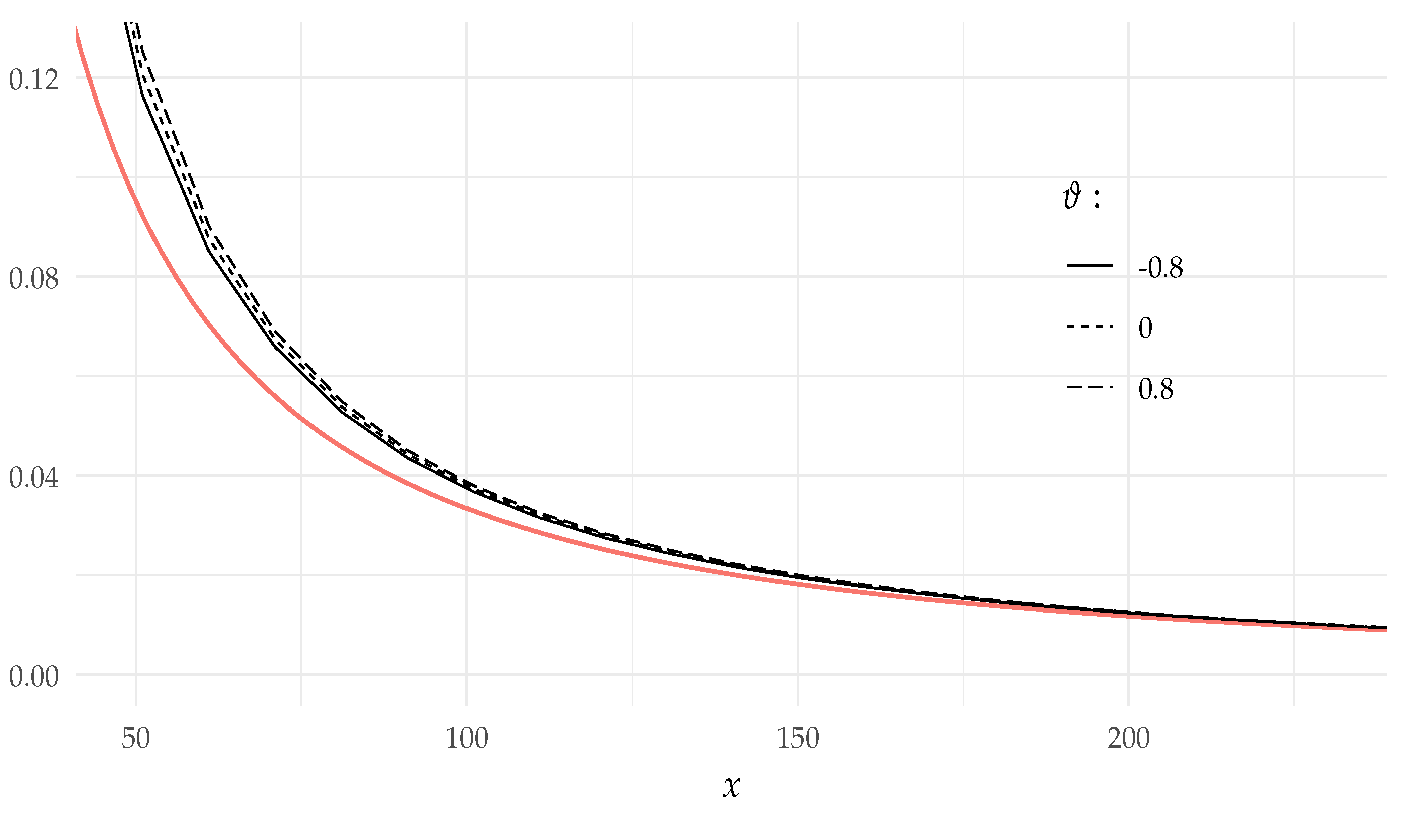
• Under the conditions of Example 3, we get from Theorem 3 that

  $$\mathbb{E}\left({({\xi }_1+{\xi }_2)}^{1/2}{\mathrm{𝕝}}_{\{{\xi }_1+{\xi }_2>x\}}\right)\sim \sum _{k=1}^2\mathbb{E}\left({\xi }_k^{1/2}{\mathrm{𝕝}}_{{\xi }_k>x}\right)\left[=\frac{100}{3x^{3/2}}\left(1+\frac{150}{7x^2}\right),x>5\right]$$

  for all $\vartheta \in \{-0.8,0,0.8\}$, according to the expressions of truncated moments derived in Section 6.2. The results of simulated values of $\mathbb{E}\left({({\xi }_1+{\xi }_2)}^{1/2}{\mathrm{𝕝}}_{\{{\xi }_1+{\xi }_2>x\}}\right)$ together with the values of the derived asymptotic formula are presented in Figure 1.
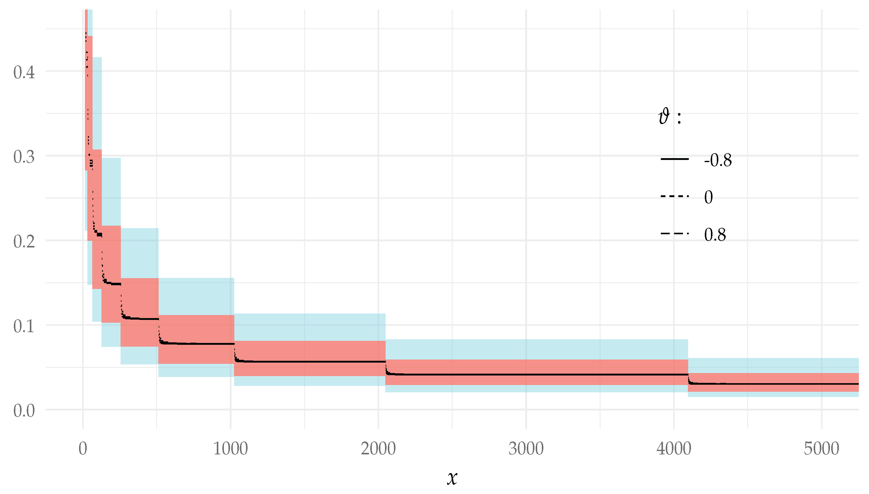
• The conditions of Example 4 and Theorem 3 imply that

  $$\begin{array}{cc}\hfill \mathbb{E}\left({({\xi }_1+{\xi }_2)}^{0.06}{\mathrm{𝕝}}_{\{{\xi }_1+{\xi }_2>x\}}\right)& \lesssim \sum _{k=1}^2\frac{1}{L_{{\xi }_k}}\mathbb{E}\left({\xi }_k^{0.06}{\mathrm{𝕝}}_{\{{\xi }_k>x\}}\right)\hfill \\ \hfill & \left[=\frac{2}{2^{0.94}-1}{2}^{-0.94\lfloor {log}_{2}x\rfloor }+\frac{2-\sqrt{2}}{2^{0.44}-1}{2}^{-0.44\lfloor {log}_{2}x\rfloor },x>1\right],\hfill \\ \hfill \mathbb{E}\left({({\xi }_1+{\xi }_2)}^{0.06}{\mathrm{𝕝}}_{\{{\xi }_1+{\xi }_2>x\}}\right)& \gtrsim \sum _{k=1}^2{L}_{{\xi }_k}\mathbb{E}\left({\xi }_k^{0.06}{\mathrm{𝕝}}_{\{{\xi }_k>x\}}\right)\hfill \\ \hfill & \left[=\frac{1}{2(2^{0.94}-1)}{2}^{-0.94\lfloor {log}_{2}x\rfloor }+\frac{(\sqrt{2}-1)}{\sqrt{2}(2^{0.44}-1)}{2}^{-0.44\lfloor {log}_{2}x\rfloor },x>1\right]\hfill \end{array}$$

  due to the formulas derived in Section 6.2. The results of the simulated values of $\mathbb{E}\left({({\xi }_1+{\xi }_2)}^{0.06}{\mathrm{𝕝}}_{\{{\xi }_1+{\xi }_2>x\}}\right)$ together with the asymptotic values are presented in Figure 2.
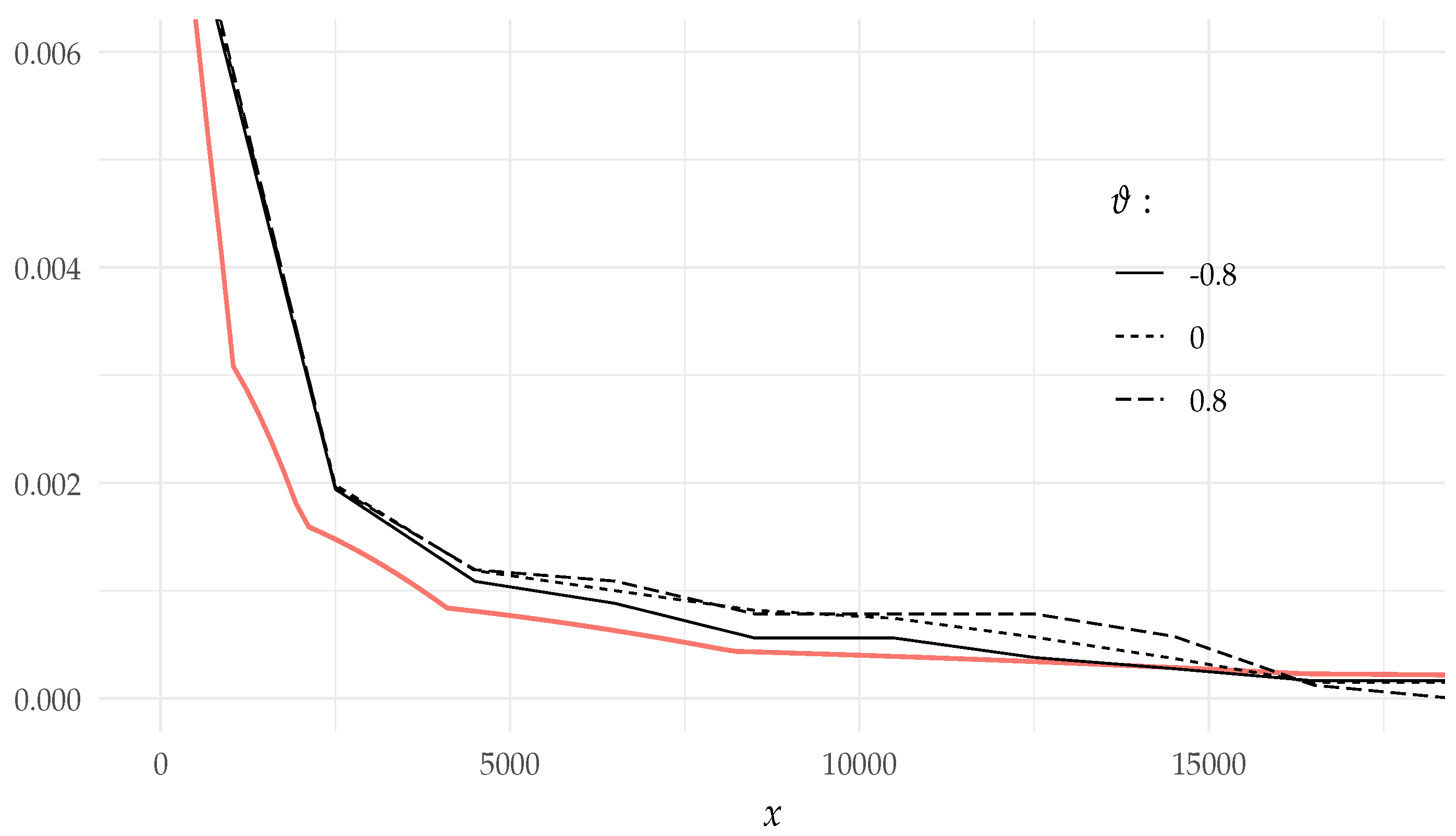
• Under the conditions of Example 5, Theorem 3 implies that $\mathbb{E}\left({({\xi }_1+{\xi }_2)}^{0.8}{\mathrm{𝕝}}_{\{{\xi }_1+{\xi }_2>x\}}\right)$ can be approximated by sum

  $$\begin{array}{cc}\hfill & \sum _{k=1}^2\mathbb{E}\left({\xi }_k^{0.8}{\mathrm{𝕝}}_{{\xi }_k>x}\right)=\frac{4}{9}\left({10}^{-\lfloor {log}_{2}x\rfloor }\left(2^{1.8\lceil {log}_{2}x\rceil }-x^{1.8}\right)+\frac{(2^{1.8}-1){(2^{4/5}/5)}^{\lceil {log}_{2}x\rceil }}{1-2^{4/5}/5}\right)\hfill \\ \hfill & +\frac{7}{18}\left[{\left(\frac{3}{10}\right)}^{\lfloor {log}_{2}x\rfloor }\left(2^{\lceil {log}_{2}x\rceil }-x^{1.8}\right)+\frac{(2^{1.8}-1){(2^{4/5}3/10)}^{\lceil {log}_{2}x\rceil }}{1-2^{4/5}3/10}\right],x>1,\hfill \end{array}$$

  for large x and for all three parameter $\vartheta$ values. The simulated values of $\mathbb{E}\left({({\xi }_1+{\xi }_2)}^{0.8}{\mathrm{𝕝}}_{\{{\xi }_1+{\xi }_2>x\}}\right)$ and its asymptotic values are presented in Figure 3.

From the presented graphs, we can see that the tail expectations $\mathbb{E}\left({({\xi }_1+{\xi }_2)}^{\alpha }{\mathrm{𝕝}}_{\{{\xi }_1+{\xi }_2>x\}}\right)$ are approximated quite accurately by their asymptotic values in all three examples. In addition, the effect of the copula dependence implied by the parameter $\vartheta$ quickly becomes negligible, as x attains larger values. In addition, we observe that the scale of the horizontal axis is different in each of the graphs, which reflects the different rate of convergence in the three examples.

To perform Monte Carlo simulations evaluating $\mathbb{E}\left({({\xi }_1+{\xi }_2)}^{\alpha }{\mathrm{𝕝}}_{\{{\xi }_1+{\xi }_2>x\}}\right)$ for each of the three examples, we firstly generated two samples consisting of $M=2\times {10}^7$ uniform random variates, namely vectors $(t_1,\dots ,t_M)$ and $(v_1,\dots ,v_M)$, and transformed them according to Algorithm $\mathcal{N}$ to induce the FGM copula dependence. Then, we modified each of the resulting vectors $(u_1,\dots ,u_M)$ and $(v_1,\dots ,v_M)$ according to the inverse probability integral transform described in Section 6.1, obtaining samples ${\left\{F_{{\xi }_1}^{\leftarrow }\left(u_k\right),F_{{\xi }_2}^{\leftarrow }\left(v_k\right)\right\}}_{k=1}^M$ from distributions $F_{{\xi }_1}$ and $F_{{\xi }_2}$. Finally, we replaced elements of the collection ${\left\{{(F_{{\xi }_1}^{\leftarrow }\left(u_k\right)+F_{{\xi }_2}^{\leftarrow }\left(v_k\right))}^{\alpha }\right\}}_{k=1}^M$ exceeding given threshold x by zeroes and calculated the empirical mean of the resulting vector.

All simulations were computed in the statistical programming package R [48]. Apart from the base R functions, several others from the tictoc [49], tikzDevice [50], furrr [51] and tidyverse [52] libraries were used.

7. Conclusions

In this paper, we investigate the asymptotic behaviour of tails of the moments for randomly weighted sums with possibly dependent dominatedly varying summands. Our results improve and generalise other related findings in the literature. Firstly, by putting the L-indices of individual summands inside the bounding sums, we achieve sharper asymptotic bounds under pQAI dependence structure. Moreover, we relax the condition for the exponent, allowing it to be any fixed nonnegative real number. Finally, in the case of randomly weighted sums, we substitute the boundedness condition on random weights by a less restrictive moments condition.

To illustrate and further validate the obtained results, we performed a Monte Carlo simulation study in which we considered three concrete examples of random sums from disjoint subclasses of dominatedly varying distributions. The simulations confirmed our derived asymptotic relations.

References

1. Chen, Y. A renewal shot noise process with subexponential shot marks. Risks 2019, 7, 63. [Google Scholar] [CrossRef] [Green Version]
2. Chen, Y.; Yuen, K.C. Sums of pairwise quasi-asymptotically independent random variables with consistent variation. Stoch. Models 2009, 25, 76–89. [Google Scholar] [CrossRef]
3. Cheng, D. Randomly weighted sums of dependent random variables with dominated variation. J. Math. Anal. Appl. 2014, 420, 1617–1633. [Google Scholar] [CrossRef]
4. Geluk, J.; Tang, Q. Asymptotic tail probabilities of sums of dependent subexponential random variables. J. Theoret. Probab. 2009, 22, 871–882. [Google Scholar] [CrossRef] [Green Version]
5. Goovaerts, M.J.; Kaas, R.; Laeven, R.J.A.; Tang, Q.; Vernic, R. The tail probability of discounted sums of Pareto-like losses in insurance. Scand. Actuar. J. 2005, 2005, 446–461. [Google Scholar] [CrossRef]
6. Jaunė, E.; Ragulina, O.; Šiaulys, J. Expectation of the truncated randomly weighted sums with dominatedly varying summands. Lith. Math. J. 2018, 58, 421–440. [Google Scholar] [CrossRef]
7. Leipus, R.; Šiaulys, J.; Vareikaitė, I. Tails of higher-order moments with dominatedly varying summands. Lith. Math. J. 2019, 59, 389–407. [Google Scholar] [CrossRef]
8. Tang, Q.; Tsitsiashvili, G. Precise estimates for the ruin probability in finite horizon in a discrete-time model with heavy-tailed insurance and financial risks. Stoch. Process. Appl. 2003, 108, 299–325. [Google Scholar] [CrossRef]
9. Wang, D.; Su, C.; Zeng, Y. Uniform estimate for maximum of randomly weighted sums with applications to insurance risk theory. Sci. China Ser. A 2005, 48, 1379–1394. [Google Scholar] [CrossRef]
10. Wang, D.; Tang, Q. Tail probabilities of randomly weighted sums of random variables with dominated variation. Stoch. Models 2006, 22, 253–272. [Google Scholar] [CrossRef]
11. Yi, L.; Chen, Y.; Su, C. Approximation of the tail probability of randomly weighted sums of dependent random variables with dominated variation. J. Math. Anal. Appl. 2011, 376, 365–372. [Google Scholar] [CrossRef] [Green Version]
12. Yang, Y.; Ignatavičiūtė, E.; Šiaulys, J. Conditional tail expectation of randomly weighted sums with heavy-tailed distributions. Stat. Probab. Lett. 2015, 105, 20–28. [Google Scholar] [CrossRef]
13. Fougeres, A.L.; Mercadier, C. Risk measures and multivariate extensions of Breiman’s theorem. J. Appl. Probab. 2012, 49, 364–384. [Google Scholar] [CrossRef] [Green Version]
14. Nyrhinen, H. On the ruin probabilities in a general economic environment. Stoch. Process. Appl. 1999, 83, 319–330. [Google Scholar] [CrossRef] [Green Version]
15. Tang, Q.; Yuan, Z. Randomly weighted sums of subexponential random variables with application to capital allocation. Extremes 2014, 17, 467–493. [Google Scholar] [CrossRef]
16. Wang, S.; Chen, C.; Wang, X. Some novel results on pairwise quasi-asymptotical independence with applications to risk theory. Comm. Stat. Theory Methods 2017, 46, 9075–9085. [Google Scholar] [CrossRef]
17. Verrall, R.J. The individual risk model: A compound distribution. J. Inst. Actuaries 1989, 116, 101–107. [Google Scholar] [CrossRef] [Green Version]
18. Dhaene, J.; Goovaerts, M.J. On the dependency of risks in the individual life model. Insur. Math. Econom. 1997, 19, 243–253. [Google Scholar] [CrossRef]
19. Dickson, D.C.M. Insurance Risk and Ruin; Cambridge University Press: Cambridge, UK, 2005. [Google Scholar]
20. Acerbi, C. Spectral measures of risks: A coherent representation of subjective risk aversion. J. Bank. Financ. 2002, 26, 1505–1518. [Google Scholar] [CrossRef] [Green Version]
21. Artzner, P.; Delbaen, F.; Eber, J.M.; Heath, D. Coherent measures of risk. Math. Financ. 1999, 9, 203–228. [Google Scholar] [CrossRef]
22. Asimit, A.V.; Furman, E.; Tang, Q.; Vernic, R. Asymptotics for risk capital allocations based on conditional tail expectation. Insur. Math. Econom. 2011, 49, 310–324. [Google Scholar] [CrossRef] [Green Version]
23. Hua, L.; Joe, H. Strength of tail dependence based on conditional tail expectation. J. Multivar. Anal. 2014, 123, 143–159. [Google Scholar] [CrossRef]
24. Wang, S.; Hu, Y.; Yang, L.; Wang, W. Randomly weighted sums under a wide type of dependence structure with application to conditional tail expectation. Commun. Stat. Theory Methods 2018, 47, 5054–5063. [Google Scholar] [CrossRef]
25. Goldie, C.M. Subexponential distributions and dominated-variation tails. J. Appl. Probab. 1978, 15, 440–442. [Google Scholar] [CrossRef]
26. Cai, J.; Tang, Q. On max-sum equivalence and convolution closure of heavy-tailed distributions and their applications. J. Appl. Probab. 2004, 41, 117–130. [Google Scholar] [CrossRef]
27. Cline, D.B.H.; Samorodnitsky, G. Subexponentiality of the product of independent random variables. Stoch. Process. Appl. 1994, 49, 75–98. [Google Scholar] [CrossRef] [Green Version]
28. Embrechts, P.; Goldie, C.M. On closure and factorization properties of subexponential and related distributions. J. Austral. Math. Soc. Ser. A 1980, 29, 243–256. [Google Scholar] [CrossRef] [Green Version]
29. Embrechts, P.; Omey, E. A property of longtailed distributions. J. Appl. Probab. 1984, 21, 80–87. [Google Scholar] [CrossRef]
30. Foss, S.; Korshunov, D.; Zachary, S. An Introduction to Heavy-Tailed and Subexponential Distributions, 2nd ed.; Springer: New York, NY, USA, 2013. [Google Scholar]
31. Konstantinides, D.G. Risk Theory. A Heavy Tail Approach; World Scientific Publishing: Singapore, 2018. [Google Scholar]
32. Pitman, E.J.G. Subexponential distribution functions. J. Austral. Math. Soc. Ser. A 1980, 29, 337–347. [Google Scholar] [CrossRef]
33. Wang, Y.B.; Wang, K.Y.; Cheng, D.Y. Precise large deviations for sums of negatively associated random variables with common dominatedly varying tails. Acta Math. Sin. (Engl. Ser.) 2006, 22, 1725–1734. [Google Scholar] [CrossRef]
34. Yang, Y.; Wang, Y. Asymptotics for ruin probability of some negatively dependent risk models with a constant interest rate and dominatedly-varying-tailed claims. Statist. Probab. Lett. 2010, 80, 143–154. [Google Scholar] [CrossRef]
35. Matuszewska, W. On a generalization of regularly increasing functions. Studia Math. 1964, 24, 271–279. [Google Scholar] [CrossRef] [Green Version]
36. Bingham, N.H.; Goldie, C.M.; Teugels, J.L. Regular Variation; Cambridge University Press: Cambridge, UK, 1987. [Google Scholar]
37. Sklar, M. Fonctions de répartition à n dimensions et leurs marges. Publ. Inst. Stat. Univ. Paris 1959, 8, 229–231. [Google Scholar]
38. Nelsen, R.B. An introduction to Copulas, 2nd ed.; Springer: New York, NY, USA, 2006. [Google Scholar]
39. Kotz, S.; Balakrishnan, N.; Johnson, N.L. Continuous Multivariate Distributions, 2nd ed.; John Wiley and Sons: New York, NY, USA, 2000; Volume 1. [Google Scholar]
40. Ali, M.M.; Mikhail, N.N.; Haq, M.S. A class of bivariate distributions including the bivariate logistic. J. Multivar. Anal. 1978, 8, 405–412. [Google Scholar] [CrossRef] [Green Version]
41. Albrecher, H.; Asmussen, S.; Kortschak, D. Tail asymptotics for the sum of two heavy-tailed dependent risks. Extremes 2006, 9, 107–130. [Google Scholar] [CrossRef]
42. Fang, H.; Ding, S.; Li, X.; Yang, W. Asymptotic approximations of ratio moments based on dependent sequences. Mathematics 2020, 8, 361. [Google Scholar] [CrossRef] [Green Version]
43. Yang, H.; Gao, W.; Li, J. Asymptotic ruin probabilities for a discrete-time risk model with dependent insurance and financial risks. Scand. Actuar. J. 2016, 2016, 1–17. [Google Scholar] [CrossRef]
44. Li, J. On pairwise quasi-asymptotically independent random variables and their applications. Stat. Probab. Lett. 2013, 83, 2081–2087. [Google Scholar] [CrossRef]
45. Embrechts, P.; Hofert, M. A note on generalized inverses. Math. Methods Oper. Res. (Heidelb) 2013, 77, 423–432. [Google Scholar] [CrossRef] [Green Version]
46. Rosenblatt, M. Remarks on a multivariate transformation. Ann. Math. Stat. 1952, 23, 470–472. [Google Scholar] [CrossRef]
47. Brockwell, A.E. Universal residuals: A multivariate transformation. Stat. Probab. Lett. 2007, 77, 1473–1478. [Google Scholar] [CrossRef] [PubMed] [Green Version]
48. R Core Team. R: A Language and Environment for Statistical Computing; R Foundation for Statistical Computing: Vienna, Austria, 2018; Available online: https://www.R-project.org/ (accessed on 15 December 2020).
49. Izrailev, S. Tictoc: Functions for Timing R Scripts, as Well as Implementations of Stack and List Structures. R Package Version 1.0. 2014. Available online: https://CRAN.R-project.org/package=tictoc (accessed on 23 December 2020).
50. Sharpsteen, C.; Bracken, C. tikzDevice: R Graphics Output in LaTeX Format. R Package Version 0.12.3.1. 2020. Available online: https://CRAN.R-project.org/package=tikzDevice (accessed on 9 January 2021).
51. Vaughan, D.; Dancho, M. Furrr: Apply Mapping Functions in Parallel Using Futures. R Package Version 0.1.0. 2018. Available online: https://CRAN.R-project.org/package=furrr (accessed on 17 January 2021).
52. Wickham, H.; Averick, M.; Bryan, J.; Chang, W.; McGowan, L.D.; François, R.; Grolemund, G.; Hayes, A.; Henry, L.; Hester, J.; et al. Welcome to the tidyverse. J. Open Source Softw. 2019, 4, 1686. [Google Scholar] [CrossRef]
Figure 1. Simulated and asymptotic values for the truncated expectation of Example 3. Solid red line represents the exact asymptotic values of k = 1 2 E ξ k 1 / 2 𝕝 { ξ k > x } .
Mathematics 09 00824 g001
Figure 2. Simulated and asymptotic values for the truncated expectation of Example 4. Red area represents the region bounded by k = 1 2 L ξ k E ξ k 0.06 𝕝 { ξ k > x } and k = 1 2 L ξ k 1 E ξ k 0.06 𝕝 { ξ k > x } . Cyan area reflects the additional error using bounding coefficients L 2 ξ = min { L ξ 1 , L ξ 2 } and ( L 2 ξ ) 1 .
Mathematics 09 00824 g002
Figure 3. Simulated and asymptotic values for the truncated expectation of Example 5. Solid red line represents the exact asymptotic values of k = 1 2 E ξ k 0.8 𝕝 { ξ k > x } .
Mathematics 09 00824 g003
Publisher’s Note: MDPI stays neutral with regard to jurisdictional claims in published maps and institutional affiliations.