Stability of Systems of Fractional-Order Differential Equations with Caputo Derivatives

Abstract

Systems of fractional-order differential equations present stability properties which differ in a substantial way from those of systems of integer order. In this paper, a detailed analysis of the stability of linear systems of fractional differential equations with Caputo derivative is proposed. Starting from the well-known Matignon’s results on stability of single-order systems, for which a different proof is provided together with a clarification of a limit case, the investigation is moved towards multi-order systems as well. Due to the key role of the Mittag–Leffler function played in representing the solution of linear systems of FDEs, a detailed analysis of the asymptotic behavior of this function and of its derivatives is also proposed. Some numerical experiments are presented to illustrate the main results.

1. Introduction

The investigation of stability properties plays a prominent role in the qualitative theory of fractional-order systems, similarly as in the case of the classical theory of integer-order dynamical systems [1,2]. The classical Hartman–Grobman linearisation theorem, which states that the local behavior of a dynamical system in a neighborhood of a hyperbolic equilibrium is qualitatively equivalent to the behavior of its linearisation near the equilibrium, is extended to the case of fractional-order systems as well [3,4,5]. Consequently, linear stability analysis is of fundamental importance in the investigation of fractional-order systems, and, in particular, stability properties of linear autonomous systems of fractional-order differential equations play a key role in this context.

For single-order systems of fractional differential equations (FDEs), namely systems in which the FDEs have the same fractional order, the most important theoretical result, which may now be considered classical, is Matignon’s stability theorem [6], recently generalized in [7] for the case when the fractional order belongs to the interval $(0,2)$.

Thus far, the investigation of stability properties of multi-order (incommensurate) fractional-order systems has unquestionably received less consideration. We refer to [8,9,10,11] for the stability analysis of incommensurate fractional-order systems with rational orders. Moreover, closely linked to this research topic, bounded input bounded output stability of systems with irrational transfer functions has been investigated in [12,13]. Very recently, the asymptotic properties of solutions of several classes of linear multi-order systems of fractional differential equations (such as systems with block triangular coefficient matrices) have been considered in [14].

The main difficulty in establishing necessary and sufficient conditions for the stability of multi-order linear systems of fractional differential equations (conceivably comparable to the classical Routh–Hurwitz conditions for integer-order systems) is due to the fact that a large number of parameters are involved: the system’s coefficients, as well as multiple fractional orders. Undoubtedly, the complexity of the problem is positively correlated with the system’s dimension.

The case of two-dimensional multi-order fractional-order systems has been fully investigated in [15,16,17]. On one hand, necessary and sufficient conditions for the asymptotic stability and instability of the fractional-order system have been obtained, in terms of the main diagonal elements and the determinant of the system’s matrix, as well as the fractional orders of the Caputo derivatives. Moreover, necessary and sufficient fractional-order independent conditions have also been presented, in terms of the main diagonal elements and the determinant of the system’s matrix, which guarantee the asymptotic stability or instability of the considered two-dimensional system, regardless of the choice of the fractional-orders considered in the system. These latter results prove to be especially useful in practical applications where the exact fractional orders of the Caputo derivatives are not precisely known.

It is important to note that multi-term fractional-order differential equations [18] and their qualitative properties are sharply linked to multi-order systems of fractional differential equations. We refer to [11] for a thorough presentation of the relationship between these two concepts. The investigation of stability properties of multi-term FDEs is so far limited to two-term and three-term fractional-order differential and difference equations, which have been recently studied in [19,20,21,22]. However, due to the increasing complexity of the problem, equations with four or more fractional terms have not yet been investigated.

This paper is organized as follows: Section 2 illustrates the statement of the problem and the main definitions. Due to the importance in the description of the solution of linear systems of FDEs, in Section 3, we provide a detailed description of the Mittag–Leffler function, of its derivatives and of the corresponding asymptotic behavior. Section 4 investigates the stability properties of single-order systems of FDEs, by presenting classical Matignon’s theorem and some simulations illustrating the different stability behavior in dependence of the spectral properties of the matrix system. Stability analysis of multi-order systems is discussed in Section 5; since general results are far from being formulated in this case, we focus on some special cases and we separately investigate two-dimensional systems, higher dimensional systems with block-triangular structure, and higher dimensional systems with some special fractional orders. Some concluding remarks are hence provided in the concluding Section 6.

2. Preliminaries

Consider an n-dimensional fractional-order system with Caputo derivatives:

$${}^{\mathrm{C}}{D}^{\mathbf{q}}\mathbf{y}\left(t\right)=f(t,\mathbf{y})$$

(1)

with $\mathbf{q}=(q_1,q_2,...,q_n)\in {(0,1]}^n$, assuming that $f:[0,\infty )\times {\mathbb{R}}^n\to {\mathbb{R}}^n$ is a continuous function on its domain of definition, Lipschitz-continuous with respect to the second variable and $\mathbf{y}:[0,\infty )\to {\mathbb{R}}^n$ a vector-valued function. With ${}^{\mathrm{C}}{D}^{\mathbf{q}}\mathbf{y}\left(t\right)$, we denote the application of the Caputo derivative of order $0<q_i\le 1$ to each component $y_i\left(t\right)$ of $\mathbf{y}\left(t\right)$, namely

$${}^{\mathrm{C}}{D}^{\mathbf{q}}\mathbf{y}\left(t\right)=\left(\begin{array}{c}{}^{\mathrm{C}}{D}^{q_1}{y}_1\left(t\right)\\ {}^{\mathrm{C}}{D}^{q_2}{y}_2\left(t\right)\\ ⋮\\ {}^{\mathrm{C}}{D}^{q_n}{y}_n\left(t\right)\end{array}\right),{}^{\mathrm{C}}{D}^{q_i}{y}_i\left(t\right)\frac{1}{\mathrm{\Gamma }(1-q_i)}{\int }_0^t{(t-\mathrm{\tau })}^{-q_i}{y}_i^{\prime }\left(\mathrm{\tau }\right)\mathrm{d}\tau .$$

Existence and uniqueness of the solution of initial value problems associated with system (1) is ensured by Corollary 2.4 from [14].

Whenever $q_1=q_2=\dots =q_n$, system (1) is said to be single-order; otherwise, the term multi-order will be used.

Let us further assume that $\mathbf{y}=0$ is an equilibrium solution of system (1), i.e.,

$$f(t,0)=0\mathrm{for}\mathrm{any}t\ge 0.$$

Definition 1.

Let $\alpha >0$ and denote by $\phi (t,{\mathbf{y}}_0)$ the unique solution of (1) satisfying the initial condition $\mathbf{y}\left(0\right)={\mathbf{y}}_0\in {\mathbb{R}}^n$. Then:

i. 

 the trivial solution of (1) is called stable if for any $\epsilon >0$ there exists $\delta =\delta \left(\epsilon \right)>0$ such that, for every ${\mathbf{y}}_0\in {\mathbb{R}}^n$ satisfying $\parallel {\mathbf{y}}_0\parallel <\delta$, we have $\parallel \phi (t,{\mathbf{y}}_0)\parallel \le \epsilon$ for any $t\ge 0$;

ii. 

 the trivial solution of (1) is called asymptotically stable if it is stable and there exists $\rho >0$ such that $\underset{t\to \infty }{lim}\phi (t,{\mathbf{y}}_0)=0$ for $\parallel {\mathbf{y}}_0\parallel <\rho$;

iii. 

 the trivial solution of (1) is called $\mathcal{O}\left(t^{-\alpha }\right)$-asymptotically stable if it is stable and there exists $\rho >0$ such that, for any $\parallel {\mathbf{y}}_0\parallel <\rho$, we have:

$$\parallel \phi (t,{\mathbf{y}}_0)\parallel =\mathcal{O}\left(t^{-\alpha }\right)as t\to \infty .$$

Remark 1.

In the particular case of linear systems of fractional-order differential equations with constant coefficients, we say that the system is stable/asymptotically stable/unstable if and only if its trivial solution is stable/asymptotically stable/unstable.

3. Mittag–Leffler Functions, Derivatives and Asymptotic Behavior

In the analysis of linear systems of FDEs, a crucial role is played by the Mittag–Leffler (ML) function [23]

$$E_{\alpha ,\beta }\left(z\right)=\sum _{k=0}^{\infty }\frac{z^k}{\mathrm{\Gamma }(\alpha k+\beta )},\alpha >0,z\in \mathbb{C},$$

(2)

where $\mathrm{\Gamma }\left(x\right)={\int }_0^{\infty }{t}^{x-1}{\mathrm{e}}^{-t}\mathrm{d}t$ is the Euler–Gamma function. Since $\mathrm{\Gamma }(k+1)=k!$, $k\in \mathbb{N}$, this function generalizes the exponential function when $\alpha =\beta =1$, namely $E_{1,1}\left(z\right)={\mathrm{e}}^z$. When $\beta =1$, the notation $E_{\alpha }\left(z\right)E_{\alpha ,1}\left(z\right)$ is preferred.

For the purposes of this paper (the reasons will be clearer later on), it is convenient to study and introduce a further generalization of the ML function.

3.1. The Prabhakar Function and Its Asymptotic Properties

For three real parameters $\alpha$, $\beta$ and $\gamma$, the three-parameter Mittag–Leffler (ML) function, also known as the Prabhakar function [24], is defined by its series representation

$$E_{\alpha ,\beta }^{\gamma }\left(z\right)=\frac{1}{\mathrm{\Gamma }\left(\gamma \right)}\sum _{k=0}^{\infty }\frac{\mathrm{\Gamma }(\gamma +k)z^k}{kj!\mathrm{\Gamma }(\alpha k+\beta )},\alpha >0,z\in \mathbb{C}.$$

This function is not only a generalization, to three parameters, of the two-parameter ML function $E_{\alpha ,\beta }\left(z\right)$ (indeed, when $\gamma =1$, it is $E_{\alpha ,\beta }^1\left(z\right)=E_{\alpha ,\beta }\left(z\right)$), but it also provides a simple and elegant way to represent derivatives of two-parameter ML functions since

$$E_{\alpha ,\beta }^{\left(m\right)}\left(z\right)\frac{{\mathrm{d}}^m}{\mathrm{d}{z}^m}{E}_{\alpha ,\beta }\left(z\right)=m!E_{\alpha ,\alpha m+\beta }^{m+1}\left(z\right),m=0,1,2,\cdots ,$$

(3)

as one can easily check after a term-by-term differentiation of (2).

In order to introduce a result about the Laplace transform (LT), it is necessary to introduce what is known as the Prabhakar kernel

$$e_{\alpha ,\beta }^{\gamma }(t;\lambda )=t^{\beta -1}{E}_{\alpha ,\beta }^{\gamma }\left(t^{\alpha }\lambda \right),t>0,\lambda \in \mathbb{C},$$

for which the following analytical representation of the LT is available:

$${\mathcal{E}}_{\alpha ,\beta }^{\gamma }(s;\lambda ):=\mathcal{L}\left[e_{\alpha ,\beta }^{\gamma }(t;\lambda );s\right]=\frac{s^{\alpha \gamma -\beta }}{{(s^{\alpha }-\lambda )}^{\gamma }}{,\Re \left(s\right)>0,\left|s\right|>\left|\lambda \right|}^{\frac{1}{\alpha }}.$$

Having in mind the stability analysis of linear FDEs, whose solutions will be expressed in terms of Mittag–Leffler functions and their derivatives, it is of interest to recall some results about the asymptotic behavior of the Prabhakar function in the complex plane.

In particular, for large arguments and $0<\alpha \le 1$, we first identify exponential and algebraic expansions, respectively given by

$$\begin{array}{cc}\hfill {\mathcal{F}}_{\alpha ,\beta }^{\gamma }\left(z\right)& =\frac{1}{\mathrm{\Gamma }\left(\gamma \right)}{\mathrm{e}}^{z^{1/\alpha }}{z}^{\frac{\gamma -\beta }{\alpha }}\frac{1}{{\alpha }^{\gamma }}\sum _{j=0}^{\infty }{c}_j{z}^{-\frac{j}{\alpha }}\hfill \\ \hfill {\mathcal{A}}_{\alpha ,\beta }^{\gamma }\left(z\right)& =\frac{z^{-\gamma }}{\mathrm{\Gamma }\left(\gamma \right)}\sum _{j=0}^{\infty }\frac{{(-1)}^j\mathrm{\Gamma }(j+\gamma )}{j!\mathrm{\Gamma }(\beta -\alpha (j+\gamma \left)\right)}{z}^{-j},\hfill \end{array}$$

and, thanks to the results obtained by Paris [25,26], we know that

$$E_{\alpha ,\beta }^{\gamma }\left(z\right)\sim \left\{\begin{array}{cc}{\mathcal{F}}_{\alpha ,\beta }^{\gamma }\left(z\right)+{\mathcal{A}}_{\alpha ,\beta }^{\gamma }\left(z{\mathrm{e}}^{\mp \pi \mathrm{i}}\right)\hfill & |argz|<\frac{\alpha \pi }{2}\hfill \\ {\mathcal{A}}_{\alpha ,\beta }^{\gamma }\left(z{\mathrm{e}}^{\mp \pi \mathrm{i}}\right)+{\mathcal{F}}_{\alpha ,\beta }^{\gamma }\left(z\right)\hfill & \frac{\alpha \pi }{2}<|argz|<\alpha \pi \hfill \\ {\mathcal{A}}_{\alpha ,\beta }^{\gamma }\left(z{\mathrm{e}}^{\mp \pi \mathrm{i}}\right)\hfill & \alpha \pi <|argz|\le \pi \hfill \end{array}\right.,\left|z\right|\to \infty$$

with the sign in ${\mathrm{e}}^{\mp \pi \mathrm{i}}$ which must taken negative for z in the upper complex half-plane and positive otherwise. Following the convention adopted in [27], in each sum, we have first indicated the dominant term, namely the exponential term ${\mathcal{F}}_{\alpha ,\beta }^{\gamma }\left(z\right)$ when $|argz|<\frac{\alpha \pi }{2}$ and the algebraic term ${\mathcal{A}}_{\alpha ,\beta }^{\gamma }\left(z{\mathrm{e}}^{\mp \pi \mathrm{i}}\right)$ when $\frac{\alpha \pi }{2}<|argz|<\alpha \pi$. The lines $|argz|=\alpha \pi$ and $|argz|=\frac{\alpha \pi }{2}$ are, respectively, Stokes and anti-Stokes lines where asymptotic expansions change their behavior. The above result is graphically summarized in Figure 1.

We first recall that coefficients $c_j$ in asymptotic expansion ${\mathcal{F}}_{\alpha ,\beta }^{\gamma }\left(z\right)$ are obtained [25] from the inverse factorial expansion, for $\left|s\right|\to \infty$ in $|arg(s\left)\right|\le \pi -ϵ$ and any arbitrarily small $ϵ>0$, of

$$F_{\alpha ,\beta }^{\gamma }\left(s\right):=\frac{\mathrm{\Gamma }(\gamma +s)\mathrm{\Gamma }(\alpha s+\psi )}{\mathrm{\Gamma }(s+1)\mathrm{\Gamma }(\alpha s+\beta )}={\alpha }^{1-\gamma }\left(1+\sum _{j=1}^{\infty }\frac{c_j}{{(\alpha s+\psi )}_j}\right)$$

(4)

with ${\left(x\right)}_j=\mathrm{\Gamma }(x+j)/\mathrm{\Gamma }\left(x\right)$ the Pochhammer symbol and $\psi =1-\gamma +\beta$. They can be evaluated by means of a sophisticated algorithm introduced in in [25] and also explained in [28]. The first few entries of $c_k$ are available in [26].

Based on the asymptotic properties of the Prabhakar function, we obtain the asymptotic equivalence:

$$e_{\alpha ,\beta }^{\gamma }(t;\lambda )\sim \left\{\begin{array}{cc}{\displaystyle \frac{{\lambda }^{\frac{\gamma -\beta }{\alpha }}}{\mathrm{\Gamma }\left(\gamma \right)}}{t}^{\gamma -1}{\mathrm{e}}^{t{\lambda }^{1/\alpha }}\hfill & \mathrm{if}|arg\left(\lambda \right)|\le \frac{\alpha \pi }{2}\hfill \\ {\displaystyle \frac{{\mathrm{e}}^{\pm \gamma \pi \mathrm{i}}}{{\lambda }^{\gamma }\mathrm{\Gamma }(\beta -\alpha \gamma )}}{t}^{\beta -\alpha \gamma -1}\hfill & \mathrm{if}|arg\left(\lambda \right)|>\frac{\alpha \pi }{2}\hfill \end{array}\right.$$

(5)

as $t\to \infty$, where the sign in the term ${\mathrm{e}}^{\pm \gamma \pi \mathrm{i}}$ is positive if $\lambda$ is in the upper complex half-plane, and negative otherwise.

3.2. Asymptotic Behavior of Derivatives of the ML Function

Thanks to the relationship (3) between derivatives of the ML function and the Prabhakar function, the investigation of the asymptotic behavior of any m-th order derivative of $E_{\alpha ,\beta }\left(z\right)$ is hence possible by applying the corresponding results for the Prabhakar function and afterwards replacing $\beta$ with $\alpha m+\beta$ and $\gamma$ with $m+1$.

To this purpose, we first observe that, after these replacements, the function $F_{\alpha ,\beta }^{\gamma }\left(s\right)$ in (4) becomes $F_{\alpha ,\alpha m+\beta }^{m+1}\left(s\right)={(s+1)}_m/{(\alpha s+\psi )}_m$, with $\psi =\alpha m+\beta$. Hence, coefficients $c_j$ vanish for $j=m+1,m+2,\cdots$ and the exponential and algebraic expansions read

$$\begin{array}{cc}\hfill {\mathcal{F}}_{\alpha ,\alpha m+\beta }^{m+1}\left(z\right)& =\frac{1}{m!}{\mathrm{e}}^{z^{1/\alpha }}{z}^{\frac{1-\alpha m-\beta }{\alpha }}\frac{1}{{\alpha }^{m+1}}\sum _{j=0}^m{c}_j{z}^{\frac{m-j}{\alpha }}\hfill \\ \hfill {\mathcal{A}}_{\alpha ,\alpha m+\beta }^{m+1}\left(z\right)& =\frac{1}{m!}\sum _{j=0}^{\infty }\frac{{(-1)}^j{(j+1)}_m}{\mathrm{\Gamma }(\beta -\alpha (j+1\left)\right)}{z}^{-j-m-1},\hfill \end{array}$$

Therefore, by taking into account just the dominant expansions in each sector of the complex plane delimited by Stokes and anti-Stokes lines, and just leading terms in each expansion, we can describe the asymptotic behavior of derivatives of the ML function as

$$\frac{{\mathrm{d}}^m}{\mathrm{d}{z}^m}{E}_{\alpha ,\beta }\left(z\right)\sim \left\{\begin{array}{cc}{\displaystyle \frac{1}{{\alpha }^{m+1}}{\mathrm{e}}^{z^{1/\alpha }}{z}^{\frac{m+1-\alpha m-\beta }{\alpha }}}\hfill & |argz|<\frac{\alpha \pi }{2}\hfill \\ {\displaystyle {(-1)}^{m+1}\frac{m!}{\mathrm{\Gamma }(\beta -1)}{z}^{-m-1}}\hfill & \alpha \pi <|argz|\le \pi \hfill \end{array}\right.,\left|z\right|\to \infty$$

3.3. Behavior of Derivatives of the ML Function When $|argz|=\frac{\alpha \pi }{2}$

It remains to investigate the behavior along the anti-Stokes line $|argz|=\frac{\alpha \pi }{2}$ where both the exponential and the algebraic terms are present. We therefore consider

$$z=\rho {\mathrm{e}}^{\pm \frac{\alpha \pi }{2}\mathrm{i}},\rho >0$$

and, for large $\rho =\left|z\right|$, it is

$$\begin{array}{cc}\hfill \frac{{\mathrm{d}}^m}{\mathrm{d}{z}^m}{E}_{\alpha ,\beta }\left(z\right)\sim & {\mathrm{e}}^{\pm \mathrm{i}{\rho }^{1/\alpha }}\frac{1}{{\alpha }^{m+1}}\sum _{j=0}^m{c}_j{\rho }^{\frac{1-\alpha m-\beta +m-j}{\alpha }}{\mathrm{e}}^{\pm (1-\alpha m-\beta +m-j)\frac{\pi }{2}\mathrm{i}}+\hfill \\ & +\sum _{j=0}^{\infty }\frac{{(-1)}^j{(j+1)}_m}{\mathrm{\Gamma }(\beta -\alpha (j+1\left)\right)}\frac{1}{{\rho }^{m+1+j}}{\mathrm{e}}^{-\mathrm{i}(m+1+j)(\frac{\alpha }{2}-1)\pi }.\hfill \end{array}$$

Clearly, the second term asymptotically goes to zero when $\rho \to \infty$. The first term, instead, in modulus asymptotically tends to zero only for suitable values of $\alpha$ and $\beta$ such that $1-\alpha m-\beta +m-j\le 0$ for any $j\in \{0,1,\cdots ,m\}$, namely, when $1-\alpha m-\beta +m\le 0$ or, equivalently, when

$$m\le \frac{\beta -1}{1-\alpha }.$$

When we consider the one-parameter ML function $E_{\alpha }\left(z\right)$, namely $\beta =1$, which is the instance of the ML involved in the stability analysis of linear FDEs, for $argz=\pm \frac{\alpha \pi }{2}$ just $\left|E_{\alpha }\left(z\right)\right|$ asymptotically converges to $1/\alpha$ for $\left|z\right|\to \infty$ but any m-th order derivative of $E_{\alpha }\left(z\right)$, with $m\ge 0$, is unbounded when $\left|z\right|\to \infty$.

This situation is illustrated in Figure 2, where we report the first derivatives of $E_{\alpha }\left(z\right)$ for $\alpha =0.6$ and $\alpha =0.8$ evaluated for z along the anti-Stokes line $argz=\frac{\alpha \pi }{2}$ (results are similar when $argz=-\frac{\alpha \pi }{2}$).

Remark 2.

The behavior on the anti-Stokes line $|argz|=\frac{\alpha \pi }{2}$ of m-th order derivatives of the ML function $E_{\alpha }\left(z\right)$, which are unbounded as $\left|z\right|\to \infty$ for $m\ge 1$, is quite different from that of the exponential function ${\mathrm{e}}^z$ (namely, the special instance of $E_{\alpha }\left(z\right)$ for $\alpha =1$). Indeed, derivatives of the the exponential are never unbounded on the corresponding anti-Stokes lines $|argz|=\frac{\pi }{2}$ since there it is $\left|{\mathrm{d}}^m/\mathrm{d}{z}^m{\mathrm{e}}^z\right|=1$ for any $m=0,1,\cdots$

4. Stability of Linear Systems of Single-Order FDEs

We first consider the following linear system of Caputo-type fractional-order differential equations of the same fractional order:

$${}^{\mathrm{C}}{D}^{q}y\left(t\right)=Ay\left(t\right),$$

(6)

where $q\in (0,1]$ and $A\in {\mathbb{R}}^{n\times n}$, coupled with the initial condition $y\left(0\right)=y_0\in {\mathbb{R}}^n$.

In is important to emphasize that system (6) is equivalent to the following system of weakly singular Volterra integral equations of convolution type (see, for example, [29,30]):

$$y\left(t\right)=y_0+A{\int }_0^t\frac{{(t-\mathrm{\tau })}^{q-1}}{\mathrm{\Gamma }\left(q\right)}y\left(\mathrm{\tau }\right)\mathrm{d}\mathrm{\tau }.$$

(7)

For the most important advances regarding the general theory of linear Volterra integral equations, including the case when the convolution kernel is completely monotonic, we refer to [31,32,33,34].

The characteristic equation associated with system (6) is

$$det\left(s^{q}I-A\right)=0,$$

(8)

where, according to [35], the principal value (first branch) of the complex power function is considered. Therefore, it is easy to see that s is a root of the characteristic Equation (8) if and only if there exists an eigenvalue $\lambda$ of the matrix A such that

$$s^q=\lambda .$$

(9)

Hence, this leads to the following characterization of the stability properties of system (6), in terms of the roots of its characteristic equation:

Proposition 1.

The linear system (6) is asymptotically stable if and only if

$$\sigma \left(A\right)\subset S_q$$

where $\sigma \left(A\right)$ denotes the spectrum of the matrix A and

$$S_q=\{\lambda \in \mathbb{C}:s^q\ne \lambda ,\forall \Re \left(s\right)\ge 0\}.$$

With the aim of investigating the stability properties of system (6) by characterizing the stability region $S_q$, and presenting a concise proof of Matignon’s theorem [6], it is convenient to use the Jordan normal form of the matrix A. Indeed, let us consider a nonsingular matrix $P\in {\mathbb{C}}^{n\times n}$ such that

$$A=PJ{P}^{-1},J=\left(\begin{array}{cccc}{J}_1& 0& \dots & 0\\ 0& J_2& \dots & 0\\ ⋮& ⋮& \ddots & ⋮\\ 0& 0& \dots & J_p\end{array}\right)$$

where $J_k$, $k=1,\cdots ,p$ are Jordan blocks

$$J_k=\left(\begin{array}{cccccc}{\lambda }_k& 1& 0& \dots & 0& 0\\ 0& {\lambda }_k& 1& \dots & 0& 0\\ ⋮& \ddots & \ddots & \ddots & \ddots & ⋮\\ 0& 0& 0& \dots & {\lambda }_k& 1\\ 0& 0& 0& \dots & 0& {\lambda }_k\end{array}\right)$$

and ${\lambda }_k$ are eigenvalues of the matrix A. The size of the largest Jordan block $J_k$ of A associated with the eigenvalue ${\lambda }_k$ is called the index of ${\lambda }_k$ [36]. On the other hand, the total number of Jordan blocks associated with a given eigenvalue ${\lambda }_k$ in the Jordan normal form of the matrix A is the geometric multiplicity of the eigenvalue ${\lambda }_k$. Moreover, the sum of the sizes of all Jordan blocks corresponding to ${\lambda }_k$ is the algebraic multiplicity of ${\lambda }_k$. Therefore, the index of an eigenvalue ${\lambda }_k$ is equal to 1 if and only if its algebraic and geometric multiplicities are equal.

With these observations, we next give a slightly modified version of the classical result of Matignon, to fix a small imprecision in the second statement, related to the use of the geometric multiplicity instead of the index of an eigenvalue:

Theorem 1

(Matignon, 1996 [6]). The linear system (6) is

i. 

 $\mathcal{O}\left(t^{-q}\right)$-asymptotically stable if and only if

$$\sigma \left(A\right)\subset S_q=\left\{\lambda \in \mathbb{C}:|arg\left(\lambda \right)|>\frac{q\pi }{2}\right\}.$$

ii. 

 stable if and only if $\sigma \left(A\right)\subset \overline{S_q}$ and the eigenvalues of A which satisfy $|arg\left(\lambda \right)|={\displaystyle \frac{q\pi }{2}}$ have index 1.

Proof. 

With the notations introduced previously, denoting $z\left(t\right)=Py\left(t\right)$, it is easy to verify that system (6) is equivalent to

$${}^{\mathrm{C}}{D}^{q}z\left(t\right)=Jz\left(t\right).$$

(10)

Applying the LT to the linear system (10) leads to the following formula for the LT of the vector function $z\left(t\right)$:

$$Z\left(s\right)=s^{q-1}{(s^{q}I-J)}^{-1}z\left(0\right)$$

(11)

Since the Jordan normal form J is a block diagonal matrix, the matrix ${(s^{q}I-J)}^{-1}$ is also block diagonal, and its blocks are upper triangular matrices of the form:

$${(s^{q}I-J_k)}^{-1}=\left(\begin{array}{cccc}{(s^q-{\lambda }_k)}^{-1}& {(s^q-{\lambda }_k)}^{-2}& \dots & {(s^q-{\lambda }_k)}^{-d_k}\\ 0& {(s^q-{\lambda }_k)}^{-1}& \dots & {(s^q-{\lambda }_k)}^{-(d_k-1)}\\ ⋮& ⋮& \ddots & ⋮\\ 0& 0& \dots & {(s^q-{\lambda }_k)}^{-1}\end{array}\right)$$

where $d_k$ represents the dimension of the k-th Jordan block $J_k$.

Correspondingly, the Laplace transform $Z\left(s\right)$ is made up of “blocks” (of size $d_k$) of the form

$$Z_k\left(s\right)=s^{q-1}{(s^{q}I-J_k)}^{-1}{z}_k\left(0\right)=\left(\begin{array}{c}{\displaystyle \sum _{j=1}^{d_k}}{\displaystyle \frac{s^{q-1}}{{(s^q-{\lambda }_k)}^j}}{z}_{k,j}\left(0\right)\\ {\displaystyle \sum _{j=2}^{d_k}}{\displaystyle \frac{s^{q-1}}{{(s^q-{\lambda }_k)}^{j-1}}}{z}_{k,j}\left(0\right)\\ ⋮\\ {\displaystyle \frac{s^{q-1}}{s^q-{\lambda }_k}}{z}_{k,d_k}\left(0\right)\end{array}\right),k=\overline{1,p}.$$

Applying the inverse LT, and taking into account that

$${\mathcal{L}}^{-1}\left[{\displaystyle \frac{s^{q-1}}{{(s^q-{\lambda }_k)}^m}};t\right]=t^{(m-1)q}{E}_{q,(m-1)q+1}^m\left(t^q{\lambda }_k\right)=e_{q,(m-1)q+1}^m(t;{\lambda }_k),m\in {\mathbb{N}}^{*}$$

we obtain:

$$z_k\left(t\right)=\left(\begin{array}{c}{\displaystyle \sum _{j=1}^{d_k}}{e}_{q,(j-1)q+1}^j(t;{\lambda }_k)z_{k,j}\left(0\right)\\ {\displaystyle \sum _{j=2}^{d_k}}{e}_{q,(j-2)q+1}^{j-1}(t;{\lambda }_k)z_{k,j}\left(0\right)\\ ⋮\\ e_{q,1}^1(t;{\lambda }_k)z_{k,d_k}\left(0\right)\end{array}\right),k=\overline{1,p}.$$

Based on (5), we obtain the following asymptotic equivalence:

$$e_{q,(m-1)q+1}^m(t;\lambda )=t^{(m-1)q}{E}_{q,(m-1)q+1}^m\left(t^q\lambda \right)\sim \left\{\begin{array}{cc}{\displaystyle \frac{{\lambda }^{(m-1)(\frac{1}{q}-1)}}{(m-1)!q^m}}{t}^{m-1}{\mathrm{e}}^{{\lambda }^{1/q}t}\hfill & \mathrm{if}|arg\left(\lambda \right)|\le \frac{q\pi }{2}\hfill \\ {\displaystyle \frac{{(-1)}^m}{{\lambda }^m\mathrm{\Gamma }(1-q)}}{t}^{-q}\hfill & \mathrm{if}|arg\left(\lambda \right)|>\frac{q\pi }{2}\hfill \end{array}\right.$$

as $t\to \infty$, where $m\in {\mathbb{N}}^{*}$.

Therefore, the following conclusions can be drawn:

• $e_{q,(m-1)q+1}^m(t;\lambda )$ converges to 0 as $t\to \infty$, if and only if $|arg\left(\lambda \right)|>\frac{q\pi }{2}$; moreover, in this case, $e_{q,(m-1)q+1}^m(t;\lambda )=\mathcal{O}\left(t^{-q}\right)$ as $t\to \infty$;
•  if $|arg\left(\lambda \right)|<\frac{q\pi }{2}$, the function $e_{q,(m-1)q+1}^m(t;\lambda )$ is unbounded;
•  if $|arg\left(\lambda \right)|=\frac{q\pi }{2}$, the function $e_{q,(m-1)q+1}^m(t;\lambda )$ is bounded if and only if $m=1$.

With the above observations, the conclusions of Matignon’s theorem readily follow. We emphasize that, for the case of statement ii., if there exists an eigenvalue of A which satisfies $|arg\left(\lambda \right)|=\frac{q\pi }{2}$, the solutions of (6) are bounded if and only if the size of the largest Jordan block associated with this critical eigenvalue is equal to 1, i.e., the index of the eigenvalue is 1. □

Remark 3.

The above proof slightly differs from the one in [6]. Matignon’s proof, indeed, makes use of derivatives of the ML function instead of the Prabhakar kernel $e_{\alpha ,\beta }^{\gamma }(t;\lambda )$ as in the proof of Theorem 1. A link between the two proofs can be, however, easily established in view of the relationship (3) between derivatives of the ML function and the Prabhakar function.

Remark 4.

Matignon’s theorem implies that, if $0<q_1<q_2\le 1$ and system (6) is asymptotically stable for $q=q_2$, then it will be asymptotically stable for $q=q_1$ as well. In particular, if the classical integer-order system $\dot{y}=Ay$ is asymptotically stable (i.e., all eigenvalues of A have negative real part), it follows that the fractional-order system (6) is asymptotically stable, for any fractional-order $q\in (0,1)$.

Example 1.

To present numerical evidences of the above results, we consider here the linear systems of FDEs (6), with fractional order $q=2/3$ and the coefficient matrix A chosen from one of the following four matrices:

$$A_1=\left(\begin{array}{cccc}1& -\sqrt{3}& \frac{1}{4}& 0\\ \sqrt{3}& 1& 0& \frac{1}{4}\\ 0& 0& 1& -\sqrt{3}\\ 0& 0& \sqrt{3}& 1\end{array}\right),A_2=\left(\begin{array}{cccc}1& -\sqrt{3}& 0& 0\\ \sqrt{3}& 1& 0& 0\\ 0& 0& 1& -\sqrt{3}\\ 0& 0& \sqrt{3}& 1\end{array}\right)$$

$$A_3=\left(\begin{array}{cccc}1-ϵ& -\sqrt{3}& \frac{1}{4}& 0\\ \sqrt{3}& 1-ϵ& 0& \frac{1}{4}\\ 0& 0& 1-ϵ& -\sqrt{3}\\ 0& 0& \sqrt{3}& 1-ϵ\end{array}\right),A_4=\left(\begin{array}{cccc}1+ϵ& -\sqrt{3}& 0& 0\\ \sqrt{3}& 1+ϵ& 0& 0\\ 0& 0& 1+ϵ& -\sqrt{3}\\ 0& 0& \sqrt{3}& 1+ϵ\end{array}\right).$$

The solution $y\left(t\right)=E_q\left(t^{q}A\right)y_0$ evaluates by direct computation the matrix ML function thanks to the algorithm described in [37], after using the initial condition $y_0={\left(1,-4,-2,4\right)}^T$. The value $ϵ=0.1$ is used in $A_3$ and $A_4$.

The asymptotic behavior of the solution $y\left(t\right)$ depends on the spectral properties of the matrix. In particular, we observe that:

• $A_1$has two eigenvalues${\lambda }_{1/2}={\mathrm{e}}^{\pm q\frac{\pi }{2}\mathrm{i}}$laying on the border of the stability sector $S_q$ and both having index 2; according to Theorem 1, the system produces unbounded solutions as clearly shown in the left plot of Figure 3;
• $A_2$has the same two eigenvalues${\lambda }_{1/2}={\mathrm{e}}^{\pm q\frac{\pi }{2}\mathrm{i}}$of$A_1$, laying on the border of the stability sector $S_q$, but their index is now 1; the expected bounded solutions are shown in the right plot of Figure 3;
• $A_3$has two eigenvalues${\lambda }_{1/2}$with index 2, as $A_1$, but now they lay inside the stability sector $S_q$; the asymptotically stable solutions are illustrated in the left plot of Figure 4;
• $A_4$has two eigenvalues${\lambda }_{1/2}$with index 1, as $A_2$, but lying outside the stability sector $S_q$; the resulting unbounded solutions are illustrated in the right plot of Figure 4.

5. Stability of Linear Multi-Order Systems of FDEs

Extending Matignon’s theorem to the case of systems of FDEs with multiple fractional orders raises several technical difficulties, and, consequently, with the current state of the art, we are unable to present an exhaustive theory regarding this matter.

One of the technical difficulties that should be mentioned in this context is the fact that, for a general multi-order system of the form

$${}^{\mathrm{C}}{D}^{q}y\left(t\right)=Ay\left(t\right),$$

(12)

where $A\in {\mathbb{R}}^{n\times n}$, $q=(q_1,q_2,\dots ,q_n)\in {(0,1]}^n$ (such that not all $q_i$ are equal), considering the Jordan normal form J of the matrix A and a nonsingular matrix $P\in {\mathbb{C}}^{n\times n}$ such that $A=PJ{P}^{-1}$ (similarly as in the previous section), the transformation $z\left(t\right)=Py\left(t\right)$ does not lead to an equivalent system of the form

$${}^{\mathrm{C}}{D}^{q}z\left(t\right)=Jz\left(t\right).$$

Therefore, different theoretical approaches should be used to tackle linear multi-order systems of FDEs.

Using another approach, namely the Laplace transform method, we first obtain the following system:

$$s^{q_i}{Y}_i\left(s\right)-s^{q_i-1}{y}_i\left(0\right)=\sum _{j=1}^n{a}_{ij}{Y}_j\left(s\right),i=\overline{1,n},$$

(13)

where $Y_i\left(s\right)$ is the Laplace transform of the i-th component $y_i\left(t\right)$ of the solution $y\left(t\right)$.

System (13) is equivalent to the following system:

$$\mathrm{\Delta }\left(s\right)·\left(\begin{array}{c}{Y}_1\left(s\right)\\ Y_2\left(s\right)\\ ⋮\\ Y_n\left(s\right)\end{array}\right)=\left(\begin{array}{c}{b}_1\left(s\right)\\ b_2\left(s\right)\\ ⋮\\ b_n\left(s\right)\end{array}\right),$$

where $b_i\left(s\right)=s^{q_i-1}{y}_i\left(0\right)$, for any $i=\overline{1,n}$ and

$$\mathrm{\Delta }\left(s\right)=\mathrm{diag}(s^{q_1},s^{q_2},\cdots ,s^{q_n})-A.$$

Using standard properties of the Laplace transform [8,14,35], the following result holds:

Theorem 2.

The multi-order system (12) is asymptotically stable if all the roots of the characteristic equation

$$det\mathrm{\Delta }\left(s\right)=0$$

(14)

have negative real parts.

It is important to point out that, for large-scale systems with many different fractional orders for the Caputo derivatives, the analysis of the roots of the characteristic Equation (14) is a very difficult and complex task.

Nevertheless, the case of two-dimensional linear multi-order systems has been fully analyzed in [17], and a summary of the main results will be presented in the next section.

5.1. Stability of Two-Dimensional Systems of FDEs with Different Fractional Orders

In the general case of a two-dimensional linear system of fractional-order differential equations:

$$\left\{\begin{array}{c}{}^{\mathrm{C}}{D}^{q_1}{y}_1\left(t\right)=a_{11}{y}_1\left(t\right)+a_{12}{y}_2\left(t\right)\hfill \\ {}^{\mathrm{C}}{D}^{q_2}{y}_2\left(t\right)=a_{21}{y}_1\left(t\right)+a_{22}{y}_2\left(t\right)\hfill \end{array}\right.$$

(15)

where $A=\left(a_{ij}\right)\in {\mathbb{R}}^{2\times 2}$ and $q_1,q_2\in (0,1]$, applying the LT leads to the following characteristic equation:

$$det\left(\mathrm{diag}(s^{q_1},s^{q_2})-A\right)=0.$$

which can be written as

$$s^{q_1+q_2}-a_{11}{s}^{q_2}-a_{22}{s}^{q_1}+det\left(A\right)=0,$$

(16)

where $s^{q_1}$ and $s^{q_2}$ represent the principal values (first branches) of the corresponding complex power functions [35].

Employing asymptotic properties and the Final Value Theorem of the LT [12,35], the following result [16] holds:

Proposition 2.

1. 

System (15) is $\mathcal{O}\left(t^{-q}\right)$-globally asymptotically stable (where $q=min\{q_1,q_2\}$) if and only if all the roots (if any) of the characteristic Equation (16) are in the open left half-plane.

2. 

 If $det\left(A\right)\ne 0$ and the characteristic Equation (16) has a root in the open right half-plane, system (15) is unstable.

In general, computing the roots of the characteristic Equation (16) is not a straightforward task. Thus, departing from Proposition 2, we seek to obtain necessary and sufficient conditions involving the coefficients $a_{11}$ and $a_{22}$ of the main diagonal of the matrix A as well as the determinant $det\left(A\right)$, which guarantee the stability or instability of system (15).

We first concentrate our attention on fractional-order-dependent stability and instability conditions, as described below. The proof of the following results is rather elaborate, involving the root locus method, and has been presented in detail in [17]. Note that only the case $det\left(A\right)>0$ is discussed here, as $det\left(A\right)<0$ implies that system (15) is unstable, for any fractional orders $(q_1,q_2)\in {(0,1]}^2$ (in fact, it is trivial to show that, if $det\left(A\right)<0$, the characteristic Equation (16) has at least one positive real root).

Lemma 1.

Let $\delta >0$, $q_1,q_2\in (0,1]$ and consider the smooth parametric curve in the $(a_{11},a_{22})$-plane defined by

$$\mathrm{\Gamma }(\delta ,q_1,q_2):\left\{\begin{array}{c}{a}_{11}={\delta }^{\frac{q_1}{q_1+q_2}}h(\omega ,q_1,q_2)\hfill \\ a_{22}={\delta }^{\frac{q_2}{q_1+q_2}}h(-\omega ,q_1,q_2)\hfill \end{array}\right.,\omega \in \mathbb{R},$$

where:

$$h(\omega ,q_1,q_2)=\left\{\begin{array}{cc}{\rho }_2(q_1,q_2)e^{q_1\omega }-{\rho }_1(q_1,q_2)e^{-q_2\omega },\hfill & \mathrm{if}{q}_1\ne q_2\hfill \\ cos\frac{q\pi }{2}-\omega ,\hfill & \mathrm{if}{q}_1=q_2:=q\hfill \end{array}\right.$$

with the functions ${\rho }_1(q_1,q_2)$ and ${\rho }_2(q_1,q_2)$ defined for $q_1\ne q_2$ as

$${\rho }_k(q_1,q_2)=\frac{sin\frac{q_k\pi }{2}}{sin\frac{(q_2-q_1)\pi }{2}},\mathrm{for}k=\overline{1,2}.$$

The following statements hold:

i. 

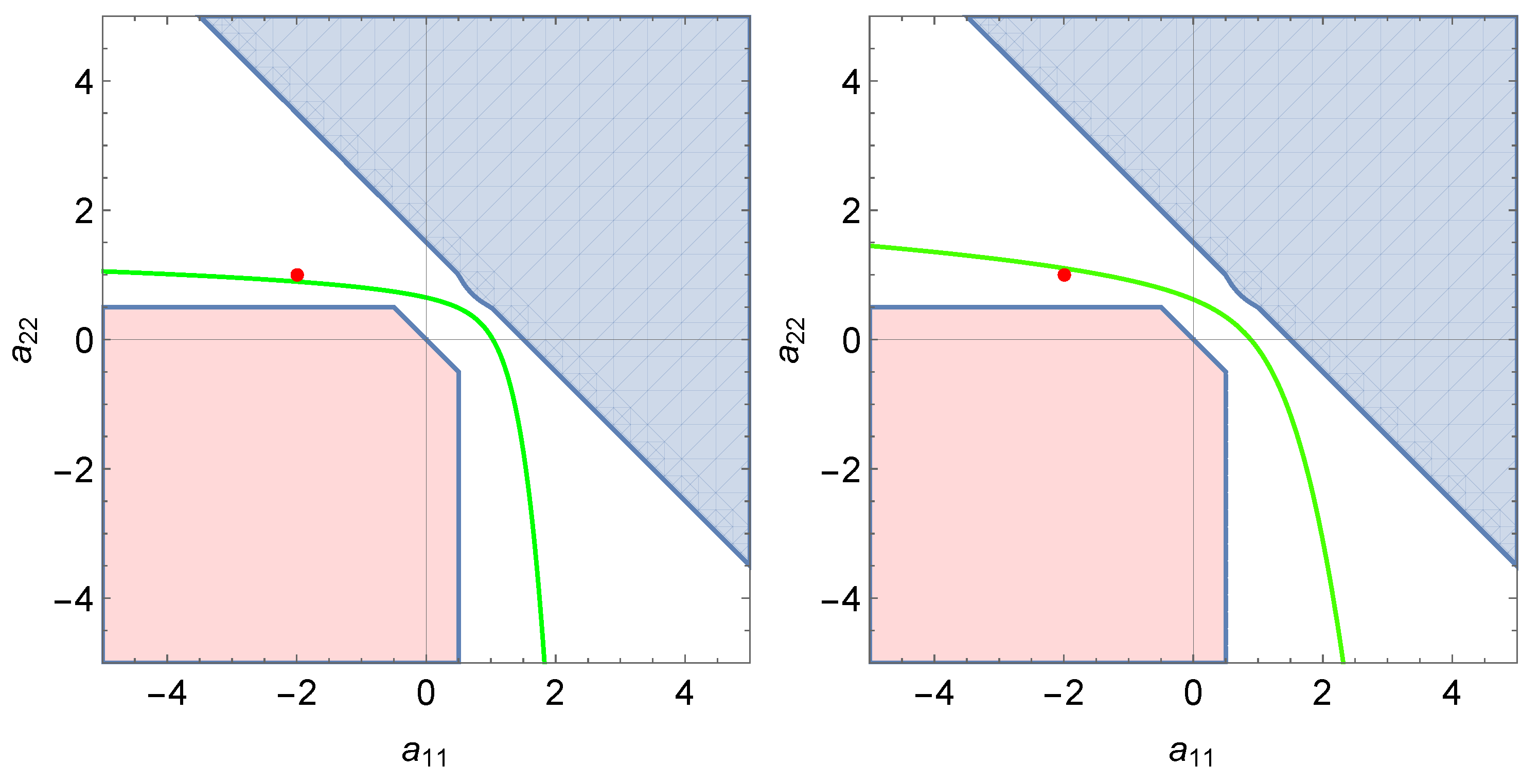
 The curve $\mathrm{\Gamma }(\delta ,q_1,q_2)$ is the graph of a smooth, decreasing, concave bijective function ${\varphi }_{\delta ,q_1,q_2}:\mathbb{R}\to \mathbb{R}$ in the $(a_{11},a_{22})$-plane.

ii. 

 The curve $\mathrm{\Gamma }(\delta ,q_1,q_2)$ lies outside the third quadrant of the $(a_{11},a_{22})$-plane.

Theorem 3

(Fractional-order-dependent stability and instability results).

Let $det\left(A\right)=\delta >0$ and $q_1,q_2\in (0,1]$ arbitrarily fixed. Consider the curve $\mathrm{\Gamma }(\delta ,q_1,q_2)$ and the function ${\varphi }_{\delta ,q_1,q_2}:\mathbb{R}\to \mathbb{R}$ given by Lemma 1.

i. 

 The characteristic Equation (16) has a pair of pure imaginary roots if and only if $(a_{11},a_{22})\in \mathrm{\Gamma }(\delta ,q_1,q_2)$.

ii. 

 System (15) is $\mathcal{O}\left(t^{-q}\right)$-asymptotically stable (with $q=min\{q_1,q_2\}$) if and only if

$$a_{22}<{\varphi }_{\delta ,q_1,q_2}\left(a_{11}\right).$$

iii. 

 If $a_{22}>{\varphi }_{\delta ,q_1,q_2}\left(a_{11}\right)$, system (15) is unstable.

Theorem 3 provides a relatively simple algebraic criterion (in the form of inequalities comprising the elements of the main diagonal of the system’s matrix A as well as its determinant and the fractional orders) that enables us to immediately decide the question of asymptotic stability or instability for a given two-dimensional multi-order system of fractional differential equations. In fact, Theorem 3 may be seen as a generalization of the Routh–Hurwitz stability criterion.

Remark 5.

If $q_1=q_2:=q$, the curve $\mathrm{\Gamma }(\delta ,q_1,q_2)$ reduces to the straight line:

$$a_{11}+a_{22}=2\sqrt{\delta }cos{\displaystyle \frac{q\pi }{2}}.$$

Therefore, Theorem 3 provides that, for equal fractional orders, system (15) is asymptotically stable if and only if

$$Tr\left(A\right)<2\sqrt{det\left(A\right)}cos{\displaystyle \frac{q\pi }{2}}.$$

(17)

The eigenvalues of the system’s matrix A are

$${\lambda }_{1,2}=\frac{Tr\left(A\right)\pm \sqrt{\mathit{Tr}{\left(A\right)}^2-4det\left(A\right)}}{2}$$

and, hence, inequality (17) is equivalent to $|arg{\lambda }_{1,2}|>\frac{q\pi }{2}$. Consequently, for two-dimensional systems, the conclusion of Matignon’s theorem is recovered as a particular case of Theorem 3.

Remark 6.

The asymptotic stability of the two-dimensional integer order system $\dot{y}=Ay$ does not directly imply the asymptotic stability of system (15) for any fractional orders $(q_1,q_2)\in {(0,1]}^2$. We can only state, based on Remark 4, that, if the integer order system $\dot{y}=Ay$ is asymptotically stable, then so is system (15) with equal fractional orders $q_1=q_2$.

Example 2.

Let us consider the system

$$\left\{\begin{array}{c}{}^{\mathrm{C}}{D}^{q_1}{y}_1\left(t\right)=a_{11}{y}_1\left(t\right)+a_{12}{y}_2\left(t\right)\hfill \\ {}^{\mathrm{C}}{D}^{q_2}{y}_2\left(t\right)=a_{21}{y}_1\left(t\right)+a_{22}{y}_2\left(t\right)\hfill \end{array}\right.\mathrm{with}A=\left(a_{ij}\right)=\left(\begin{array}{cc}-2& 0.5\\ -5& 1\end{array}\right)$$

(18)

where $q_1,q_2\in (0,1]$. As $Tr\left(A\right)=-1<0$ and $det\left(A\right)=0.5>0$, the Routh–Hurwith stability test guarantees that, for $q_1=q_2=1$, system (18) is asymptotically stable (see left plot in Figure 5); the eigenvalues of the matrix A are ${\lambda }_{1,2}=-\frac{1}{2}(1\pm i)$. Therefore, for equal fractional orders $q_1=q_2\in (0,1)$, system (18) is also asymptotically stable (see left plot in Figure 5); this can also be verified by inequality (17).

However, for $q_1=0.2$ and $q_2=1$, system (18) is unstable (see right plot in Figure 5). Indeed, applying Theorem 3, system (18) with $(q_1,q_2)=(0.2,1)$ is unstable if

$$a_{22}>{\varphi }_{\delta ,q_1,q_2}\left(a_{11}\right),$$

where $a_{11}=-2$, $a_{22}=1$, $\delta =det\left(A\right)=0.5$ and, based on the notations from Lemma 1:

$${\varphi }_{\delta ,q_1,q_2}\left(a_{11}\right)={\delta }^{\frac{q_2}{q_1+q_2}}h(-{\omega }^{*},q_1,q_2)$$

where ${\omega }^{*}$ is the unique root of the equation

$$a_{11}={\delta }^{\frac{q_1}{q_1+q_2}}h({\omega }^{*},q_1,q_2).$$

Numerically solving this algebraic equation, we compute ${\omega }^{*}=-2.19664$ and, therefore, we also obtain ${\varphi }_{\delta ,q_1,q_2}\left(a_{11}\right)=0.895383$. As $a_{22}=1$, it follows that the instability condition $a_{22}>{\varphi }_{\delta ,q_1,q_2}\left(a_{11}\right)$ is satisfied (see left plot of Figure 6).

Furthermore, it is important to emphasize that Theorem 3 can also be applied when at least one of the fractional orders is irrational. For example, choosing $q_1=\frac{1}{\pi }$ and $q_2=1$, in a similar way as before, we compute ${\varphi }_{\delta ,q_1,q_2}\left(a_{11}\right)=1.10307$, and hence $a_{22}<{\varphi }_{\delta ,q_1,q_2}\left(a_{11}\right)$, which means that system (18) with $q_1=\frac{1}{\pi }$ and $q_2=1$ is asymptotically stable (see right plot of Figure 6).

Figure 7 showes region of fractional orders $(q_1,q_2)$ for which system (18) is globally asymptotically stable.

The next step is to seek necessary and sufficient conditions which ensure the asymptotic stability or instability of system (15) for any choice of the fractional orders. A complete investigation of the family of curves $\mathrm{\Gamma }(\delta ,q_1,q_2)$ leads to the following fractional-order independent stability and instability results [17]:

Theorem 4

(Fractional-order independent instability results).

i. 

 If $det\left(A\right)<0$, system (15) is unstable, regardless of the fractional orders $q_1$ and $q_2$.

ii. 

 If $det\left(A\right)>0$, system (15) is unstable regardless of the fractional orders $q_1$ and $q_2$ if and only if one of the following conditions holds:

$$\left\{\begin{array}{cc}& a_{11}+a_{22}\ge det\left(A\right)+1or\hfill \\ & a_{11}>0,a_{22}>0,a_{11}{a}_{22}\ge det\left(A\right).\hfill \end{array}\right.$$

Theorem 5

(Fractional-order-independent stability results). System (15) is asymptotically stable, regardless of the fractional orders $q_1,q_2\in (0,1]$ if and only if the following inequalities are satisfied:

$$a_{11}+a_{22}<0<det\left(A\right)andmax\{a_{11},a_{22}\}<min\{1,det\left(A\right)\}.$$

The previous theorems provide easily verifiable necessary and sufficient conditions which ensure the asymptotic stability or instability of the two-dimensional system (15), for any choice of the fractional orders $q_1,q_2\in (0,1]$. These conditions are expressed as simple inequalities involving the main diagonal elements $a_{11}$ and $a_{22}$ as well as the determinant $det\left(A\right)$ of the system’s matrix. On one hand, if $det\left(A\right)<0$, Theorem 4 provides that system (15) is unstable, for any choice of the fractional orders $q_1,q_2\in (0,1]$. Hence, we will focus our attention on the case $\delta =det\left(A\right)>0$. Let us denote by $R_s$ and by $R_u$ the fractional-order independent stability and instability regions given by Theorems 4 and 5:

$$\begin{array}{cc}\hfill R_u& =\{(a_{11},a_{22},\delta )\in {\mathbb{R}}^2\times (0,\infty ):a_{11}+a_{22}\ge \delta +1\mathrm{or}{a}_{11}>0,a_{22}>0,a_{11}{a}_{22}\ge \delta \}\hfill \\ \hfill R_s& =\{(a_{11},a_{22},\delta )\in {\mathbb{R}}^2\times (0,\infty ):a_{11}+a_{22}<0\mathrm{and}max\{a_{11},a_{22}\}<min\{1,\delta \}\}\hfill \end{array}$$

The regions $R_u$ and $R_s$ are plotted in Figure 8. The intersections of these regions with the $\delta =det\left(A\right)=6$ plane are shown in Figure 9. Moreover, it can be verified [17] that the union of all the curves $\mathrm{\Gamma }(\delta ,q_1,q_2)$ (for $\delta >0$ and $q_1,q_2\in (0,1]$) represents the complementary of $R_s\cup R_u$ (see Figure 9).

Remark 7.

The classical Routh–Hurwitz stability test for two-dimensional systems of the form $\dot{y}=Ay$ provide that the system is asymptotically stable if and only if $\mathit{Tr}\left(\mathrm{A}\right)<0$ and $det\left(A\right)>0$. However, based on Theorem 5, the additional inequality $max\{a_{11},a_{22}\}<min\{1,det\left(A\right)\}$ has to be verified in order to ensure the asymptotic stability of the fractional-order system (15), regardless of the choice of fractional orders $q_1$ and $q_2$.

Example 3.

It is easy to see that, if system (18) is considered, as $a_{11}=-2$, $a_{22}=1$ and $det\left(A\right)=0.5$, even though the Routh–Hurwitz conditions $\mathit{Tr}\left(A\right)<0$ and $det\left(A\right)>0$ are fulfilled, the additional additional inequality $max\{a_{11},a_{22}\}<min\{1,det\left(A\right)\}$ does not hold, and hence system (18) is not asymptotically stable for any choice of the fractional orders $q_1,q_2\in (0,1]$. Indeed, as we have seen in Example 2, for $q_1=0.2$ and $q_2=1$, system (18) is unstable.

In conclusion, based on the previously described results, the following steps should be undertaken for the stability analysis of a two-dimensional system of FDEs:

1.

 if $det\left(A\right)<0$, then the system is unstable, for any choice of the fractional orders $q_1,q_2\in (0,1]$, based on Theorem 4;

2.

 if $(a_{11},a_{22},det\left(A\right))\in R_u$, then the system is unstable, for any choice of the fractional orders $q_1,q_2\in (0,1]$, based on Theorem 4;

3.

 if $(a_{11},a_{22},det\left(A\right))\in R_s$, then the system is asymptotically stable, for any choice of the fractional orders $q_1,q_2\in (0,1]$, based on Theorem 5;

4.

 if $(a_{11},a_{22},det\left(A\right))\notin R_s\cup R_u$, then the stability properties of the system depend on choice of the fractional orders $q_1,q_2\in (0,1]$ and Theorem 3 should be applied.

The results described in this section, particularly Theorems 3–5, give a comprehensive method to assess stability properties of two-dimensional fractional-order systems. However, the generalization of these results to higher dimensional fractional-order systems still remains an open question.

5.2. Stability of Higher Dimensional Systems of FDEs with Specific Structures

Consider that the matrix A of the linear system (12) has a block-triangular structure:

$$A=\left(\begin{array}{cccc}{A}_{11}& A_{12}& \dots & A_{1p}\\ & A_{22}& \dots & A_{2p}\\ & & \ddots & ⋮\\ & & & A_{pp}\end{array}\right)$$

where $A_{ii}\in {\mathbb{R}}^{d_i\times d_i}$, for $i=\overline{1,m}$ and $A_{ii}\in {\mathbb{R}}^{2\times 2}$ for $i=\overline{m+1,p}$, such that

$$\sum _{i=1}^m{d}_i+2(p-m)=n.$$

We also assume that

$$q=(\underset{d_1\mathrm{times}}{\underbrace{q_1,q_1,\dots ,q_1}},\dots ,\underset{d_m\mathrm{times}}{\underbrace{q_m,q_m,\dots ,q_m}},q_{m+1}^1,q_{m+1}^2,\dots q_p^1,q_p^2)\in {(0,1]}^n.$$

In this case, the characteristic equation associated with system (12) is

$$\prod _{i=1}^{m}det(s^{q_i}I-A_{ii})·\prod _{i=m+1}^{p}det(\mathrm{diag}(s^{q_i^2},s^{q_i^2})-A_{ii})=0$$

(19)

Therefore, combining Matignon’s theorem (Theorem 1) and Theorem 3, the following statements are obtained:

• system (12) is asymptotically stable if and only if

  -

  $\sigma \left(A_{ii}\right)\subset S_{q_i}=\left\{\lambda \in \mathbb{C}:|arg\left(\lambda \right)|>\frac{q_i\pi }{2}\right\}$ for any $i=\overline{1,m}$ and

  -

  $A_{ii}^{22}<{\varphi }_{{\delta }_i,q_i^1,q_i^2}\left(A_{ii}^{11}\right)$, for any $i=\overline{m+1,p}$, where $A_{ii}^{11}$ and $A_{ii}^{22}$ are the main diagonal elements of matrix $A_{ii}$, ${\delta }_i=det\left(A_{ii}\right)$ and $\varphi$ is defined in Lemma 1.

• system (12) is unstable if at least one of the following holds:

  -

  there exists $i\in \{1,2,\dots m\}$ such that the matrix $A_{ii}$ has at least one eigenvalue $\lambda$ such that $|arg\left(\lambda \right)|<\frac{q_i\pi }{2}$ or

  -

  there exists $i\in \{m+1,\dots ,p\}$ such that $A_{ii}^{22}>{\varphi }_{{\delta }_i,q_i^1,q_i^2}\left(A_{ii}^{11}\right)$, where $A_{ii}^{11}$ and $A_{ii}^{22}$ are the main diagonal elements of matrix $A_{ii}$, ${\delta }_i=det\left(A_{ii}\right)$ and $\varphi$ is defined in Lemma 1.

5.3. Stability of Higher Dimensional Systems of FDEs with Special Fractional Orders

Let us consider the following n-dimensional linear multi-order system of fractional differential equations:

$${}^{\mathrm{C}}{D}^{q_i}{y}_i\left(t\right)=\sum _{j=1}^n{a}_{ij}{y}_j\left(t\right),i=\overline{1,n},$$

(20)

where $q_i\in (0,1]$, $a_{ij}\in \mathbb{R}$ and $n\ge 3$.

If the coefficient matrix of the system is not of a triangular or block triangular form as considered in the previous section, one can not provide a comprehensive stability theory. Still, an approach that works under certain restrictions on the fractional orders of the Caputo derivatives has been developed in [14]. We will next recall the general results obtained by the mentioned authors.

Suppose $q_j\in (0,1]$, for any $j=\overline{1,n}$ and that there exists $q^{*}\in (0,1]$ and ${\rho }_j\in \mathbb{Q}$ such that $q_j={\rho }_j{q}^{*}.$ It follows that there exists $r_j,s_j\in \mathbb{N}$ for $j=\overline{1,n}$ such that $\gcd (r_j,s_j)=1$ and ${\rho }_j={\displaystyle \frac{r_j}{s_j}}$. Let s be the least common multiple of the denominators $s_j$. Then, for any j, there exists ${\alpha }_j\in \mathbb{N}$ such that

$$q_j={\displaystyle \frac{q^{*}{\alpha }_j}{s}}\left({\alpha }_j={\displaystyle \frac{s{r}_j}{s_j}}\right).$$

We can rewrite the $j$-th equation of system (20) as an equivalent system of ${\alpha }_j$ differential equations having the order ${\displaystyle \frac{q^{*}}{s}}$. It follows that system (20) can be expressed as a system of $n^{*}={\displaystyle \sum _{j=1}^n}{\alpha }_j$ equations of order ${\displaystyle \frac{q^{*}}{s}}$:

$${}^{\mathrm{C}}{D}^{q^{*}/s}{y}^{*}\left(t\right)=A^{*}{y}^{*}\left(t\right),$$

(21)

where $A^{*}$ has the following block structure

$$A^{*}=\left(\begin{array}{cccc}{A}_{11}& A_{12}& \cdots & A_{1n}\\ A_{21}& A_{22}& \cdots & A_{2n}\\ ⋮& ⋮& \ddots & ⋮\\ A_{n1}& A_{n2}& \cdots & A_{nn}\end{array}\right)$$

with $A_{jk}\in {\mathbb{R}}^{{\alpha }_j\times {\alpha }_k}$,

$$A_{jj}=\left(\begin{array}{cccccc}0& 1& 0& \cdots & 0& 0\\ 0& 0& 1& \cdots & 0& 0\\ ⋮& ⋮& ⋮& \ddots & 0& 0\\ 0& 0& 0& \cdots & 0& 1\\ a_{jj}& 0& 0& \cdots & 0& 0\end{array}\right),j=\overline{1,n}$$

and

$$A_{jk}=\left(\begin{array}{cccc}0& 0& \cdots & 0\\ ⋮& ⋮& \ddots & 0\\ 0& 0& \cdots & 0\\ a_{jk}& 0& \cdots & 0\end{array}\right),j,k=\overline{1,n},j\ne k.$$

Even though the dimension $n^{*}$ of the system may be significantly higher than the dimension n of the original system (20), resulting in higher computational costs, all the equations of the new system (21) now have the same fractional order, giving an advantage in studying the stability properties of the solutions of the system.

We expose the main result of this section, based on [14], which gives us stability criteria involving the components of the matrix $A^{*}$.

Theorem 6.

Suppose that $q_j\in (0,1]$ for any j and there exists $q^{*}\in (0,1]$ and ${\rho }_j\in \mathbb{Q}$ such that $q_j={\rho }_j{q}^{*}$, for all j. Then, all the solutions of system (20) converge to zero at infinity if the eigenvalues ${\lambda }_j^{*}$ of the associated system’s coefficient matrix $A^{*}$ satisfy

$$|arg{\lambda }_j^{*}|>{\displaystyle \frac{\pi q^{*}}{2s}},\forall j=\overline{1,n},$$

with s being the least common multiple of the denominators of ${\rho }_j$.

Example 4.

Again, we reconsider system (18) with $q_1=0.2$ and $q_2=1$. In this case, the matrix $A^{*}$ given by the above procedure is

$$A^{*}=\left(\begin{array}{cccccc}{a}_{11}& a_{12}& 0& 0& 0& 0\\ 0& 0& 1& 0& 0& 0\\ 0& 0& 0& 1& 0& 0\\ 0& 0& 0& 0& 1& 0\\ 0& 0& 0& 0& 0& 1\\ a_{21}& a_{22}& 0& 0& 0& 0\end{array}\right)=\left(\begin{array}{cccccc}-2& 0.5& 0& 0& 0& 0\\ 0& 0& 1& 0& 0& 0\\ 0& 0& 0& 1& 0& 0\\ 0& 0& 0& 0& 1& 0\\ 0& 0& 0& 0& 0& 1\\ -5& 1& 0& 0& 0& 0\end{array}\right)$$

and the system (18) is equivalent to a system of six fractional-order differential equations with the same order $q=q_1=0.2$. The matrix $A^{*}$ has a pair of complex conjugated eigenvalues $(\lambda ,\overline{\lambda })$, $\lambda =0.543842+i0.133131$ such that $|arg\left(\lambda \right)|=0.240076<0.1\pi =\frac{q\pi }{2}$. Hence, based on Matignon’s theorem, system (18) is unstable for $q_1=0.2$ and $q_2=1$. Therefore, this is in good agreement with the results obtained in Example 2, based on Theorem 3.

However, it is important to note that cases $q_1=\frac{1}{\pi }$ and $q_2=1$ cannot be investigated using the technique provided by Theorem 6.

6. Conclusions

An extensive analysis of stability properties of linear systems of FDEs has been provided. This analysis is of importance to describe the asymptotic behavior of physical systems when modeled by means of FDEs. Both single-order and multi-order systems have been studied, reviewing the most important theoretical results that have been obtained so far in the literature. The role of the Mittag–Leffler function, and of its derivatives, has been highlighted and a presentation of their asymptotic behavior has been proposed. We have seen that, unlike systems of integer order, coefficients of the systems are not sufficient to describe stability properties of solutions, due to the tight dependence on the order of the fractional derivatives. This dependence becomes more and more difficult to investigate in systems incorporating derivatives of different order, as we have observed from the analysis of two-dimensional systems. Stability analysis of multi-order higher dimensional systems is still an open problem which deserves to be investigated with more attention; with this work, a first contribution has been provided by examining systems with some specific structures, and we hope these results will stimulate the analysis of more general systems.

References

- Li, C.; Zhang, F. A survey on the stability of fractional differential equations. Eur. Phys. J. Spec. Top. 2011, 193, 27–47. [Google Scholar] [CrossRef]
- Rivero, M.; Rogosin, S.V.; Tenreiro Machado, J.A.; Trujillo, J.J. Stability of fractional order systems. Math. Probl. Eng. 2013, 2013, 356215. [Google Scholar] [CrossRef]
- Li, C.; Ma, Y. Fractional dynamical system and its linearization theorem. Nonlinear Dyn. 2013, 71, 621–633. [Google Scholar] [CrossRef]
- Wang, Z.; Yang, D.; Zhang, H. Stability analysis on a class of nonlinear fractional-order systems. Nonlinear Dyn. 2016, 86, 1023–1033. [Google Scholar] [CrossRef]
- Tuan, H.T.; Trinh, H. Global attractivity and asymptotic stability of mixed-order fractional systems. IET Control Theory Appl. 2020, 14, 1240–1245. [Google Scholar] [CrossRef]
- Matignon, D. Stability results for fractional differential equations with applications to control processing. Comput. Eng. Syst. Appl. 1996, 2, 963–968. [Google Scholar]
- Sabatier, J.; Farges, C. On stability of commensurate fractional order systems. Int. J. Bifurc. Chaos 2012, 22, 1250084. [Google Scholar] [CrossRef]
- Deng, W.; Li, C.; Lu, J. Stability analysis of linear fractional differential system with multiple time delays. Nonlinear Dyn. 2007, 48, 409–416. [Google Scholar] [CrossRef]
- Deng, W.; Li, C.; Guo, Q. Analysis of fractional differential equations with multi-orders. Fractals 2007, 15, 173–182. [Google Scholar] [CrossRef]
- Petras, I. Stability of fractional-order systems with rational orders. Fract. Calc. Appl. Anal. 2009, 12, 269–298. [Google Scholar]
- Diethelm, K. Multi-term fractional differential equations, multi-order fractional differential systems and their numerical solution. J. Eur. Syst. Autom. 2008, 42, 665–676. [Google Scholar] [CrossRef]
- Bonnet, C.; Partington, J.R. Coprime factorizations and stability of fractional differential systems. Syst. Control Lett. 2000, 41, 167–174. [Google Scholar] [CrossRef]
- Trächtler, A. On BIBO stability of systems with irrational transfer function. arXiv 2016, arXiv:1603.01059. [Google Scholar]
- Diethelm, K.; Siegmund, S.; Tuan, H. Asymptotic behavior of solutions of linear multi-order fractional differential systems. Fract. Calc. Appl. Anal. 2017, 20, 1165–1195. [Google Scholar] [CrossRef] [Green Version]
- Brandibur, O.; Kaslik, E. Stability properties of a two-dimensional system involving one Caputo derivative and applications to the investigation of a fractional-order Morris-Lecar neuronal model. Nonlinear Dyn. 2017, 90, 2371–2386. [Google Scholar] [CrossRef] [Green Version]
- Brandibur, O.; Kaslik, E. Stability of two-component incommensurate fractional-order systems and applications to the investigation of a FitzHugh-Nagumo neuronal model. Math. Methods Appl. Sci. 2018, 41, 7182–7194. [Google Scholar] [CrossRef] [Green Version]
- Brandibur, O.; Kaslik, E. Exact stability and instability regions for two-dimensional linear autonomous multi-order systems of fractional-order differential equations. Fract. Calc. Appl. Anal. 2021, 24, 225–253. [Google Scholar] [CrossRef]
- Atanackovic, T.; Dolicanin, D.; Pilipovic, S.; Stankovic, B. Cauchy problems for some classes of linear fractional differential equations. Fract. Calc. Appl. Anal. 2014, 17, 1039–1059. [Google Scholar] [CrossRef] [Green Version]
- Jiao, Z.; Chen, Y.Q. Stability of fractional-order linear time-invariant systems with multiple noncommensurate orders. Comput. Math. Appl. 2012, 64, 3053–3058. [Google Scholar] [CrossRef] [Green Version]
- Čermák, J.; Kisela, T. Asymptotic stability of dynamic equations with two fractional terms: Continuous versus discrete case. Fract. Calc. Appl. Anal. 2015, 18, 437. [Google Scholar] [CrossRef]
- Čermák, J.; Kisela, T. Stability properties of two-term fractional differential equations. Nonlinear Dyn. 2015, 80, 1673–1684. [Google Scholar] [CrossRef]
- Brandibur, O.; Kaslik, E. Stability analysis of multi-term fractional-differential equations with three fractional derivatives. J. Math. Anal. Appl. 2021, 495, 124751. [Google Scholar] [CrossRef]
- Haubold, H.; Mathai, A.; Saxena, R. Mittag–Leffler Functions and Their Applications. J. Appl. Math. 2011, 2011, 298628. [Google Scholar] [CrossRef] [Green Version]
- Prabhakar, T.R. A singular integral equation with a generalized Mittag–Leffler function in the kernel. Yokohama Math. J. 1971, 19, 7–15. [Google Scholar]
- Paris, R.B. Exponentially small expansions in the asymptotics of the Wright function. J. Comput. Appl. Math. 2010, 234, 488–504. [Google Scholar] [CrossRef] [Green Version]
- Paris, R.B. Asymptotics of the Special Functions of Fractional Calculus. In Handbook of Fractional Calculus with Applications; De Gruyter: Berlin, Germany, 2019; Volume 1, pp. 297–325. [Google Scholar]
- Giusti, A.; Colombaro, I.; Garra, R.; Garrappa, R.; Polito, F.; Popolizio, M.; Mainardi, F. A practical guide to Prabhakar fractional calculus. Fract. Calc. Appl. Anal. 2020, 23, 9–54. [Google Scholar] [CrossRef] [Green Version]
- Garra, R.; Garrappa, R. The Prabhakar or three parameter Mittag-Leffler function: Theory and application. Commun. Nonlinear Sci. Numer. Simul. 2018, 56, 314–329. [Google Scholar] [CrossRef] [Green Version]
- Giusti, A. General fractional calculus and Prabhakar’s theory. Commun. Nonlinear Sci. Numer. Simul. 2020, 83, 105114. [Google Scholar] [CrossRef] [Green Version]
- Kochubei, A.N. General fractional calculus, evolution equations, and renewal processes. Integral Equ. Oper. Theory 2011, 71, 583–600. [Google Scholar] [CrossRef] [Green Version]
- Brunner, H. Volterra Integral Equations: An Introduction to Theory and Applications; Cambridge University Press: Cambridge, UK, 2017; Volume 30. [Google Scholar]
- Gripenberg, G.; Londen, S.O.; Staffans, O. Volterra Integral and fUnctional Equations; Cambridge University Press: Cambridge, UK, 1990; Volume 34. [Google Scholar]
- Lubich, C. A stability analysis of convolution quadratures for Abel-Volterra integral equations. IMA J. Numer. Anal. 1986, 6, 87–101. [Google Scholar] [CrossRef]
- Tsalyuk, Z. Volterra integral equations. J. Sov. Math. 1979, 12, 715–758. [Google Scholar] [CrossRef]
- Doetsch, G. Introduction to the Theory and Application of the Laplace Transformation; Springer: Berlin/Heidelberg, Germany, 1974. [Google Scholar]
- Horn, R.A.; Johnson, C.R. Matrix Analysis, 2nd ed.; Cambridge University Press: Cambridge, UK, 2013; p. xviii+643. [Google Scholar]
- Garrappa, R.; Popolizio, M. Computing the matrix Mittag-Leffler function with applications to fractional calculus. J. Sci. Comput. 2018, 77, 129–153. [Google Scholar] [CrossRef] [Green Version]
Publisher’s Note: MDPI stays neutral with regard to jurisdictional claims in published maps and institutional affiliations. |
© 2021 by the authors. Licensee MDPI, Basel, Switzerland. This article is an open access article distributed under the terms and conditions of the Creative Commons Attribution (CC BY) license (https://creativecommons.org/licenses/by/4.0/).
Share and Cite
Brandibur, O.; Garrappa, R.; Kaslik, E. Stability of Systems of Fractional-Order Differential Equations with Caputo Derivatives. Mathematics 2021, 9, 914. https://doi.org/10.3390/math9080914
Brandibur O, Garrappa R, Kaslik E. Stability of Systems of Fractional-Order Differential Equations with Caputo Derivatives. Mathematics. 2021; 9(8):914. https://doi.org/10.3390/math9080914
Chicago/Turabian StyleBrandibur, Oana, Roberto Garrappa, and Eva Kaslik. 2021. "Stability of Systems of Fractional-Order Differential Equations with Caputo Derivatives" Mathematics 9, no. 8: 914. https://doi.org/10.3390/math9080914