Abstract
Incineration leachate is a hazardous liquid waste that requires careful management due to its high levels of organic and inorganic pollutants, and it can have serious environmental and health implications if not properly treated and monitored. This study applied a novel electronic nose to monitor the microbial communities and chemical characteristics of incineration leachate. The e-nose data were aggregated using principal component analysis (PCA) and T-distributed stochastic neighbor embedding (TSNE). Random forest (RF) and gradient-boosted decision tree (GBDT) algorithms were employed to establish relationships between the e-nose signals and the chemical characteristics (such as pH, chemical oxygen demand, and ammonia nitrogen) and microbial communities (including Proteobacteria, Firmicutes, and Bacteroidetes) of the incineration leachate. The PCA-GBDT models performed well in recognizing leachate samples, achieving 100% accuracy for the training set and 98.92% accuracy for the testing data without overfitting. The GBDT models based on the original data performed exceptionally well in predicting changes in chemical parameters, with R2 values exceeding 0.99 for the training set and 0.86 for the testing set. The PCA-GBDT models also demonstrated superior performance in predicting microbial community composition, achieving R2 values above 0.99 and MSE values below 0.0003 for the training set and R2 values exceeding 0.86 and MSE values below 0.015 for the testing set. This research provides an efficient monitoring method for the effective enforcement and implementation of monitoring programs by utilizing e-noses combined with data mining to provide more valuable insights compared with traditional instrumental measurements.
1. Introduction
Incineration leachate is a complex type of organic wastewater that is generated during the treatment of municipal solid waste that includes proteins, volatile fatty acids, and refractory organics [1]. The treatment of incineration leachate can pose a challenge because of its intricate structure and potentially harmful contents, such as carcinogens and toxins. Proper monitoring and treatment are crucial in order to prevent these pollutants from polluting the surrounding environment [2,3].
The primary emphasis of research on incineration leachate has been on investigating the properties of the concentrated leachate [4], the molecular changes that occur in organic matter during treatment [5,6], and the alterations in microorganisms [7,8] that occur during different processes. These studies indicate that the headspace gas above leachate may contain valuable information for monitoring or processing the leachate. So far, only a small number of comprehensive studies have been carried out to extract information from large quantities of raw data on the types, concentrations, and changes in these materials.
An electronic nose (e-nose) is a promising candidate designed to mimic the sense of the human nose by detecting and analyzing volatile organic compounds (VOCs) in headspace gas [9]. With a combination of sensors, such as metal oxide sensors, conducting polymers, and quartz crystal microbalance sensors, an e-nose can measure the changes in electrical resistance or impedance that result from the interaction of headspace gas in samples [10]. Sensor data are then processed and analyzed using machine learning to identify specific compounds and determine their concentration [11]. With the advantage of providing rapid and non-invasive analyses, e-noses are suitable for use in a wide range of industries and applications [12,13]. However, studies on leachate detection based on e-nose technology are rare, according to our best knowledge.
For incineration leachate, the variety and quantity of microorganisms in each process are quite important, as they result in different treatment effects of waste incineration plants [14]. The relationship between headspace gas and microorganisms in leachate is noteworthy and complicated [15]. Microorganisms consume oxygen and carbon dioxide in headspace gas through respiration and metabolism, and they produce nitrogen, nitrous oxide, and other organic substances [16]. Therefore, microorganisms play important regulatory roles in the composition of headspace gas. In addition, the growth of microorganisms is influenced by the oxygen content and pH value of the leachate [17], which consequently have feedback effects on the headspace gas and leachate. Overall, the relationship between headspace gas and microorganisms is a complex system of mutual influence and regulation [18]. Studying this relationship is essential for understanding the biological processes of leachate and optimizing leachate treatment technology. However, molecular biology techniques have low specificity and require a significant amount of time to perform. In this study, e-nose technology was applied to mine headspace gas information to study microorganism changes.
Our main objectives were: (1) to monitor the changes in leachate headspace gas based on e-nose technology; (2) to process sensor signals based on data reduction and machine learning (random forest and gradient-boosted decision tree); and (3) to mine information on the relationship between headspace gas and microorganisms in leachate based on e-nose data. This research offers a more efficient monitoring method for the effective enforcement and implementation of monitoring programs by utilizing e-nose technology combined with machine learning to analyze the relationships among leachate gas emissions, chemical parameters, and microorganisms, thus providing more valuable insights compared with traditional instrumental measurements.
2. Material and Methods
2.1. Sample Collection
Leachate incineration samples were obtained from a local waste incineration power plant (Xiaoshan Jinjiang Green Energy Co., Ltd., Hangzhou, China), as a subsidiary of Zheneng Jinjiang Environment Holding Co., Ltd., (Hangzhou, China). This company is a pioneer and leader in China’s WTE (waste-to-energy) industry. The incineration power plant is located in the southeast part of Hangzhou next to the East China Sea and has a treatment scale of 1900 tons per day of WTE.
On 15 August 2022, six water outlets provided leachate samples. As shown in Figure 1, the samples were labeled as LRW (leachate raw water), LE (leachate effluent), internal circulation reactor effluent (ICRE), AeroE (aerobic effluent), ANE (anaerobic effluent), and MBRE (MBR effluent). The samples were stored in a fridge at below 4 °C and transported to a lab for analysis.
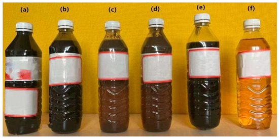
Figure 1.
Leachate samples from six collections: (a) leachate raw water (LRW); (b) leachate effluent (LE); (c) internal circulation reactor effluent (ICRE); (d) aerobic effluent (AeroE); (e) anaerobic effluent (ANE); (f) MBR effluent (MBRE).
2.2. E-Nose Diagnose for Leachate Characteristic in the Headspace Gas
The headspace gas of the leachate samples was detected with a commercial PEN2 E-Nose (Airsense Analytics, GmBH, Schwerin, Germany). This device’s core components are MOS sensors, as described in Table 1. The MOS sensors transform the gas types and concentrations into electrochemical signals (R/R0, where R is the sensor resistance in the sample headspace gas and R0 is the sensor resistance in clear air), presenting complementary information of the whole headspace gas instead of specific materials.

Table 1.
Sensors and their main applications in the commercial PEN2 E-Nose [19].
To protect the e-nose sensors, Wahaha purified water with a conductivity of ≤5 μs/cm (Hangzhou Wahaha Group Co., Ltd., Hangzhou, China) was adopted to dilute the leachate samples. The ratio of purified water and leachate was 4:1. First, 5 mL of liquid diluted leachate samples was placed into a 500 mL beaker sealed by plastic wrap, and the beaker was kept still for 30 min. The gas flow rate was set to 200 mL/min, and 80 s were taken for e-nose detection. After detection, the sensor chamber was cleaned with clean air. Then, 144 samples (24 samples for each water outlet, with six water outlets) were selected.
2.3. Chemical Parameters Detection for Incinerator Leachate
Chemical parameters (pH, chemical oxygen demand (COD), and ammonia (NH4+-N)) were detected on site according to the national standard. The electrode method [20] was applied to detect pH values. The chlorine emendation method [21] was used to detect the contents of COD instead of the dichromate method. The concentration of ammonia nitrogen was measured using Nessler’s reagent spectrophotometry [22].
2.4. Microbial Community and Functional Potential
Genomic DNA was isolated from the sediment of the leachate deposit and quantified using a NanoDrop 2000 Spectrophotometer (Thermo Fisher Technology, Waltham, MA, USA). The quality of the DNA was further confirmed with gel electrophoresis. Six samples (LRW, LE, ICRE, AeroE, ANE, and MBRE) were analyzed. To amplify the target genomic 16S rRNA (V3–V4 region), we utilized the PCR primer sets 338F (5′-ACTCCTACGG-GAGGCAGCA-3′) and 806R (5′-TCGGACTACHVGGGTWTCTAAT-3′) in conjunction with an Applied Biosystems 2720 thermal cycler. To amplify the target genomic 16S rRNA (V3–V4 region), we employed an Applied Biosystems 2720 thermal cycler and the PCR primer sets 338F (5′-ACTCCTACGG-GAGGCAGCA-3′) and 806R (5′-TCGGACTACHVGGGTWTCTAAT-3′). The amplification program consisted of an initial denaturation step at 98 °C for 2 min, followed by 30 cycles of denaturation at 98 °C for 15 s, annealing at 55 °C for 30 s, and extension at 72 °C for 30 s. A final extension step was performed at 72 °C for 5 min. After amplification, the products were purified using the Axygen gel recovery kit and quantified with a microplate reader (BioTek, FLx800). The sequencing results were clustered into OTUs at a 97% similarity level using the QIIME software. Comparisons of bacterial richness and diversity were performed using the Chao1, ACE, Shannon–Wiener, and Simpson indices. Analyses were performed using the Personalbio online analysis platform.
2.5. Data Reduction for E-Nose Sensor Signals
2.5.1. Principal Component Analysis
Principal component analysis (PCA) is a mathematical technique utilized to decrease the dimensionality of a dataset by mapping the data onto a space with fewer dimensions. PCA works by finding the directions in data that have the highest variance (i.e., the directions that contain the most information) and projecting the data onto these directions. This results in a new set of variables, called principal components (PCs), that are orthogonal to each other and capture the most important information in the data. This method can be used to visualize high-dimensional data in lower dimensions. Below is an overview of the details of PCA:
- (1).
- Normalize the continuous input data range.
- (2).
- Calculate the covariance matrix to detect associations.
- (3).
- Perform eigenvalue and eigenvector computations on the covariance matrix to discover the dominant factors.
- (4).
- Generate a feature vector to determine which principal components should be retained.
- (5).
- Transform the data onto the principal component axes.
2.5.2. T-Distributed Stochastic Neighbor Embedding
T-distributed stochastic neighbor embedding (TSNE) is also a dimensionality reduction technique that is often used to visualize high-dimensional data in lower dimensions by preserving the distances between data points. TSNE allows data to be visualized on a two- or three-dimensional scatter plot where similar data points are clustered together and dissimilar data points are separated from each other. It is effective at visualizing data with complex, non-linear structures, such as clusters of different shapes and sizes. The details of TSNE are as follows:
- (1).
- Find the pairwise similarity between nearby points in a high-dimensional space.
- (2).
- Map the points in high-dimensional space to a low-dimensional map according to their pairwise similarity.
- (3).
- Use gradient descent based on Kullback–Leibler divergence to minimize the difference between two points and find a low-dimensional representation of the data.
- (4).
- Calculate the similarity between two points in low-dimensional space using a Student distribution.
2.6. Data Treatment
2.6.1. Random Forest
A random forest (RF) is an ensemble learning algorithm used for classification and regression tasks. An ensemble is a collection of individual models that are combined to make a single, more powerful model. An RF consists of individual decision trees that are trained on different subsets of data and then combined to perform a prediction. An RF is easily implemented and can handle both continuous and categorical data; additionally, its resistance to overfitting means that an RF can be generalized well to new data.
2.6.2. Gradient-Boosted Decision Tree
A gradient-boosted decision tree (GBDT) is also an ensemble learning algorithm, similar to an RF. However, a GBDT works by sequentially training decision trees on the residuals (errors) of previous trees. This means that each tree is trained to correct the mistakes of previous trees, and the final model is a combination of all trees. A GBDT is also flexible and can be customized using different loss functions and regularization techniques. However, a GBDT can be computationally intensive and can overfit training data if not properly regularized, so it is important to carefully tune the model’s hyperparameters.
2.7. Model Evaluation
In total, 144 samples were collected; 100 samples were set as the training data, and the rest were set as the testing data. A receiver operating characteristic (ROC) curve was deployed to display the performance of a classifier (RF and GBDT). An ROC curve shows the trade-off between the true positive rate (sensitivity) and the false positive rate across different thresholds. The area under an ROC curve (AUC) is a common metric used to summarize the overall performance of a classifier, with values closer to 1 indicating better performance [23]. Each model was run 20 times, and the results are given as the average value of those 20 model runs.
For prediction models, the R2 coefficient and mean square error (MSE) were selected as the evaluation parameters. The higher the R2 and the lower the RMSE, the more accurate the prediction model.
3. Results and Discussion
3.1. E-Nose Sensor Signals
The response values of the e-nose sensors are presented as R/R0, where R and R0 are the sensor responses of the sample gas and the zero gas, respectively. Figure 2 shows the means and standard deviations of the e-nose sensor signals for each leachate sample, and it can be seen that the signal characteristics were quite different. The sensor that showed the strongest responses to volatile compounds was S2. According to Table 1, S2 was very sensitive, with negative signals and reactions with nitrogen oxides, which might mean that the leachate samples had high abundances of nitrogen compounds. Sensors S4, S6, S7, S8 and S9 all exhibited strong responses to the samples, suggesting that the leachate’s headspace gas contained relatively high levels of methane and sulfur compounds. The signals provided by sensors S1, S3 and S10 indicated that there were no significant differences among procedures.
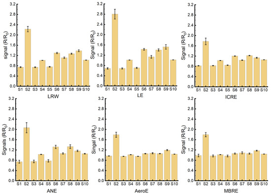
Figure 2.
The means and standard deviations of the e-nose sensor signals for each leachate sample.
The Pearson correlations between e-nose sensor signals are displayed in Figure 3. The 10 sensors showed different correlations. S1 had high correlations (positive or negative) with S2, S3, S5, S6, and S8. S1 had high correlations with S1, S2, S3, S5, S6, S7, S8, and S9. These correlations were observed frequently among the e-nose sensors, suggesting that the headspace gas information could be detected by all sensors but may have overlapped. It’s important to have varied cross-sensitivity within a sensor array, and these findings indicate that e-nose technology is capable of discriminating leachate samples. To make better use of e-nose data, signals should be reduced to extract valid information.
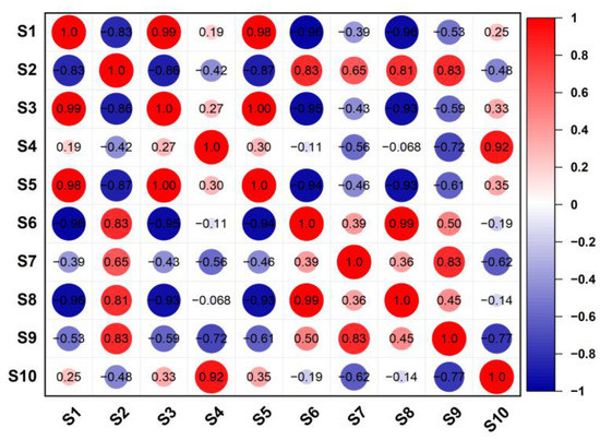
Figure 3.
Sensor signal correlations based on Spearman’s correlations. The color scale denotes the correlations, with 1 indicating a positive correlation (red) and −1 indicating a negative correlation (blue).
3.2. Data Reduction Based on PCA and TSNE
Data reduction can be used to aggregate original data into a representative subset of data or transform them into a more compact representation [24]. Here, PCA was applied to reduce the size and the complexity of the original e-nose dataset while preserving as much information as possible [25]. By converting the original e-nose data into a new linear combination of variables set as principal components (PCs), we used PCA to extract a new dataset with variables orthogonal to each other. To assess the performance of the PCA, the accumulative variance of the variables was applied. Then, the variance of each PC was set as the feature importance, as displayed in Figure 4a. The accumulative variance of the first three PCs was more than 85% in total variance. Figure 4b shows the distribution of 144 samples in three dimensions. Those clusters (LRW, LE, ICRE, and ANE) were clearly separated from each other. The borders between Aero and MBRE were not well-defined, with some samples completely overlapped. This might imply that the headspace gases in the AeroE and MBRE samples were very similar.
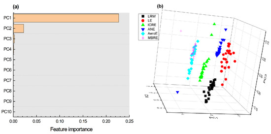
Figure 4.
Visualization of e-nose data dimensionality reduction based on PCA: (a) feature importance according to variance; (b) sample distribution based on the first three PCs.
As a dimensionality reduction technique used to visualize high-dimensional data, TSNE has been successfully applied to e-nose data. By reducing the high-dimensional e-nose data (10 dimensions) into a lower-dimensional space, the samples in this study could be easily visualized in three-dimensional space. Here, TNSE ran for a fixed number of iterations determined by the loss value, with each iteration improving the alignment between the high-dimensional and low-dimensional probability distributions. When the iteration number reached 120, the loss value was not optimized; see Figure 5a. Therefore, the iteration number was set to 120 for e-nose data. As seen in Figure 5b, those clusters (LRW, LE, ICRE, and ANE) were clearly separated from each other and more gathered compared with the PCA results shown in Figure 4b. Similar phenomena can be seen in Figure 5b in that the borders between Aero and MBRE were not well-defined, with some samples totally overlapped.
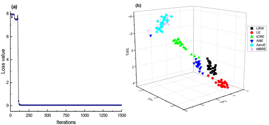
Figure 5.
Visualization of e-nose data dimensionality reduction based on TNSE: (a) the loss value according to iteration; (b) sample distribution based on the first three TPs.
3.3. Leachate Chemical Characterization
Leachate characterization is highly variable and heterogeneous. In this study, the chemical characteristics of incineration leachate, including pH, COD, and ammonia nitrogen, were detected. Table 2 shows the chemical parameter results of six procedures with statistically significant differences (Turkey HSD, p < 0.05). The pH value varied from 8.29 to 6.45, and the changes were not very regular. The changes in COD and ammonia nitrogen were very noticeable, with LE showing the highest values (33,860 mg/L for COD and 2472 mg/L for ammonia nitrogen) and MBRE showing the lowest values (361.2 mg/L for COD and 7.44 mg/L for ammonia nitrogen). The conversion of LRW to MBRE resulted in a COD removal efficiency of 97.71%, which was higher than the maximum removal efficiency (63.59%) achieved with the contaminant coagulation treatment process [4]. The procedure used in this study achieved a high ammonia nitrogen removal efficiency of 99.34%, which was higher than the 98.98% removal efficiency previously obtained with a spacer tube reverse osmosis membrane [26].
Table 2.
Average values of leachate chemical parameters.
Significantly, the chemical parameters of the LE reached their highest (COD and ammonia nitrogen) or lowest (pH) values because during this procedure, the incineration leachate was concentrated. The processed leachate was discharged into a municipal pipe network with chemical parameters that were up to standard.
3.4. Microbial Community Composition and Functional Potential Prediction
The microbial communities in the waste incineration leachate were assessed in terms of amplified 16S rDNA fragments. This type of data is commonly generated through the DNA sequencing of bacterial communities, where the relative abundance of different bacterial taxa can be inferred based on the number of sequencing reads corresponding to each taxon. The profiles of the bacterial communities were complex, and the data revealed that there was a high degree of variation between samples. Table 3 displays the respective phylum- and genus-level abundances of microbial communities. In the leachate samples, Proteobacteria, Firmicutes, and Bacteroidetes were the top three phyla, accounting for more than 90% abundance of the total bacterial community. These findings were similar to those described in previous investigations of fresh incineration leachate [27]. Notably, the relative content (but not absolute content) of Proteobacteria increased with the changing processing procedures. On the contrary, the relative contents of Firmicutes and Bacteroidetes decreased with the changing processing procedures. The microbial communities in the processed leachate were established as meeting the required standards before being released into the municipal pipe network.
Table 3.
Bacterial taxonomic identification and relative abundances at the phylum level in each leachate sample at different water outlets.
Using PICRUSt 2 and the KEGG database (https://www.arb-silva.de/, version: silva_132), metabolic pathways were predicted to determine the functional composition associated with leachate samples, as shown in Figure 6. The analysis of the functional gene families involved categorizing them into various groups that included metabolism, genetic information processing, cellular processes, environmental information processing, organismal systems, and human diseases. Metabolism emerged as the top-performing pathway among these categories, as it was responsible for more than 85% of the total abundances. The dominant level 2 metabolism pathways were the metabolisms of cofactors and vitamins (13.5–15.3%), carbohydrate metabolism (13.2–14.1%), amino acid metabolism (13.7–14.9), metabolisms of terpenoids and polyketides (11.3–12.5%), and metabolisms of other amino acids (7.8–10.2%). These results indicated high bacterial activity. Human disease-related pathways were uncommon. Environmental information processing pathways included signal transduction (0.8–1.9%) and membrane transport (1.1–2.3%).
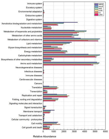
Figure 6.
Prediction of community functional potential (percentage per million functional units) for six leachate samples (LRW, LE, ICRE, ANE, AeroE, and MBRE) based on the KEGG database.
3.5. Recognition Based on E-Nose Data
3.5.1. Monitoring Based on Random Forest
In this study, the area under the curve (AUC) and receiver operator characteristic (ROC) curves were applied to evaluate the performance of the classification models. A high AUC score indicated that the model had a good balance between the true positive rate (TPR) and the false positive rate (FPR), meaning that it could accurately distinguish samples and be useful for the monitoring task. The closer the AUC score was to 1, the closer the model could achieve perfect classification. As shown in Figure 7(a1,b1,c1), the AUC scores for the RF models based on the original e-nose data, PCA-processed e-nose data, and TNSE-processed data were 0.9926, 0.998, and 0.998, respectively. Thus, the RF models could successfully classify the six leachate samples. To further analyze the classification results, ROC curves were used to organize classifiers and visualize the results. In the ROC graphs, the closer the curve is to the (0, 1) point, the better the performance of the classifier. As seen in Figure 7(a2,b2,c2), the classification accuracies for each leachate sample were very different for the training set. Regarding the RF models, the classification model based on TNSE showed a higher accuracy than models based on original data and data processed with PCA. Models based on original data and data processed with PCA misclassified samples for each class, and models based on TNSE only misclassified ANE and MBRE samples, possibly because the ANE and MBRE classes overlapped (as seen in Figure 4a) and the headspace gases of the ANE and MBRE samples were very similar, resulting in models that were difficult to classify.
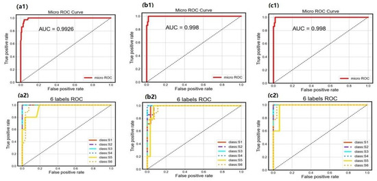
Figure 7.
The evaluation of RF classification based on different datasets: (a1) AUC based on the original data, (b1) AUC based on the PCA data, and (c1) AUC based on the TNSE data; (a2) ROC curve based on the original data, (b2) ROC curve based on the PCA data, and (c2) ROC curve based on the TNSE data. Class S1 refers to LRW, class S2 refers to LE, class S3 refers to ICRE, class S4 refers to AeroE, class S5 refers to ANE, and class S6 refers to MBRE.
To ensure accurate classification performance, testing datasets were used, and each model was run 100 times to reduce the impact of volatility. The average results are displayed in Table 4. The classification model based on TNSE-RF had the best performance, with 99.49% accuracy for the training set and 97.36% accuracy for the testing set, suggesting that the TNSE-RF model had a more stable robustness than the original-RF and PCA-RF models.
Table 4.
The classification results for the training and testing sets based on RF models (100 times).
3.5.2. Monitoring Based on Gradient-Boosted Decision Tree
According to the AUC graphs shown in Figure 8(a1,b1,c1), the best classification result was achieved by the PCA-GBDT model, with an AUC value of 0.9995. The models based on original-GBDT and TNSE-GBDT did not exhibit performance levels that were comparable to the models based on original-RF and TNSE-RF, as shown in Figure 7(a1,c1). As shown in Figure 8(a2,b2,c2), the classification accuracy rates of the RF models were very different. The PCA-GBDT model showed the best accuracy among all models (original-RF, PCA-RF, TNSE-RF, original-GBDT, and TNSE-RF), with no samples misclassified. The models based on original-GBDT and TNSE-RF misclassified samples at different levels.
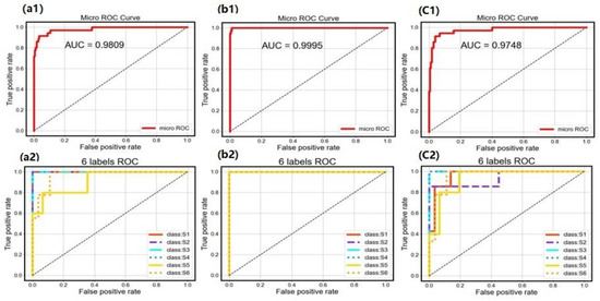
Figure 8.
Evaluation of GBDT classification based on different datasets: (a1) AUC based on the original data, (b1) AUC based on the PCA data, and (c1) AUC based on the TNSE data; (a2) ROC curve based on the original data, (b2) ROC curve based on the PCA data, and (c2) ROC curve based on the TNSE data. Class S1 refers to LRW, class S2 refers to LE, class S3 refers to ICRE, class S4 refers to AeroE, class S5 refers to ANE, and class S6 refers to MBRE.
The GBDT models were run 100 times to decrease their instability, and the classification results of the training and testing data are displayed in Table 5. The results suggest that the PCA-GBDT model had excellent classification performance, achieving 100% accuracy for the training set and 98.92% accuracy for the testing set. As summarized in Table 4 and Table 5, the PCA-GBDT models showed satisfying performance for both the training and the testing datasets, with no overfitting in the modeling.
Table 5.
The classification results for the training and testing sets based on GBDT models.
3.6. Prediction Results of Chemical Parameters and Microbial Community Contents Based on E-Nose Data
3.6.1. Prediction Results of Chemical Parameters and Microbial Community Contents Based on RF
An RF is considered a powerful and flexible tool for predicting continuous numerical values. While modeling, multiple CARTs are trained on different subsets of training data using random selection (bagging and boosting), helping to reduce model variance and overfitting while making the model more robust to noise in the data. In this study, the number of CARTs was set to 35 according to the R2 and MSE values. As with the classification procedure, the prediction models were run 100 times to reduce volatility. The average R2 and MSE values for the prediction RF models based on the original e-nose dataset, the PCA-processed dataset, and the TNSE dataset are displayed in Table 6, Table 7 and Table 8, respectively.
Table 6.
Comparison of the RF prediction models based on the original e-nose dataset.
Table 7.
Comparison of the RF prediction models based on PCA.
Table 8.
Comparison of the RF prediction models based on TSNE.
The e-nose signals provided complete information on leachate headspace gas, which predominantly contained volatile organic compounds such as hydrogen sulfide, methyl mercaptan, acetylene, and other similar compounds. The results of the testing data were not as good as those of the training data because the model was applied to new, unseen data that may have had different characteristics or distributions. The other reason why the data were different between the training and testing datasets was the concept of overfitting, which could have led to poor generalization performance. The overall performance of the training dataset was better than that of the testing dataset, but the results of the testing dataset were not bad, with R2 > 0.80, which was acceptable.
Regarding microbial community composition, the relative contents of Proteobacteria, Firmicutes, and Bacteroidetes were predicted by the RF models. For the training dataset, the three models (original-RF, PCA-RF, and TNSE-RF) were able to predict the contents of microbial community composition well, with R2 values of over 0.96. However, the predictive ability of the RF models for the testing set was inferior to that for the training set. For Proteobacteria, the PCA-RF model demonstrated good predictive power, with an R2 of 0.9768 and an MSE of 0.0025 for the training set and an R2 of 0.8535 and an MSE of 0.0158 for the testing set. For Firmicutes, the original-RF model exhibited strong predictive ability, achieving an R2 value of 0.9947 and an MSE value of 0.0006 for the training set and an R2 value of 0.9651 and an MSE value of 0.0034 for the testing set. The original-RF model showed excellent predictive performance for Bacteroidetes, with an R2 value of 0.9831 and an MSE value of 0.0004 for the training set and an R2 value of 0.8972 and an MSE value of 0.0022 for the testing set. As seen in Table 6, Table 7 and Table 8, the TSNE-RF models outperformed the original-RF model and the PCA-RF model for each parameter in the continuous numerical prediction of chemical parameters.
3.6.2. Prediction Results of Chemical Parameters and Microbial Community Content Results Based on GBDT
A GBDT works by iteratively adding decision trees to an ensemble, with each tree attempting to correct the errors of previous trees. This process is repeated until a stopping criterion, such as the maximum number of trees or a minimum improvement in performance, is met. In this study, a loss function was chosen to stop the modeling. As with the RF modeling, the GBDT prediction models were run 100 times to reduce volatility. The average R2 and MSE values for the prediction RF models based on the original e-nose dataset, the PCA-processed dataset, and the TNSE dataset are displayed in Table 9, Table 10 and Table 11, respectively.
Table 9.
Comparison of the GBDT prediction models based on the original e-nose dataset.
Table 10.
Comparison of the GBDT prediction models based on PCA.
Table 11.
Comparison of the GBDT prediction models based on TNSE.
As can be observed in Table 6, Table 7, Table 8, Table 9, Table 10 and Table 11, the GBDT models overall performed better than the RF models. The PCA-GBDT models demonstrated superior performance in predicting microbial community composition, achieving R2 values above 0.99 and MSE values below 0.0003 (due to the use of relative contents for three microbial communities) for the training set and R2 values exceeding 0.86 and MSE values below 0.015 for the testing set. The original-GBDT models exhibited exceptional performance in forecasting microbial community composition, with R2 values surpassing 0.99 for the training dataset and 0.86 for the testing dataset.
4. Conclusions
Waste incineration is one of the most effective methods for waste disposal, with advantages of waste volume reduction, waste-to-energy benefits, reductions in greenhouse gas emissions, and land saving. This study applied e-nose technology to detect the headspace gas of incineration leachate and to assess the relationship among e-nose signals, chemical characterization, and microorganism changes. Some conclusions can be drawn:
- (1).
- The chemical parameter results in six studied procedures showed statistically significant differences. Proteobacteria, Firmicutes, and Bacteroidetes were the top three phyla, accounting for more than 90% abundance of the total bacterial community.
- (2).
- The changes in the headspace gas of the leachate samples were detected with e-nose sensors. The information in the e-nose sensor signals overlapped according to Pearson correlations. PCA and TNSE were applied to extract valid e-nose information. According to three-dimensional plots, the borders between the Aero and MBRE samples were not well-defined, with some samples totally overlapped in both PCA and TNSE.
- (3).
- RF and GBDT models were applied to assess the relationship among e-nose signals of the leachate headspace gas, chemical parameter changes, and microorganism changes with PCA and TNSE. The PCA-GBDT models showed satisfying performance for both the training data (100% accuracy) and the testing data (98.92% accuracy), with no overfitting in the modeling. Regarding numerical prediction, the GBDT models performed better than the RF models in this study. The original-GBDT models exhibited exceptional performance in forecasting chemical parameter changes, with R2 values surpassing 0.99 for the training dataset and 0.86 for the testing dataset. The PCA-GBDT models demonstrated superior performance in predicting microbial community composition, achieving R2 values above 0.99 and MSE values below 0.0003 for the training set and R2 values exceeding 0.86 and MSE values below 0.015 for the testing set.
Up until now, there have been few in depth studies conducted to gather information regarding headspace gas, chemical parameters, and microorganism changes in leachate samples. This research offers a more efficient monitoring method for the effective enforcement and implementation of monitoring programs by utilizing e-nose technology combined with machine learning to provide more valuable insights compared with traditional instrumental measurements.
Author Contributions
Conceptualization, S.Q. and J.Z.; Data curation, Z.Z.; Formal analysis, J.H.; Funding acquisition, S.Q.; Methodology, Z.Z. and J.H.; Resources, S.Q.; Software, Q.Z.; Validation, Q.Z.; Writing—original draft, S.Q.; Writing—review and editing, S.Q.; Investigation, J.Z.; Supervision, J.Z. All authors have read and agreed to the published version of the manuscript.
Funding
The research was funded by the National Key R&D Program of China (2019YFE0124600), and the Key Research and Development Program of Zhejiang Province, China (No. 2023C03134).
Institutional Review Board Statement
Not applicable.
Informed Consent Statement
Not applicable.
Data Availability Statement
Data available on request due to restrictions e.g., privacy or ethical. The data presented in this study are available on request from the corresponding author. The data are not publicly available due to the company policy.
Conflicts of Interest
The authors declare no conflict of interest.
References
- Chen, W.; He, C.; Zhuo, X.; Wang, F.; Li, Q. Comprehensive evaluation of dissolved organic matter molecular transformation in municipal solid waste incineration leachate. Chem. Eng. J. 2020, 400, 126003. [Google Scholar] [CrossRef]
- Jiao, F.; Zhang, L.; Dong, Z.; Namioka, T.; Yamada, N.; Ninomiya, Y. Study on the species of heavy metals in MSW incineration fly ash and their leaching behavior. Fuel Process. Technol. 2016, 152, 108–115. [Google Scholar] [CrossRef]
- Fu, Z.; Lin, S.; Tian, H.; Hao, Y.; Wu, B.; Liu, S.; Luo, L.; Bai, X.; Guo, Z.; Lv, Y. A comprehensive emission inventory of hazardous air pollutants from municipal solid waste incineration in China. Sci. Total Environ. 2022, 826, 154212. [Google Scholar] [CrossRef]
- Ren, X.; Xu, X.; Xiao, Y.; Chen, W.; Song, K. Effective removal by coagulation of contaminants in concentrated leachate from municipal solid waste incineration power plants. Sci. Total Environ. 2019, 685, 392–400. [Google Scholar] [CrossRef] [PubMed]
- Jiang, F.; Qiu, B.; Sun, D. Degradation of refractory organics from biologically treated incineration leachate by VUV/O3. Chem. Eng. J. 2019, 370, 346–353. [Google Scholar] [CrossRef]
- Shi, J.; Sun, D.; Dang, Y.; Qu, D. Characterizing the degradation of refractory organics from incineration leachate membrane concentrate by VUV/O3. Chem. Eng. J. 2022, 428, 132281. [Google Scholar] [CrossRef]
- Funari, V.; Gomes, H.I.; Cappelletti, M.; Fedi, S.; Dinelli, E.; Rogerson, M.; Mayes, W.M.; Rovere, M. Optimization Routes for the Bioleaching of MSWI Fly and Bottom Ashes Using Microorganisms Collected from a Natural System. Waste Biomass Valorization 2019, 10, 3833–3842. [Google Scholar] [CrossRef]
- Anand, U.; Li, X.; Sunita, K.; Lokhandwala, S.; Gautam, P.; Suresh, S.; Sarma, H.; Vellingiri, B.; Dey, A.; Bontempi, E.; et al. SARS-CoV-2 and other pathogens in municipal wastewater, landfill leachate, and solid waste: A review about virus surveillance, infectivity, and inactivation. Environ. Res. 2022, 203, 111839. [Google Scholar] [CrossRef]
- Wijaya, D.R.; Afianti, F.; Arifianto, A.; Rahmawati, D.; Kodogiannis, V.S. Ensemble machine learning approach for electronic nose signal processing. Sens. Bio-Sens. Res. 2022, 36, 100495. [Google Scholar] [CrossRef]
- John, A.T.; Murugappan, K.; Nisbet, D.R.; Tricoli, A. An Outlook of Recent Advances in Chemiresistive Sensor-Based Electronic Nose Systems for Food Quality and Environmental Monitoring. Sensors 2021, 21, 2271. [Google Scholar] [CrossRef]
- Gonzalez Viejo, C.; Fuentes, S. Digital Assessment and Classification of Wine Faults Using a Low-Cost Electronic Nose, Near-Infrared Spectroscopy and Machine Learning Modelling. Sensors 2022, 22, 2303. [Google Scholar] [CrossRef]
- Kaushal, S.; Nayi, P.; Rahadian, D.; Chen, H.-H. Applications of Electronic Nose Coupled with Statistical and Intelligent Pattern Recognition Techniques for Monitoring Tea Quality: A Review. Agriculture 2022, 12, 1359. [Google Scholar] [CrossRef]
- Yakubu, H.G.; Kovacs, Z.; Toth, T.; Bazar, G. Trends in artificial aroma sensing by means of electronic nose technologies to advance dairy production—A review. Crit. Rev. Food Sci. Nutr. 2023, 63, 234–248. [Google Scholar] [CrossRef]
- Gao, M.; Yang, J.; Li, S.; Liu, S.; Xu, X.; Liu, F.; Gu, L. Effects of incineration leachate on anaerobic digestion of excess sludge and the related mechanisms. J. Environ. Manag. 2022, 311, 114831. [Google Scholar] [CrossRef]
- Chen, J.; Wang, Y.; Shao, L.; Lü, F.; Zhang, H.; He, P. In-situ removal of odorous NH3 and H2S by loess modified with biologically stabilized leachate. J. Environ. Manag. 2022, 323, 116248. [Google Scholar] [CrossRef]
- Morley, N.; Baggs, E.M.; Dörsch, P.; Bakken, L. Production of NO, N2O and N2 by extracted soil bacteria, regulation by NO2− and O2 concentrations. FEMS Microbiol. Ecol. 2008, 65, 102–112. [Google Scholar] [CrossRef]
- Canziani, R.; Emondi, V.; Garavaglia, M.; Malpei, F.; Pasinetti, E.; Buttiglieri, G. Effect of oxygen concentration on biological nitrification and microbial kinetics in a cross-flow membrane bioreactor (MBR) and moving-bed biofilm reactor (MBBR) treating old landfill leachate. J. Membr. Sci. 2006, 286, 202–212. [Google Scholar] [CrossRef]
- Chegukrishnamurthi, M.; Shekh, A.; Ravi, S.; Narayana Mudliar, S. Volatile organic compounds involved in the communication of microalgae-bacterial association extracted through Headspace-Solid phase microextraction and confirmed using gas chromatography-mass spectrophotometry. Bioresour. Technol. 2022, 348, 126775. [Google Scholar] [CrossRef]
- Qiu, S.; Hou, P.; Huang, J.; Han, W.; Kang, Z. The Monitoring of Black-Odor River by Electronic Nose with Chemometrics for pH, COD, TN, and TP. Chemosensors 2021, 9, 168. [Google Scholar] [CrossRef]
- HJ 1147-2020; Water Qulity—Determination of pH—Electrode Method. Ministry of Ecology and Environment of the People’s Republic of China: Beijing, China, 2020. Available online: https://max.book118.com/html/2020/1129/8117023002003022.shtm (accessed on 1 November 2022).
- HJ/T 70-2001; High-Chlorine Wastewater—Determination of Chemical Oxygen Demand—Chlorine Emendation Method. Ministry of Ecology and Environment of the People’s Republic of China: Beijing, China, 2001. Available online: https://www.doc88.com/p-9982565679330.html?r=1 (accessed on 1 November 2022).
- HJ 535-2009; Water Quality—Determination of Ammonia Nitrogen—Nessler’s Reagent Spectrophotometry. Ministry of Ecology and Environment of the People’s Republic of China: Beijing, China, 2009. Available online: http://www.doc88.com/p-6836770291709.html (accessed on 1 November 2022).
- Chang, Y.-C.; Chang, K.-H.; Wu, G.-J. Application of eXtreme gradient boosting trees in the construction of credit risk assessment models for financial institutions. Appl. Soft Comput. 2018, 73, 914–920. [Google Scholar] [CrossRef]
- Li, Z.; Yu, J.; Dong, D.; Yao, G.; Wei, G.; He, A.; Wu, H.; Zhu, H.; Huang, Z.; Tang, Z. E-nose based on a high-integrated and low-power metal oxide gas sensor array. Sens. Actuators B Chem. 2023, 380, 133289. [Google Scholar] [CrossRef]
- Avian, C.; Leu, J.-S.; Prakosa, S.W.; Faisal, M. An Improved Classification of Pork Adulteration in Beef Based on Electronic Nose Using Modified Deep Extreme Learning with Principal Component Analysis as Feature Learning. Food Anal. Methods 2022, 15, 3020–3031. [Google Scholar] [CrossRef]
- Ren, X.; Song, K.; Xiao, Y.; Zong, S.; Liu, D. Effective treatment of spacer tube reverse osmosis membrane concentrated leachate from an incineration power plant using coagulation coupled with electrochemical treatment processes. Chemosphere 2020, 244, 125479. [Google Scholar] [CrossRef] [PubMed]
- Gao, Y.; Sun, D.; Dang, Y.; Lei, Y.; Ji, J.; Lv, T.; Bian, R.; Xiao, Z.; Yan, L.; Holmes, D.E. Enhancing biomethanogenic treatment of fresh incineration leachate using single chambered microbial electrolysis cells. Bioresour. Technol. 2017, 231, 129–137. [Google Scholar] [CrossRef] [PubMed]


Disclaimer/Publisher’s Note: The statements, opinions and data contained in all publications are solely those of the individual author(s) and contributor(s) and not of MDPI and/or the editor(s). MDPI and/or the editor(s) disclaim responsibility for any injury to people or property resulting from any ideas, methods, instructions or products referred to in the content. |
© 2023 by the authors. Licensee MDPI, Basel, Switzerland. This article is an open access article distributed under the terms and conditions of the Creative Commons Attribution (CC BY) license (https://creativecommons.org/licenses/by/4.0/).