Simulation of Electrical Biofilm Impedance to Determine the Sensitivity of Electrode Geometries

Abstract

Biofilms are ubiquitous at interfaces of natural and technical origin. Depending on type and application, biofilm formation is desired or has to be prevented. Therefore, reliable detection of initial biofilm growth is essential in many areas. One method of biofilm monitoring is the electrochemical impedance spectroscopy. Among other factors, this method is heavily dependent on the electrode geometry. In order to achieve a high measurement sensitivity, the electrode size must be chosen according to the biofilm that is to be measured. This paper presents an approach for simulating and modeling the optimal electrode geometry for a specific biofilm. First, a geometric model of a biofilm with up to 6000 individual bacteria is generated. The simulated impedances are used to calculate which electrode geometry maximizes sensitivity depending on the biofilm height. In the chosen example of an E. coli biofilm in a nutrient solution, the optimum size of an interdigital electrode (bar gap equals width) was 2.5 µm for a biofilm height of up to 2 µm. The used algorithms and models can be simply adapted for other biofilms. In this way, the most sensitive electrode geometry for a specific biofilm measurement can be determined with minimal effort.

1. Introduction

Biofilms as an association of a wide variety of microorganisms occur ubiquitously on a wide variety of surfaces and change their properties. Examples include the enormous damages caused by corrosion, increased flow resistance, and reduced thermal conductivity. The early detection and elimination of biofilms is therefore of enormous economic importance, especially in industrial plants. To do this, one must look at their special features. In biofilms, the organisms are embedded in a matrix of extracellular polymeric substances (EPSs). This protects them from environmental influences such as high temperatures, extreme pH values, or changing concentrations of inorganic salts and biological and chemical disinfectants [1]. If the interfaces are not sufficiently disinfected/sterilized, the biofilm can increase considerably in size, as the EPS is increasingly formed to serve as a diffusion barrier and protect the bacteria inside the biofilm from external influences.

Biofilms are of particular importance with regard to the resistance issue, as genetic information is exchanged in them by horizontal gene transfer [2]. Early detection of biofilms is becoming increasingly relevant not only for human and veterinary medicine but also for the food industry and water management [3]. Biofilm formation can also cause plant material, such as plastic seals and various types of metal, to decompose [4]. Even higher alloyed materials, such as stainless steel and CrNiMo steel, can be harmed. In Germany alone, damage amounting to EUR 12.5 billion is caused each year by corrosion alone [4]. Around 20% of this is microbiological and is mainly caused by biofouling and biofilm formation.

In order to avoid or at least reduce this damage, early detection of biofilms and their characterization is essential. There are various approaches for biofilm measurement. The classic methods are microbiological cultivation with subsequent isolation of the individual cultures and also microscopic methods. However, these methods require laboratory equipment and time and also do not provide real-time information at the measurement point. This is why intensive research is being carried out on measurement methods for online monitoring of biofilms. This involves the application of various technologies with specific advantages and disadvantages, for example, acoustic surface waves [5], electrochemical impedance spectroscopy (EIS) [6,7], quartz crystal microbalance [8], isothermal microcalorimetry [9], and optical detection [10]. Furthermore, there are electrochemical approaches for biofilm control, such as for controlling adhesion, electrochemical communication, and electrochemical removal [11].

In addition to EIS, several other electrochemical techniques have been developed to monitor biofilm, including chronopotentiometry (CP), chronoamperometry (CA), differential pulse voltammetry (DPV), and cyclic voltammetry (CV). These are preferred methods due to their high sensitivity, exceptional resolution, and rapid response. They are based, among other things, on redox reactions using naturally occurring metabolites in the extracellular matrix of the biofilm or with added redox mediators, e.g., B. methylene blue. The advantage of EIS here is that non-destructive measurements are possible in real-time, independent of any redox mediators. Therefore, EIS is ideal for analyzing biofilm dynamics at different times [12], e.g., the initial formation, the growth, and the responses to environmental changes. 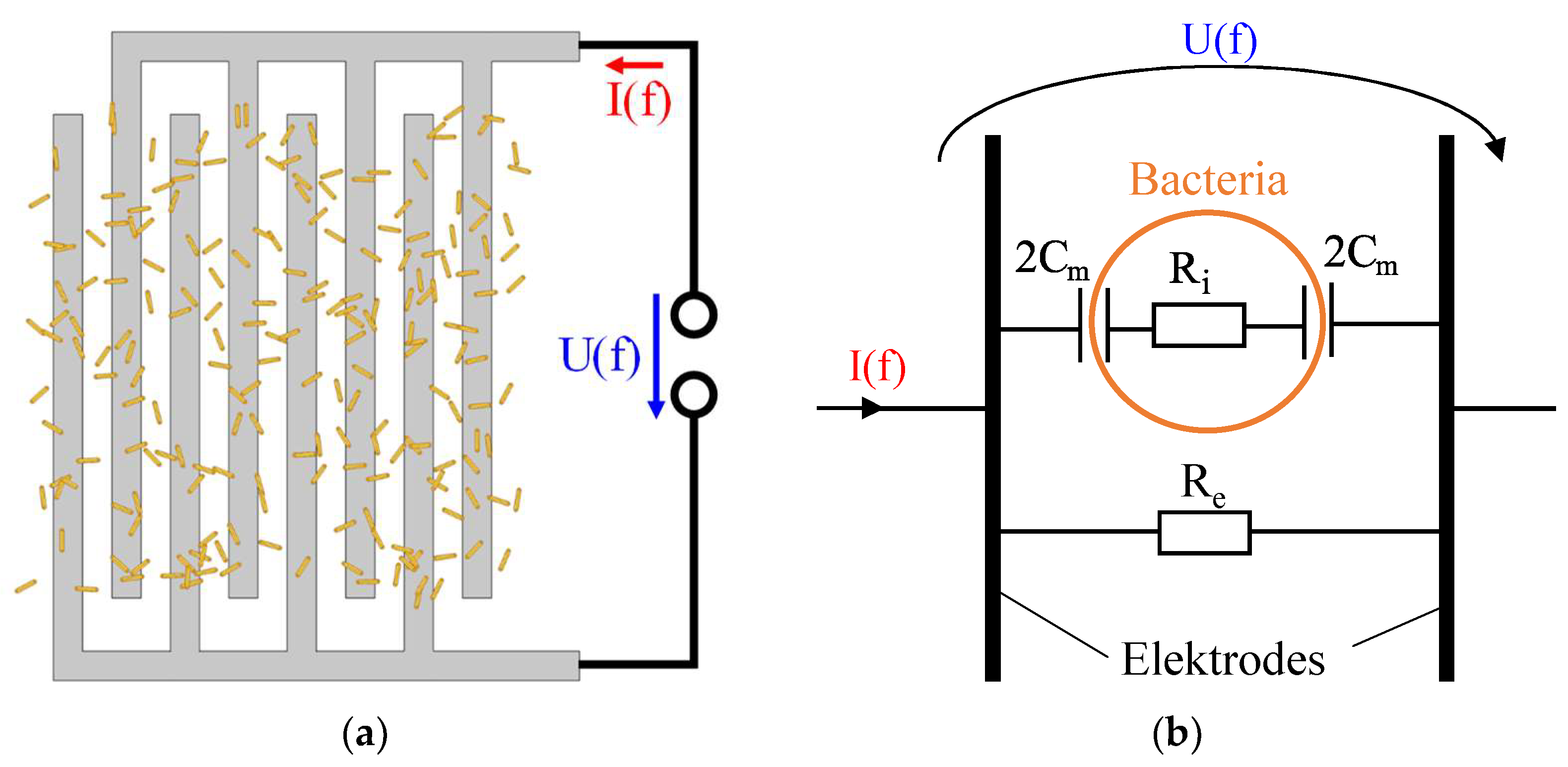As EIS can be implemented with comparatively little equipment, space, and financial outlay, it is also a valuable technique for expanding existing measurement setups [13,14]. This makes EIS a promising measurement method for biofilm monitoring. The electrical impedance, as a quotient of voltage and current, describes the complex, frequency-dependent alternating current resistance of an object. For the measurement, the device under test is stimulated with either a known voltage or a known current and the complementary value is measured. In the case of biofilms, measuring electrodes are placed in contact with a liquid medium in which the growth will take place (Figure 1a). The adhesion of microbes to and around the electrode surface can then be measured as a change in impedance. A simple electrical equivalent circuit diagram of a bacterium consists of the capacitance of the cell membrane C_m, the intracellular resistance R_i, and the extracellular resistance of the medium R_e (Figure 1b). The higher the frequency, the higher the current flow through the cell membrane. Therefore, the characterization of the cell membrane and the protoplasm is only possible at higher frequencies. At low frequencies, C_m has a low conductivity and the measured impedance is mainly determined by the medium. Thus, at low frequencies, the number of bacteria displacing the medium in the electrode area is more accurately measurable.

The results of an impedance measurement depend on a variety of parameters. The most important are stimulation strength (amplitude of current or voltage), excitation waveform (sine, square, etc.), frequency range, environmental noise, electrode geometry, electrode material, measurement medium, temperature, bacterial strain, measurement leads, and electrical properties of the front end. This work focuses on the optimization of the electrode geometry to increase the sensitivity of biofilm growth measurements.

Micro-electrodes for the EIS of biofilms are available on the market in various shapes and sizes. The electrode gaps are usually between 5 µm and 20 µm. The optimum geometry depends on the size, quantity, and electrical properties of the bacteria. This means that a biofilm measurement setup always contains the selection of a suitable electrode, depending on the object to be measured. However, buying or developing different electrode sizes and selecting the best one experimentally is very time-consuming and cost-intensive. It would therefore be advantageous, if it were possible, to calculate in advance which electrode geometry is most sensitive for a specific biofilm.

In general, the higher the change in the measurement signal for a specific change in the measurement object, the higher the sensitivity of a measurement. In classic voltage-controlled impedance measurement, the measured variables are the amplitude and phase of the current. The impedance measurement of biofilm growth starts with the reference impedance $Z_0$ without bacteria. This is the impedance of the front end, supply lines, electrodes, and the surrounding medium. As the biofilm grows, the impedance $Z_{bf}$ changes starting from the reference value. The sensitivity of the impedance measurement for amplitude $S_{abs}$ and phase $S_{pha}$ can therefore be defined as follows:

$$S_{abs}=\frac{\left|Z_{bf}\right|}{\left|Z_0\right|}-1,$$

(1)

$$S_{pha}=\angle {\mathrm{Z}}_{bf}-\angle {\mathrm{Z}}_0$$

(2)

Accordingly, $S_{abs}$ = 0.5, for example, means the absolute value of the impedance has increased by 50% due to the biofilm, compared to the reference impedance without bacteria. The aim of this study is to optimize the electrode geometry in such a way that $S_{abs}$ and $S_{pha}$ are maximized for specific biofilm height.

At the beginning of biofilm growth, the bacteria are scattered and only later form a thin layer. If the focus is on measuring the initial biofilm formation, the measurement must be sensitive to the area near the electrode. Smaller electrode distances are generally more suitable for this. If the electrode distance is too small, much smaller than the bacteria, then the proportion of the current flowing through the bacteria decreases and the sensitivity is lower. For the measurement of biofilms with a higher thickness, correspondingly larger electrode spacing is better. This relationship is illustrated qualitatively in Figure 2. Accordingly, the expected biofilm height must also be taken into account when choosing the electrode size. Hence, the electrode geometry for which the sensitivity is maximized for a certain biofilm height is sought.

One possible theoretical calculation approach is the use of the finite element method (FEM). Mathematical problems that are difficult to solve analytically can be discretized and solved numerically using the FEM. For example, FEM has already been used to determine how the skin impedance changes with different needle electrodes [15]. Another study has already shown how a coplanar waveguide with several bacteria can be simulated using FEM [16]. The FEM has also been used to determine how the skin impedance changes with different needle electrode sizes. For this work, a biofilm with thousands of single bacteria was modeled. The optimum electrode geometry for a specific bacterial strain could be derived from the model.

2. Materials and Methods

2.1. Approach

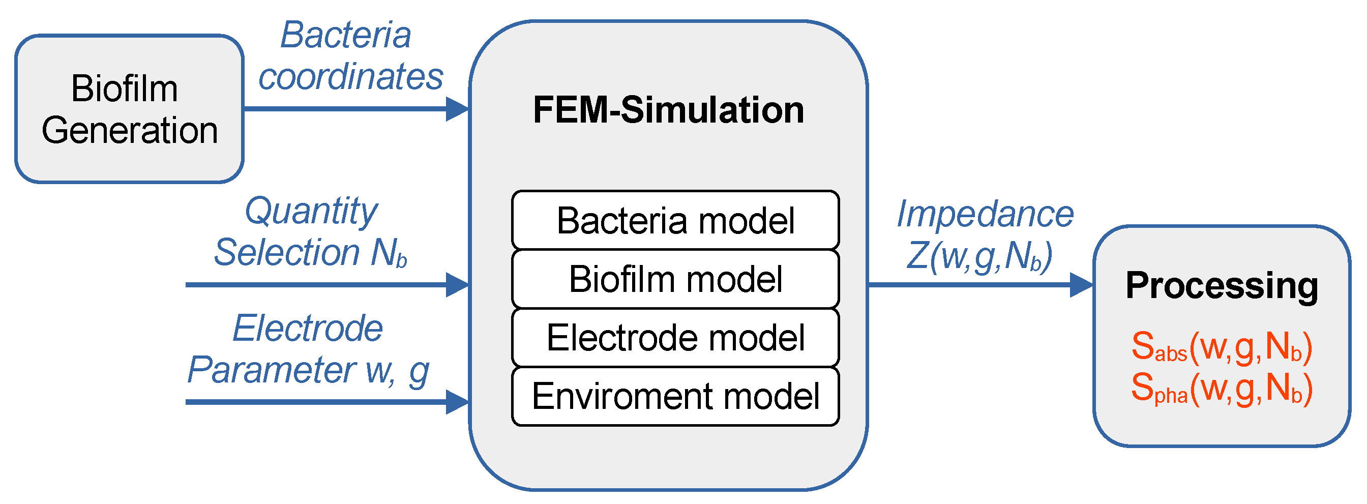
First of all, the geometry of a biofilm with a certain number of bacteria must be generated. In order to simulate how sensitively the growth of this biofilm can be measured with an electrode arrangement, a comprehensive model is required (Figure 3). It must contain the following:

• Geometrically and electrically adequate description of a bacterium;
• Geometric model of a biofilm consisting of a variable number of bacteria;
• The bacteria environment respective to the measuring medium;
• Electrodes with variable geometry and active-electrical properties.

This model is used to calculate the impedance for any combination of electrode geometry and biofilm height. Biofilm growth can be simulated by gradually increasing the number of bacteria in the biofilm. If the impedance is calculated for different growth stages, the result is the dependence of the impedance on the number of bacteria respective to the biofilm height. This can be repeated for different electrode sizes. Finally, the simulated impedances can be used to determine which electrode geometry is most sensitive for each biofilm height.

2.2. Modeling of Bacteria

As the reference for the bacterial model, Escherichia coli (E. coli) was selected, as it is a common species in biofilm research. On average, a bacterium is 3 µm long and has a diameter of 1 µm [17,18]. The electrical impedance of a bacterium is mainly affected by the properties of the cytoplasmic membrane and the protoplasm (see also Figure 1b). Although the membrane is only a few nanometers thick, it has a very low conductivity. The protoplasm, on the other hand, has a high conductivity. The values given in

Table 1. Parameters of the E. coli model for FEM simulation.

Parameter	Symbol	Value	Reference
Bacteria length	lb	3 µm	[17,18]
Bacteria radius	rb	0.5 µm	[17,18]
Membrane thickness	dm	10 nm	[19]
Membrane conductivity	σm	5 × 10−8 S/m	[20]
Protoplasm conductivity	σp	0.17 S/m	[20]
Relative electrical permittivity membrane	εm	9.5	[20]
Relative electrical permittivity protoplasm	εp	67	[20]

were used for the parameters of the bacterial model.

For the FEM simulation, the Electric Currents Interface from Comsol was used. The geometry of the bacterium can easily be created in the shape of a capsule: a cylinder with two semi-spheres at the ends. An outer capsule preserves the electrical properties of the cell membrane. An inner capsule preserves the properties of the protoplasm. The radius of the inner capsule is chosen to be $d_m$ smaller than the radius of the outer capsule $r_b$.

2.3. Modeling of Biofilm

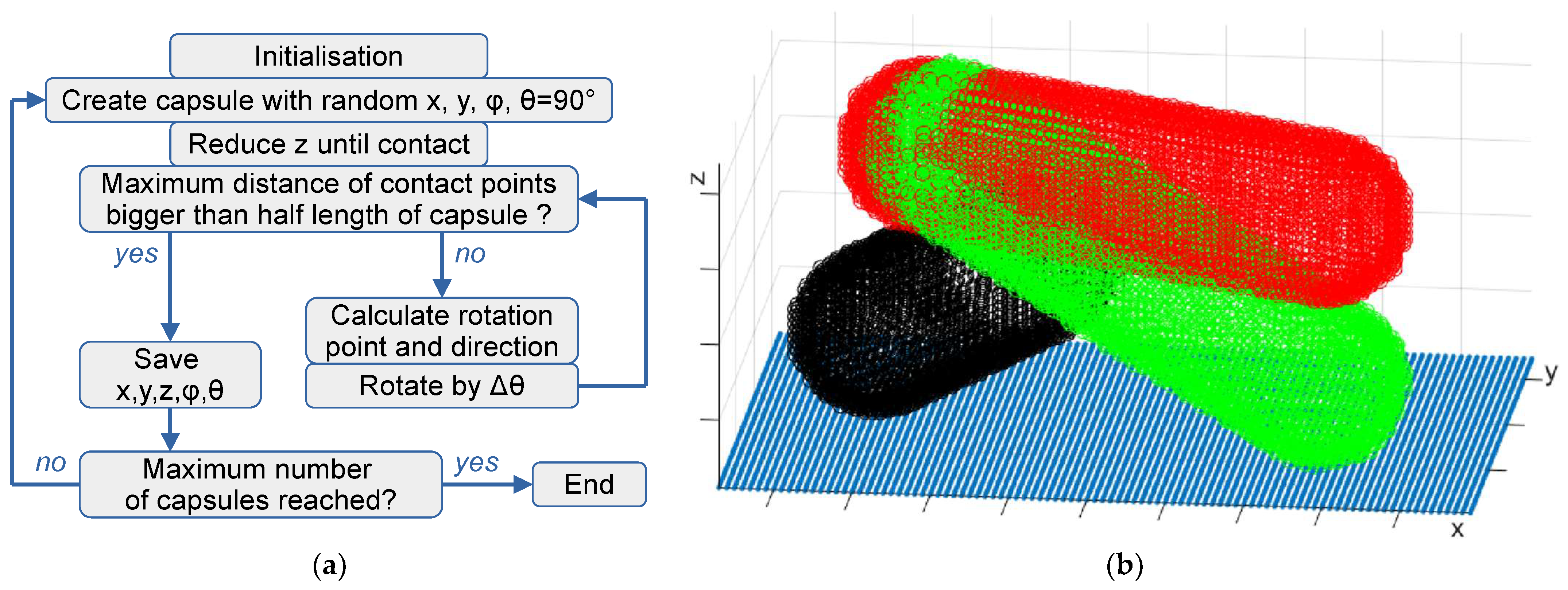
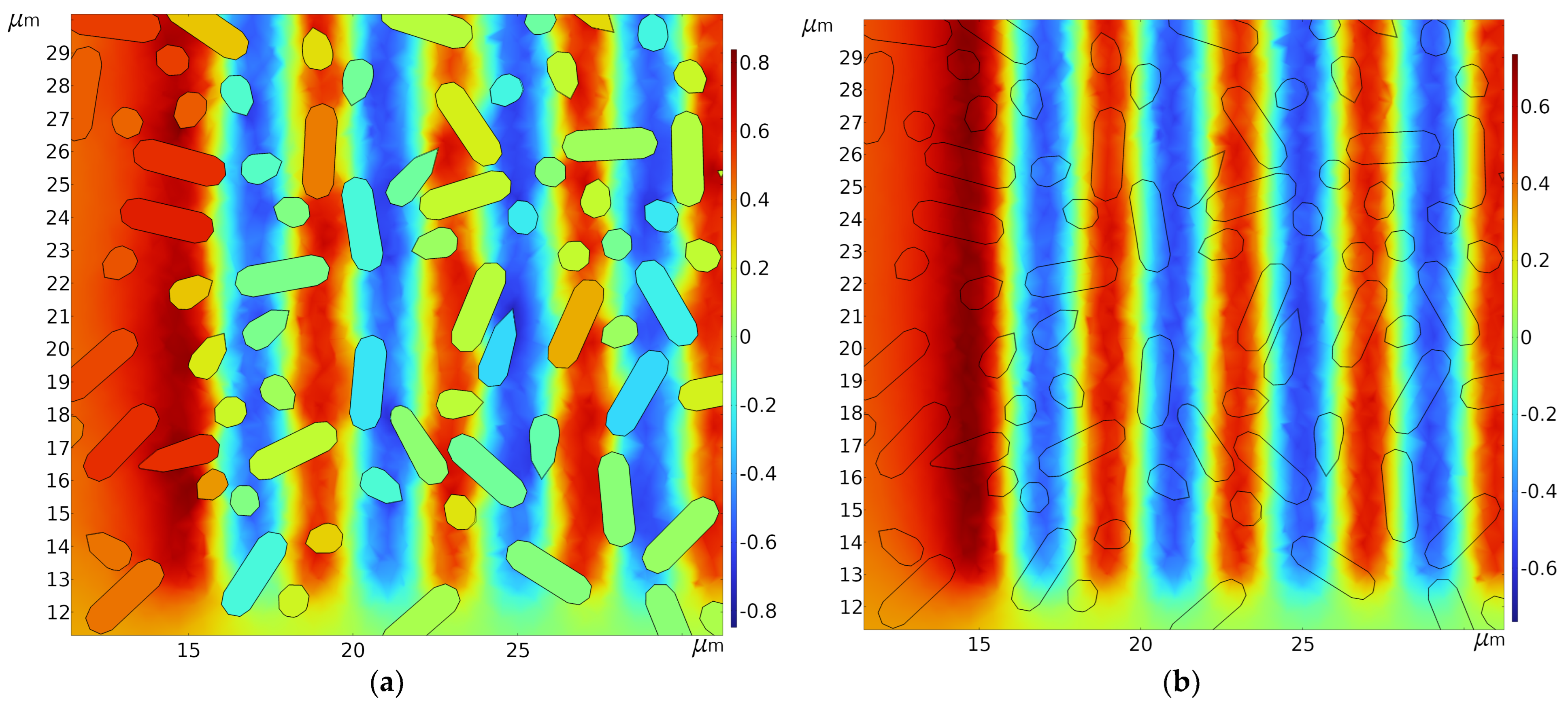
The growth of a biofilm begins with the adhesion of a few bacteria that attach randomly to the surface [3]. As the number of bacteria increases, they lie more on one another, taking on random angles of rotation and filling more and more of the empty spaces until a dense biofilm is formed [21]. Creating hundreds to thousands of capsules manually for the simulation would be too much effort. Therefore, an algorithm was developed with Matlab 2019b that generates a biofilm geometry of variable size.

This algorithm works with the input parameters’ bacterial length $l_b$ and radius $r_b$. In addition, there is the number $N_{b.max}$ of the biofilm capsules to be generated and the length $L_x$ and width $L_y$ of the base area. The algorithm then works iteratively and performs the steps shown in Figure 4 for each capsule to be positioned.

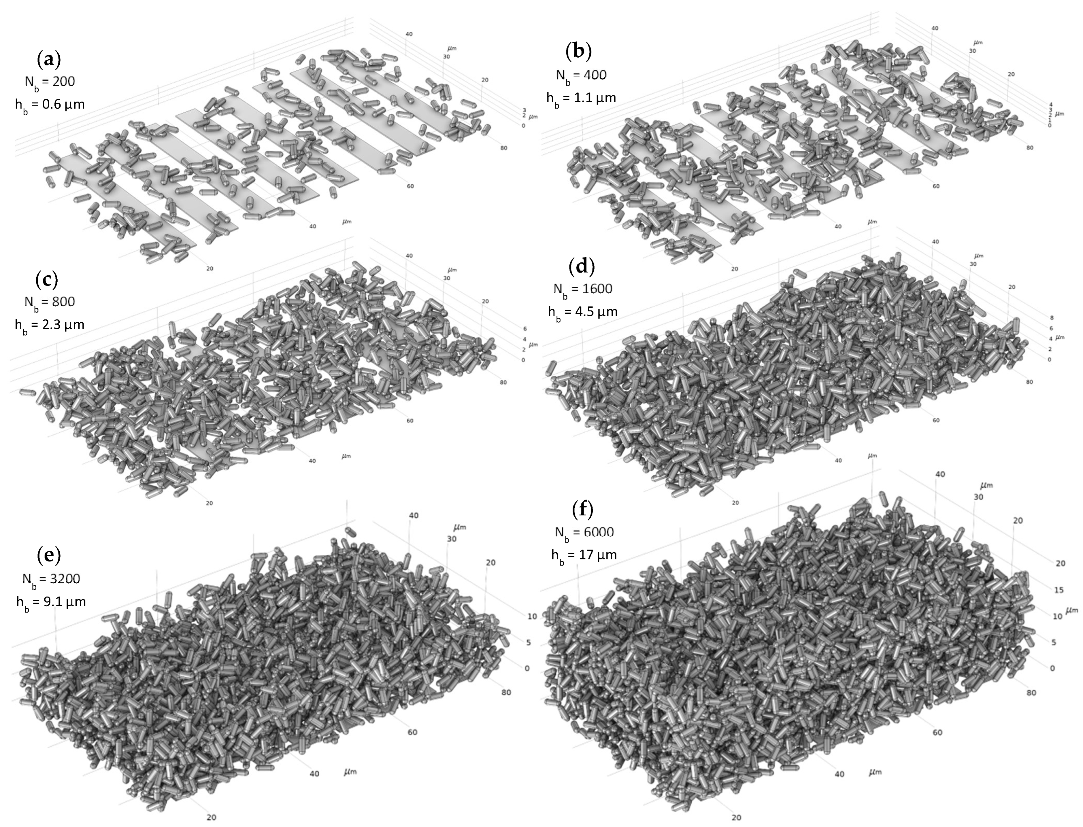
The Matlab algorithm provides a data set with the coordinates and rotations of each individual capsule. This data set is read in by Comsol via a script. This script iteratively creates individual bacteria according to the bacteria model described in Section 2.2 and places them according to the data set of the Matlab algorithm. The number of bacteria to be used for the FEM model can be configured. In this way, a “growing biofilm” can be created step by step (Figure 5). A major advantage of this approach is that any number of biofilms with different parameters can be generated with little effort. For the evaluation, the parameter biofilm height $h_b$ is required. However, in case of a low number of bacteria $N_b$, a height cannot simply be assigned (see Figure 5a). This was handled by determining the height of the biofilm in the configuration with maximum $N_b$. Starting from this maximum height, $h_b$ was then scaled linearly according to the decreasing $N_b$.

In real biofilms, bacteria form an extracellular matrix (EPS). However, the conductivity of the EPS largely corresponds to that of the medium. Furthermore, EPS are transient media for microbial extracellular electron transfer [22]. In the frequency range of interest up to 20 MHz, consequently, there are no structures that would cause a phase shift of the current. For these reasons, the EPS is not expected to influence the optimal electrode geometry, and EPS was not included in the biofilm model to keep the model simple.

2.4. Modeling of Electrodes

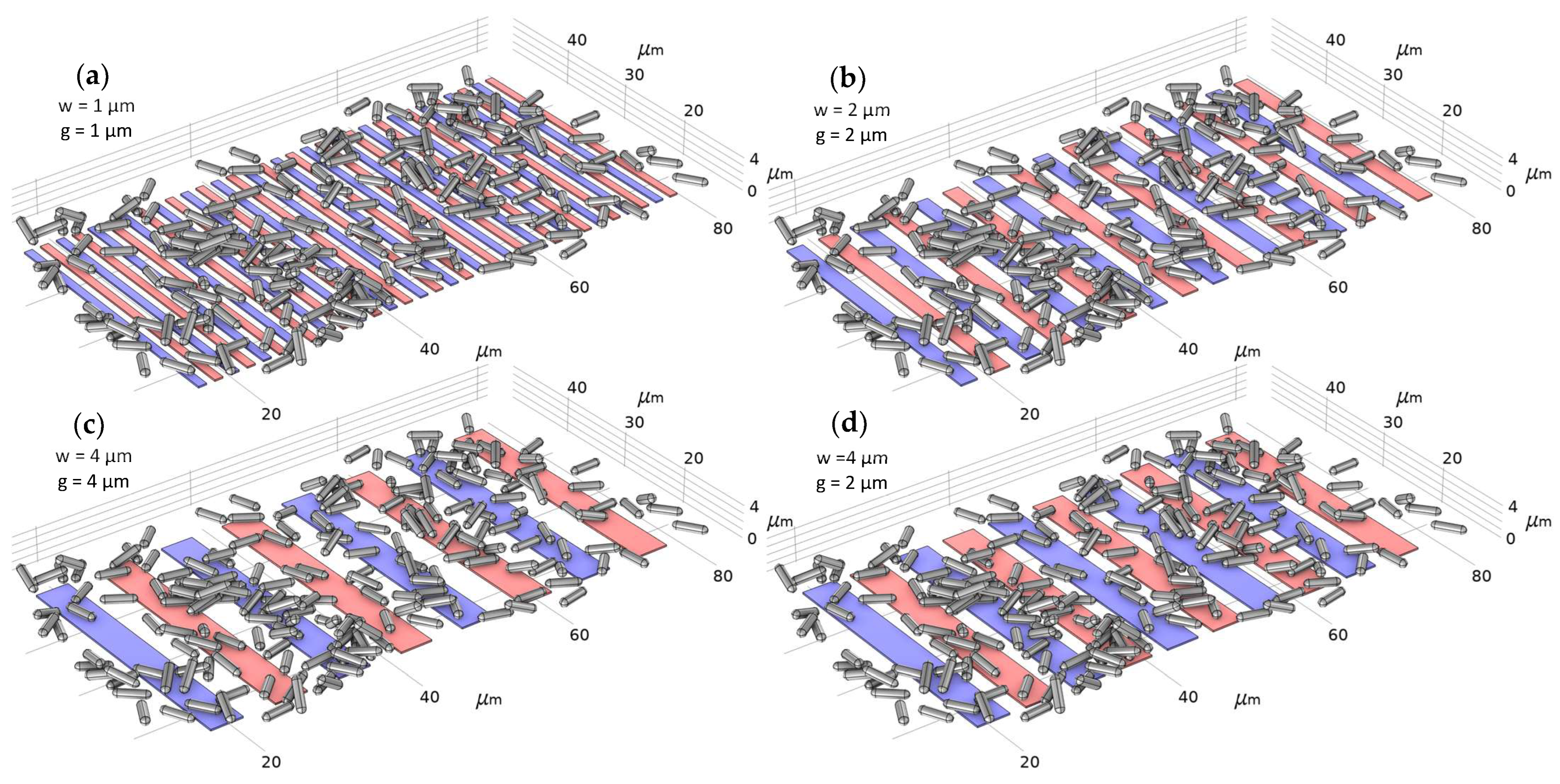
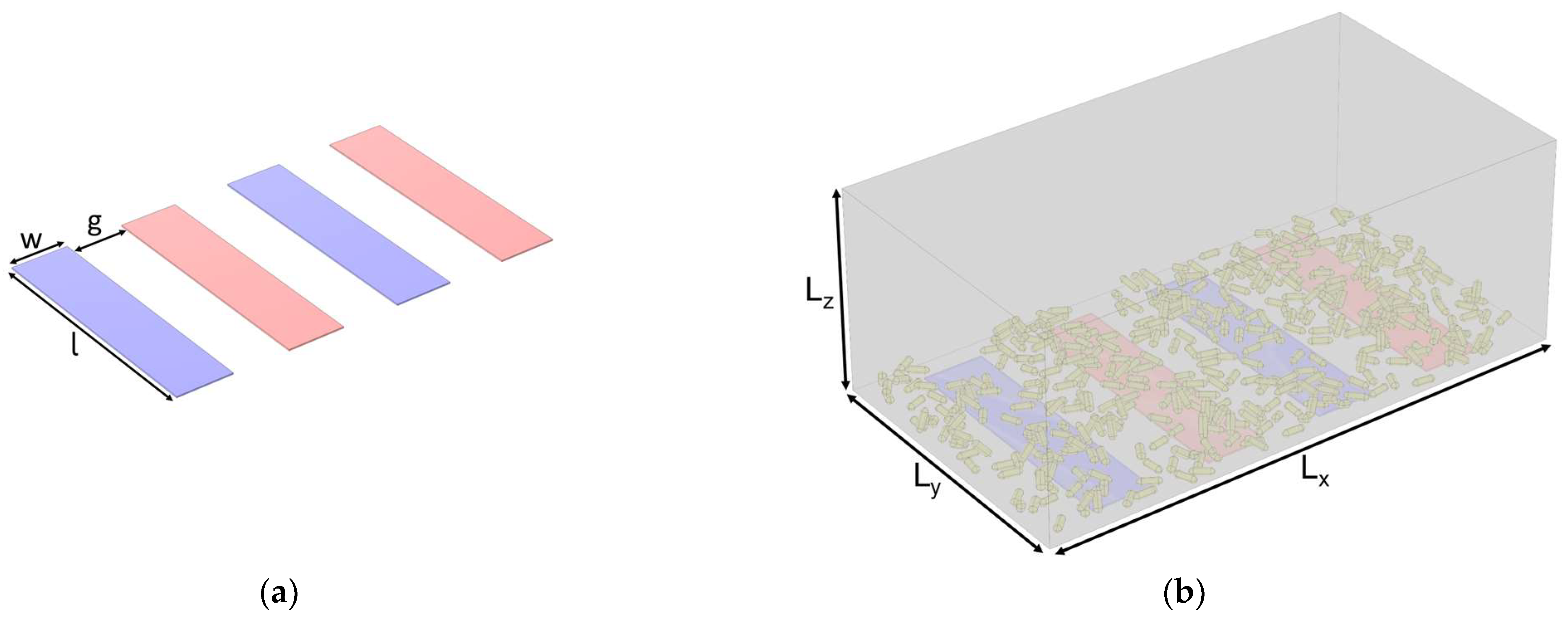
The interdigital electrode (IDE, see Figure 1b) is an established electrode arrangement for the EIS of biofilms. Length $l$, width $w$, gap $g$ and he number of electrode bars determine the operating point of the measurement. The potential is almost constant in the longitudinal direction of the bars (except at the edges). Therefore, the sensitivity of the measurement is mainly dependent on the width $w$ and the gap $g$. The values at which the sensitivity for a specific biofilm reaches its maximum are sought. For this purpose, electrodes with different $w$ and $g$ values are generated. The simulation is then carried out for each electrode size with each growth stage of the biofilm (Figure 6).

A height of 200 nm was chosen for the IDE structure. This is a common value in the production of real IDE in thin-film technology. Since this study focuses on the influence of the geometry on the sensitivity, neither electrochemical effects nor the electrode material should be relevant. For this purpose, the surface of the IDE is generated in the model as an electrically active surface without leads. Every second electrode bar has the same potential. For calculating the impedance, the level of the stimulation voltage is not important in the simulation, as the model does not contain any non-linear components. The voltage was set to 1 V.

2.5. Modeling of Environment and Simulation

In addition to the models for biofilm and electrodes, a specific environment is also required for the simulation. However, the maximum possible number of bacteria, and therefore the size of the environment, is limited by the computing capacity. On the computing cluster used, one simulation run (4 electrode geometries, 10 growth stages up to $N_b$ = 6000, 16 frequencies) required less than one day of computing time. On a PC with a current upper-class CPU with 32 GB RAM and a 500 GB swap file on an SSD hard disk, the simulation took 5 days. The total volume in which the FEM is calculated is a rectangular block with a width of $L_x$ = 72 µm, a depth of $L_y$ = 40 µm, and a height of $L_z$ = 27 µm (Figure 7). The IDE is centered at the bottom of the block, with a bar length of $l$ = 34 µm. The length of the electrode field in the x direction depends on the electrode width, gap, and number of bars, but it is a maximum of 66 µm long. In addition to the simulation environment geometry, electrical properties must also be assigned to it.

In laboratories, biofilms are cultivated in a nutrient medium. In measuring chambers where a medium flows through, the conductivity of the medium remains constant over time. The simulation is designed for this scenario. A frequently used culture medium is LB (lysogeny broth). During cultivation, this usually has a conductivity of ${\sigma }_{LB}$ = 1.2 S/m. This value is used for the environmental conductivity in the simulation. The permittivity corresponds to that of water and is set to ${\epsilon }_{LB}$ = 80.

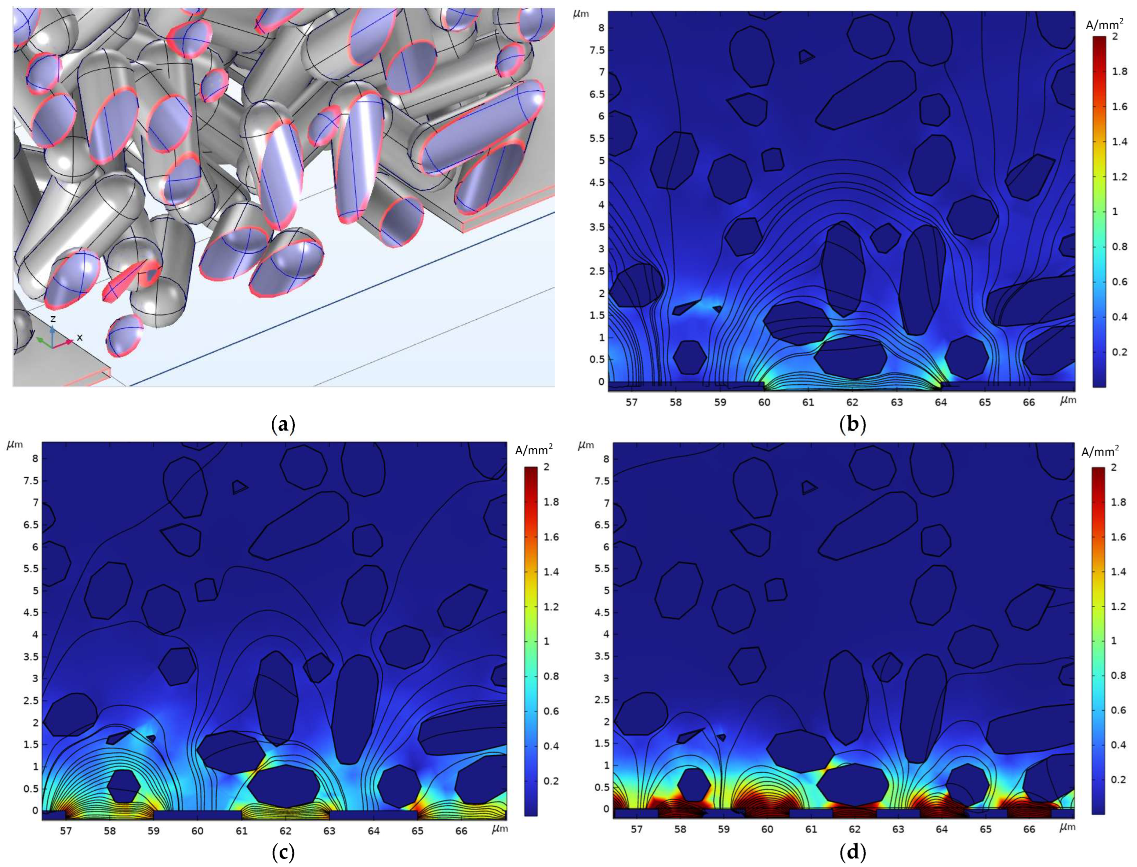
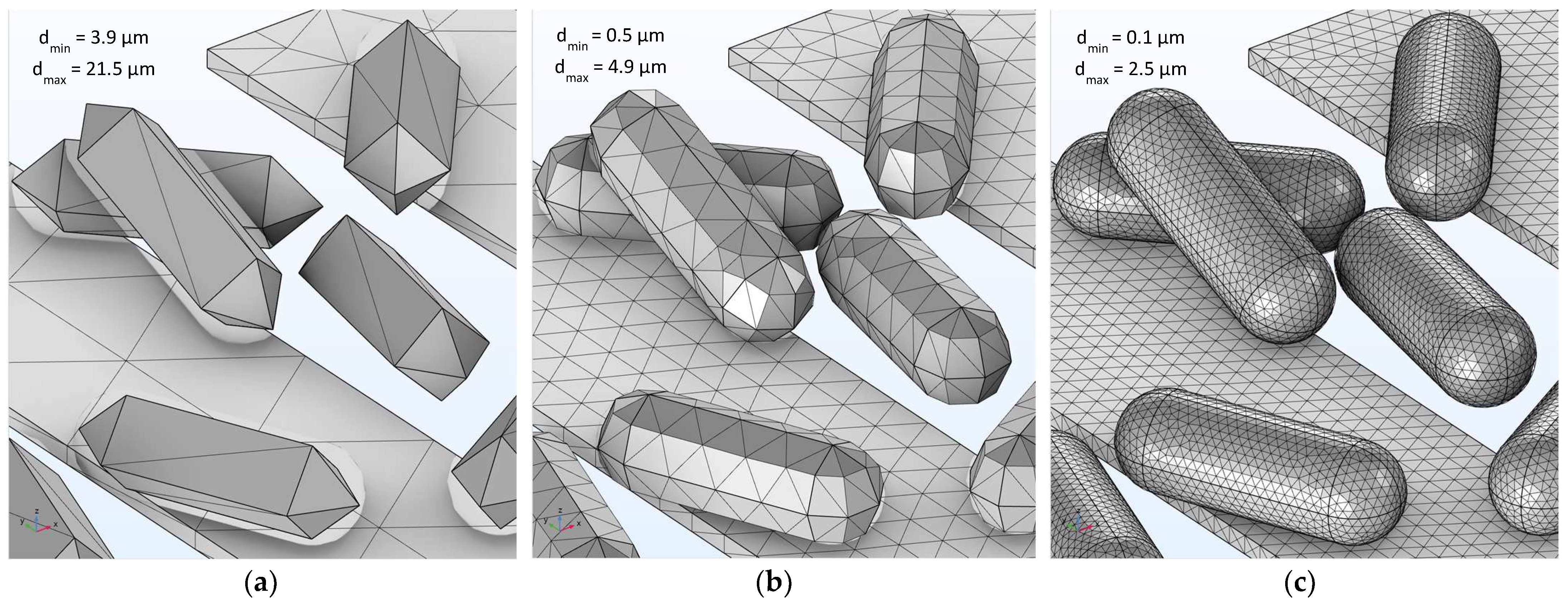
A compromise between quality and computational effort had to be found for the mesh resolution of the FEM simulation (Figure 8). The decisive parameters are the maximum and minimum element size $d_{min}$ and $d_{max}$. Too coarse elements lead to inaccurate simulation results and too fine elements lead to excessive memory requirement and computational effort. A good compromise was found with $d_{min}$ = 0.5 µm and $d_{max}$ = 4.9 µm. It should be noted that $d_{min}$ does not represent the absolute minimum. There are critical exceptional areas (thin membranes, curvatures) where element sizes can take on smaller dimensions.

Finally, in order to calculate the impedance spectrum, the frequency range for the voltage excitation must be selected. Electrochemical effects are not relevant in this simulation. Therefore, the simulation only starts at a lower frequency of 1 kHz. Most impedance analyzers operate in the frequency range up to approx. 100 kHz, some even up to 20 MHz. To cover this range broadly, the upper frequency limit was set to 100 MHz.

The total current is required to calculate the impedance from the results of the FEM simulation. This is done by integrating the current density over the electrode surface. Finally, by sorting the data, one data set is generated, that contains the corresponding impedance $Z\left(f,w,g,h_b\right)$ for each frequency, biofilm height, and electrode geometry.

As the positions of the bacteria in the biofilm are random (see algorithm Figure 4a), the impedance is dependent on the individual position and orientation, especially if the number of bacteria is low. This effect becomes clear if it is assumed that there is only one bacterium. In this case, the impedance change would depend significantly on whether this bacterium is located directly on an electrode or in the gap. The more bacteria there are on a larger electrode surface, the less this effect is visible in the impedance, as a stable mean value is achieved. With the parameters selected for the simulation, this effect should be small. Nevertheless, the influence of the orientation of the individual bacteria in the biofilm should be quantified. Therefore, the algorithm described in Section 2.3. was used to generate several biofilms of identical height, but with different positions of the individual bacteria. Each simulation was carried out with at least three different biofilms in order to be able to specify a standard deviation for the impedances and sensitivities.

3. Results and Discussion

3.1. General Results

In the following, the relationships between impedance, biofilm height, electrode geometry, and frequency will be explained on the basis of some selected results.

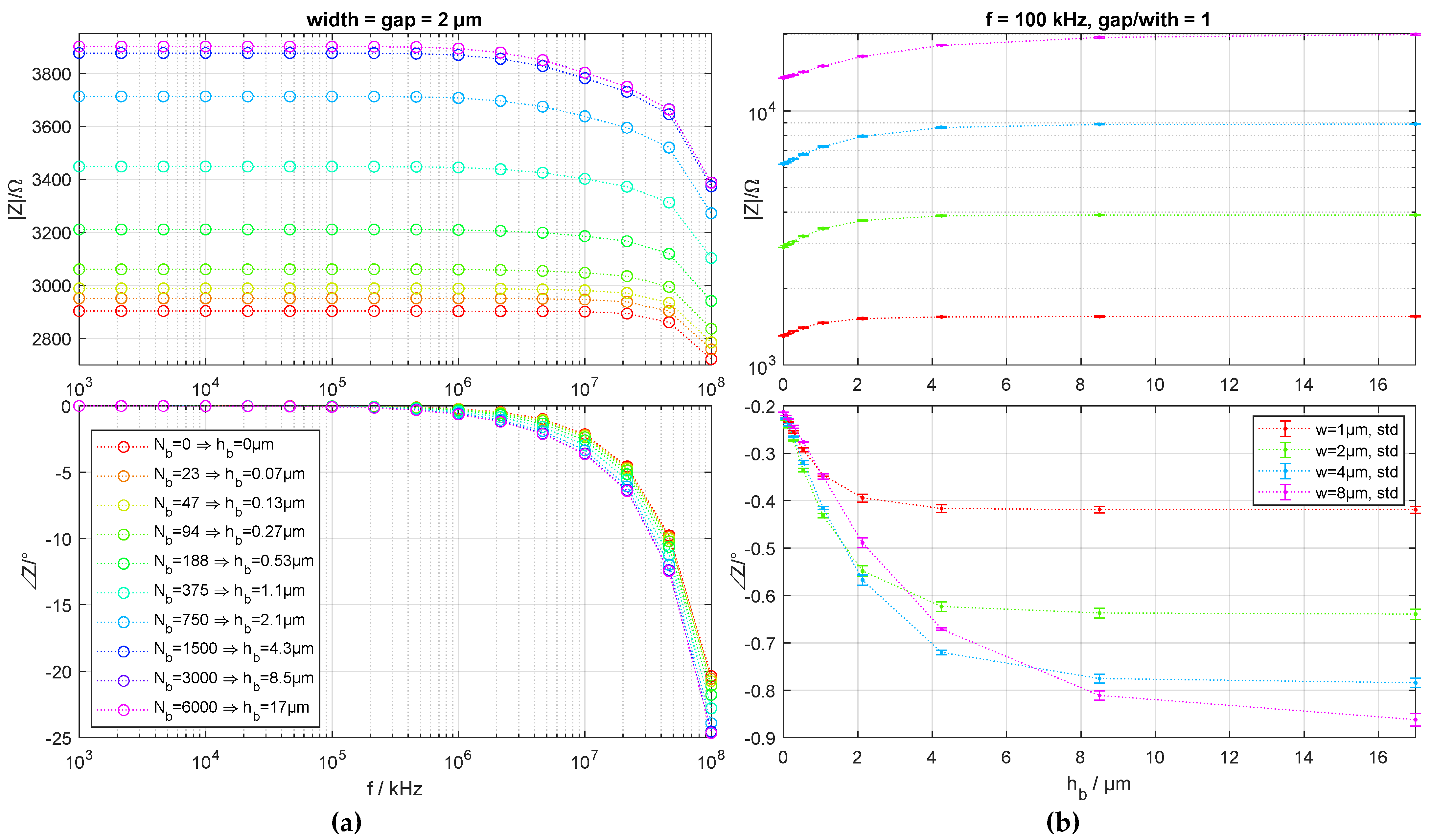
Figure 9a shows the mean values of the impedance spectra for the electrode size $w$ = $g$ = 2 µm. As expected, a typical low-pass behavior is shown (as indicated in Figure 1b). Amounts and phases decrease with increasing frequency. The higher the biofilm, the higher the capacitive component and the higher the decrease in magnitude and phase. At $h_b$ = 0 (red line), only the capacitance of the electrodes has a frequency-dependent effect, and the magnitude only changes significantly from approx. 50 MHz, whereas at $h_b$ = 17 µm, the influence of the biofilm can clearly be seen from approx. 1 MHz. The change in the impedance value of $h_b$ is highest at low frequencies. Here, the capacitances of the bacterial membranes act almost like insulators and the displacement of the measurement medium by the bacteria has a greater effect on the value than at high frequencies, where the resistance of the bacteria decreases (Figure 10). In contrast, the phase difference as a function of $h_b$ is higher at high frequencies, as the current flow through the bacteria and thus the phase shift of the current increases as the frequency increases.

Figure 9b shows the dependence of impedance magnitude and phase on $h_b$ for the individual electrode sizes at a typical measurement frequency of 100 kHz. The higher the distance between the electrodes, the higher the resistance. As a first approximation, the impedance value doubles with the electrode spacing. The resistance also increases as the biofilm grows, as the biofilm has a lower conductivity than the medium. As the number of bacteria increases, the capacity increases and consequently the phase shift as well. It can already be seen in this raw data that the differences between $h_b$ = 0 and $h_b$ = 17 µm are highest at large electrode spacing—both in terms of magnitude and phase.

The standard deviation of the impedances between the three geometrically different biofilm models is always less than 1%. This means that the influence of the orientation of the individual bacteria is small.

Another result is that at $h_b$ = 0, the cut-off frequency for all combinations of electrode width and distance is constant at 270 MHz. This high value results from the high conductivity of the medium. The independence of the electrode size results from the fact that the cut-off frequency of a simple first-order low-pass filter is determined by $f_g$ = $1/\left(2\pi fRC\right)$, and the $RC$ factor (resistance and capacitance between the electrodes) remains constant when the electrode size changes. If the distance between the electrodes increases, $R$ increases and $C$ decreases. Only a change in the conductivity or permittivity of the medium would have an influence on the cut-off frequency. In reality, however, the measurement would be limited even at much lower frequencies by the impedances of the leads and the front end.

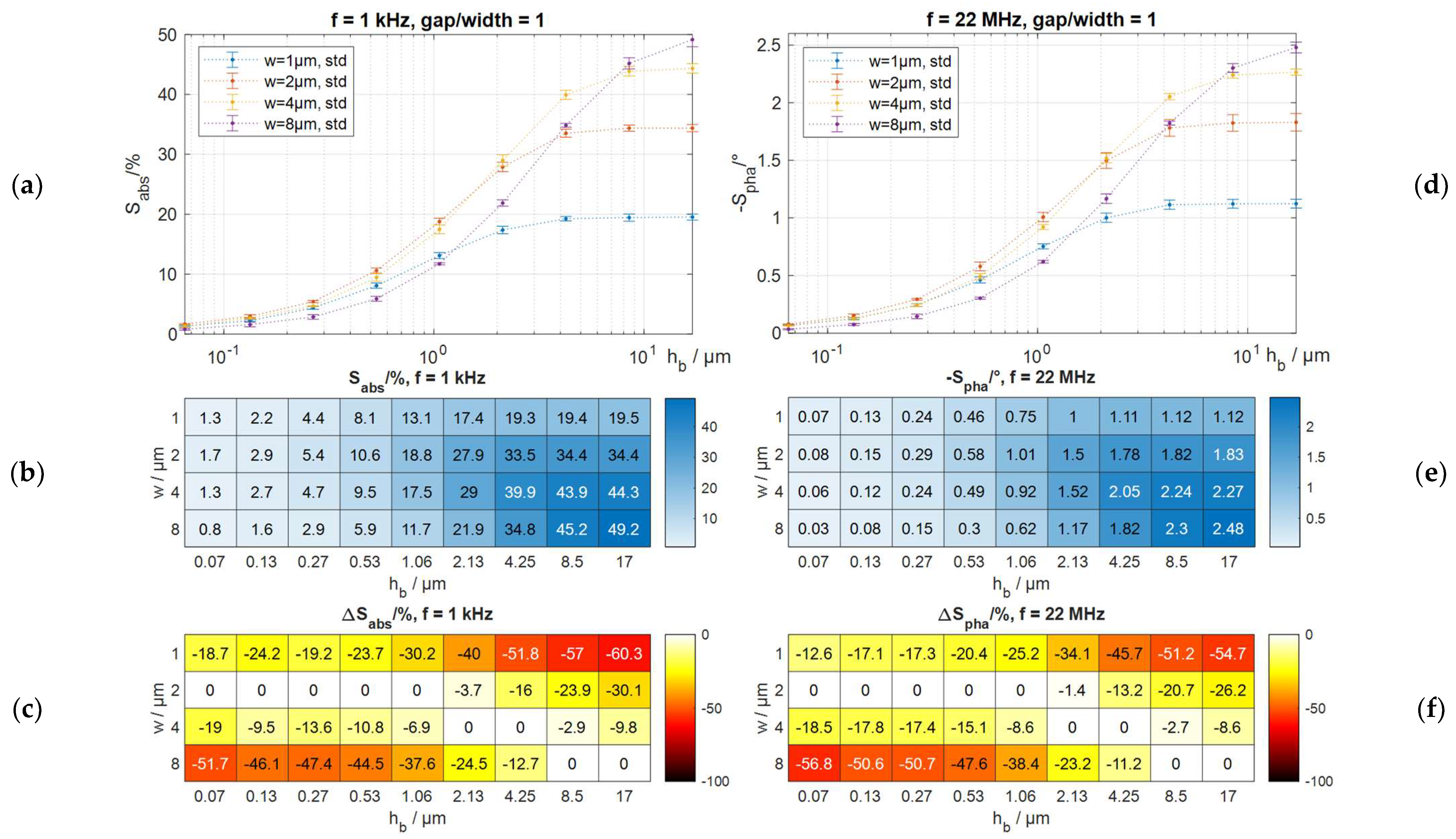
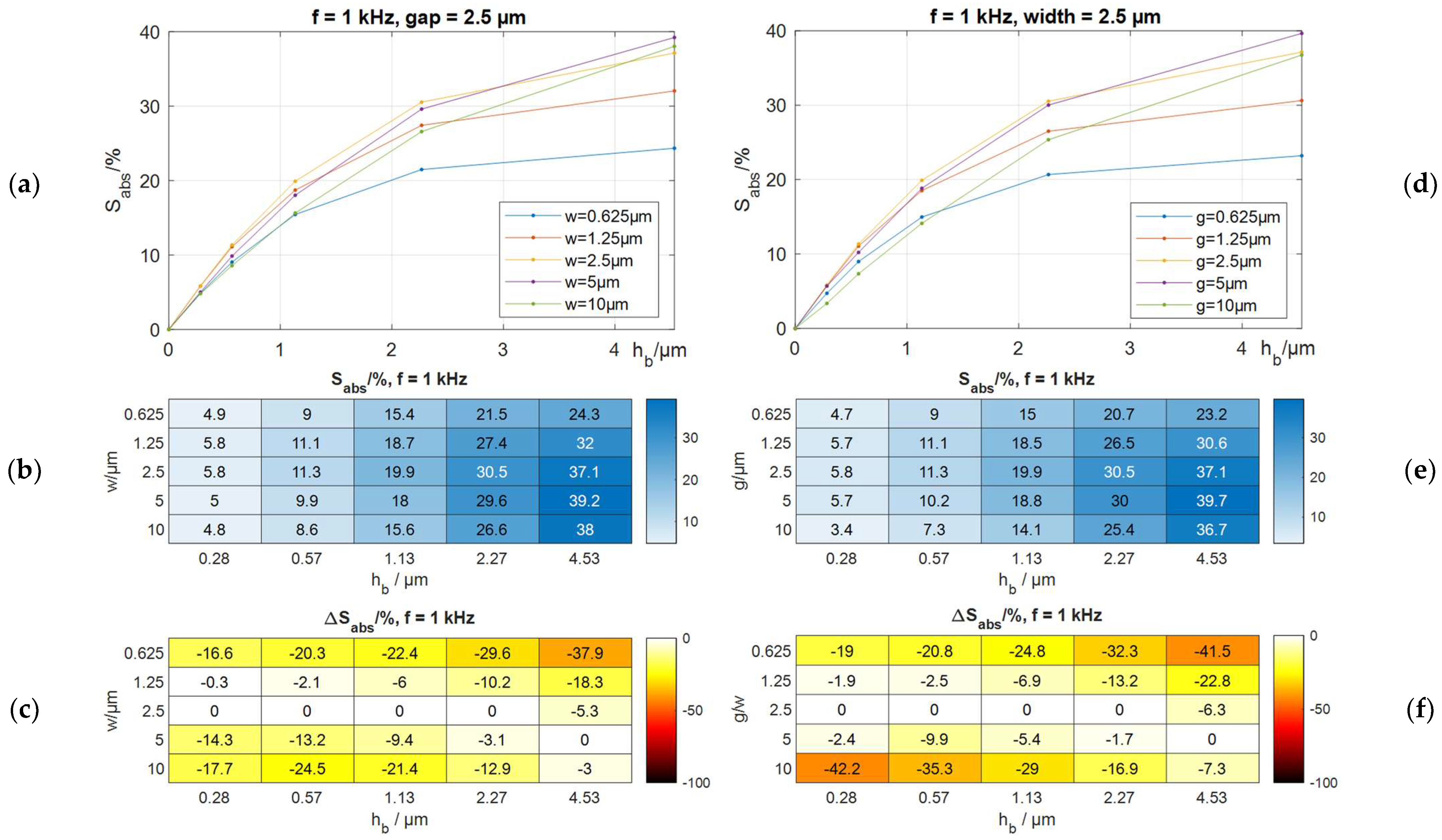
3.2. Optimum Electrode Widths and Gaps

In order to determine at which electrode widths w and gaps g the sensitivities $S_{abs}$ and $S_{pha}$ (see Formulas (1) and (2)) become maximum, a simulation was carried out with 4 electrode geometries, 10 growth stages of the biofilm, and 16 frequencies. To evaluate the standard deviation, this simulation was carried out three times with different biofilms. A data set with 4 × 10 × 16 = 640 impedances is, therefore, available in triplicate for the evaluation. From this, mean values and standard deviations were calculated.

The results for the impedance magnitudes are shown for the lowest frequency of 1 kHz (Figure 11), as $S_{abs}$ is highest in this frequency range. The phases are shown for 22 MHz, as the phase differences are higher at high frequencies. As the values at low $h_b$ are difficult to recognize in the upper graph, $S_{abs}$ and $S_{pha}$ are shown in the middle as a heat map.

In order to highlight which electrode sizes are most sensitive at which biofilm heights, the sensitivities were normalized again to the respective maximum for each $h_b$ to calculate the differences $\mathsf{\Delta }{S}_{abs}$ and $\mathsf{\Delta }{S}_{pha}$. These are shown as a heat map in Figure 11c,f.

$$\mathsf{\Delta }{S}_{abs}\left(w\right)=\frac{S_{abs}\left(w\right)}{\max \left(S_{abs}\left(w\right)\right)}-1,$$

(3)

$$\mathsf{\Delta }{S}_{pha}\left(w\right)=\frac{S_{pha}\left(w\right)}{\max \left(S_{pha}\left(w\right)\right)}-1$$

(4)

The highest sensitivities for all electrode sizes are found for the largest biofilm height, as the change in impedance is highest here compared to $Z_0$ (impedance without biofilm). For the electrode size $w$ = 8 µm, the sensitivity is highest with $S_{abs}$ = 49%. In comparison, the electrode with $w$ = 1 µm has a 60% lower sensitivity. At the beginning of biofilm growth (low $h_b$), the electrode with $w$ = 2 µm is the most sensitive. Although the maximum sensitivity is only 1.7% at $h_b$ = 0.07 µm (corresponds to $N_b$ = 23), this is still the possible maximum. In comparison, the sensitivity of the largest electrode is 52% lower here. The behavior of the phases is equivalent to that of the magnitudes.

The electrode size $w$ = 2 µm consistently has the highest sensitivity up to a biofilm height of 1 µm. As can be seen in Figure 5, these are the heights at which most bacteria are still in direct contact with the electrode surface. At bigger heights from $h_b$ = 2 µm, most of the bacteria are already on top of each other. In this area, the current density distribution at $w$ = 2 µm is no longer optimal and the electrode with $w$ = 4 µm has a better sensitivity (see also Figure 2). The electrode with $w$ = 8 µm only has the highest sensitivity at $h_b$ = 8.5 µm. The electrode with $w$ = 1 µm has an unsuitable distribution of the current density overall so that it has a comparatively poor sensitivity at all $h_b$.

The standard deviation of the sensitivities is so small that the above statements can be made with certainty. The electrode area is, therefore, already so large that the random alignment of the individual bacteria has no significant influence.

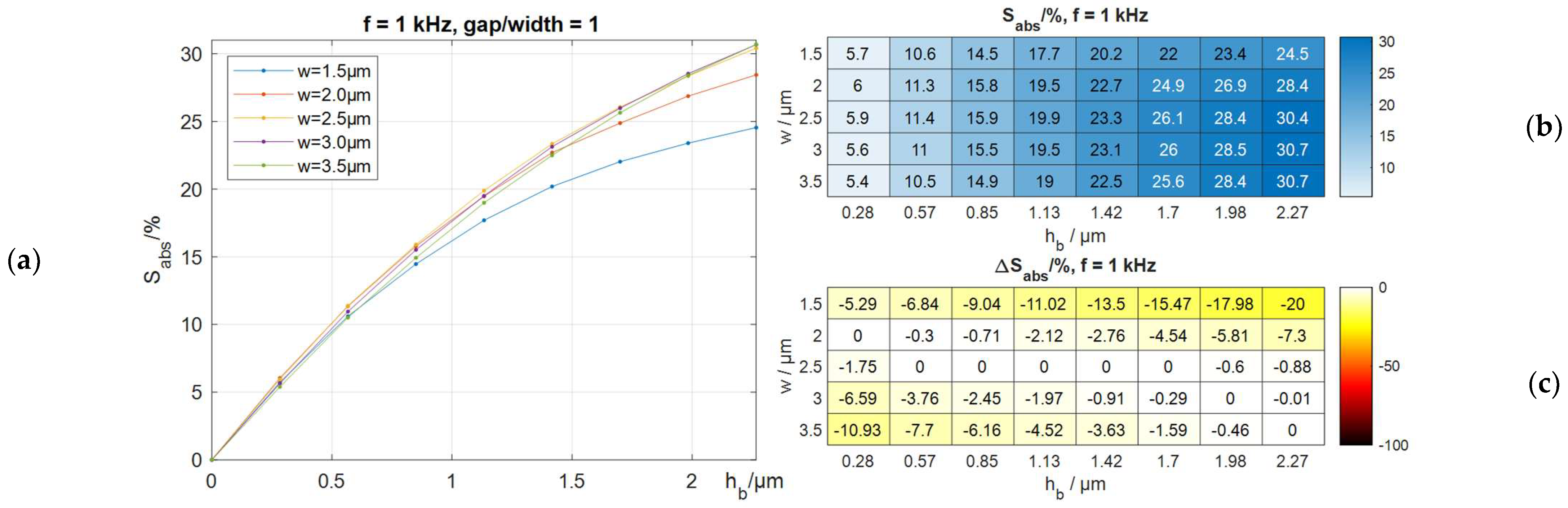
As the difference between the above electrode sizes is very large, the simulation was repeated with a finer resolution to determine at which exact size the sensitivity for thin biofilms becomes maximum. Again, the electrode spacing is equal to the electrode width. The result is shown in Figure 12. It can be seen that an electrode width of 2.5 µm is slightly more sensitive than a 2 µm electrode. The differences are very small, and at the lowest $h_b$, the 2 µm electrode is even slightly, 1.8%, more sensitive.

If the priority is to measure low biofilm heights as sensitively as possible, the decision for an electrode size of $w$ = $g$ = 2.5 µm would be made for the given biofilm. If the priority is to measure thicker biofilms, the corresponding larger geometries should be selected. If the focus is on measuring both thin and thick biofilms, a multi-channel setup with several corresponding electrodes can be selected.

3.3. Optimum Ratio of Electrode Width and Gap

In the results shown in the previous section, the values for electrode width $w$ and gap $g$ were equal. In other simulations, it has been investigated how the sensitivity changes when $w$ and $g$ assume different values. In one simulation run, the width was kept constant at $w$ = 2.5 µm and the distance $g$ was varied. And in another simulation run, the distance was kept constant at $g$ = 2.5 µm and $w$ was varied. As can be seen in Figure 13, the results are almost identical. At a low biofilm height $h_b$, the ratio $g/w$ = 1 is optimal. 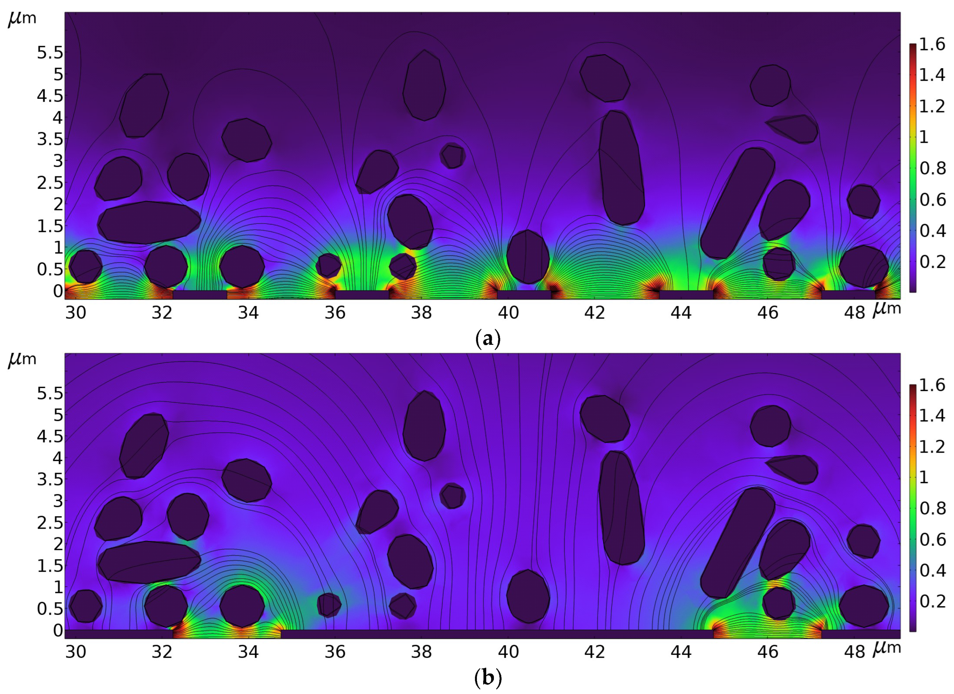From h_b = 4.5 µm, the electrodes with higher width or higher distance are more sensitive. The current densities in Figure 14 illustrate the difference between two electrodes with the same distance but different widths. At a higher distance, the proportion of the current flowing through higher areas is higher. As a result, larger electrodes are more sensitive at large $h_b$.

4. Conclusions

The specific result of this study is that an IDE with a width of 2.5 µm and a gap of 2.5 µm is the most sensitive for measuring initial biofilm growth. This confirms the rule of thumb that the electrode size should correspond to the size of the structure to be measured. Electrodes with larger gaps/widths are only more sensitive if the biofilm height is significantly bigger than 2 µm. This result applies to the bacterial model used based on E. coli in the specific environment.

The general result of this study is more comprehensive. Since both the algorithm for biofilm generation and the scripts for generating the FEM model are parameterized, the calculations can be carried out for other bacteria in other media with little effort. With the methodology presented, the most sensitive electrodes can be easily chosen for a wide range of biofilms and environments. The method is not only important for the most sensitive measurement of biofilm growth but also for the characterization of biofilms. The sensitivity of biofilm measurement is always maximized if the largest possible proportion of the current flows through the biofilm. In this case, the properties of the biofilm (cell membrane, protoplasm) can also be measured as best as possible.

5. Outlook

Up to now, biofilm models have been generated with bacteria of a constant size. It therefore makes sense to modify the generation algorithm so that an arbitrary distribution of bacteria of different sizes can be generated within a biofilm. It would also be possible to assign different electrical properties to individual groups of bacteria for the FEM simulation. In this way, electrode sizes can also be optimized for biofilms with multiple species.

In many applications, the conductivity of the medium is not constant over time, as there is no fluid flow through the measuring chamber. To take this case into account, different conductivities of the medium could be used in the model for the individual growth stages of the biofilm.

Another promising application of the presented model is the development of electrical equivalent circuit diagrams of biofilms. When measuring the impedance of biofilms, the measurement result is usually fitted to models. These models or equivalent circuit diagrams often do not match the electrical parameters of the biofilm, resulting in a significant deviation between measurement and fit. The algorithms presented in this study can be used to generate and measure any biofilm. The fact that the simulated electrical properties of the biofilm are already precisely known makes it much easier to develop a suitable impedance model.

The results of the simulation are plausible, but they still need to be compared with real measurements. For this purpose, electrodes of different sizes will be designed and manufactured on the basis of the simulation results. These will then be used in real biofilm measurements to verify the results of the simulations.