Abstract
In this paper, we investigated rates of admission to hospitals (or other health facilities) due to respiratory diseases in a United States working population and their dependence on a number of demographic and health insurance-related factors. We employed neural network (NN) modelling methodology, including a combined actuarial neural network (CANN) approach, and model admission numbers by embedding Poisson and negative binomial count regression models. The aim is to explore the gains in predictive power obtained with the use of NN-based models, when compared to commonly used count regression models, in the context of a large real data set in the area of healthcare insurance. We used nagging predictors, averaging over random calibrations of the NN-based models, to provide more accurate predictions based on a single run, and also employed a k-fold validation process to obtain reliable comparisons between different models. Bias regularisation methods were also developed, aiming at addressing bias issues that are common when fitting NN models. The results demonstrate that NN-based models, with a negative binomial distributional assumption, provide improved predictive performance. This can be important in real data applications, where accurate prediction can drive both personalised and policy-level interventions.
1. Introduction
Chronic respiratory diseases (CRDs) remain one of the main causes of morbidity and mortality worldwide. The World Health Organization (WHO) reports that hundreds of millions of people worldwide suffer from preventable CRDs, and these diseases cause around four million deaths each year (Bousquet et al. 2007). Asthma, chronic obstructive pulmonary disease (COPD), and occupational lung disease are some of the major diseases classified under preventable CRDs. As per the WHO, 262 million people have asthma globally, and over 3 million people die each year from COPD, which accounts for nearly 6% of deaths around the world (WHO 2022b). The recent COVID-19 pandemic has once again put CRDs in the limelight due to the notion that people with pre-existing respiratory conditions are at a high risk for COVID-related health complications and death. Although some studies, such as Aveyard et al. (2021), support this, owing to the lack of data, the extent of higher risks from COVID for individuals with CRDs is still unclear (WHO 2022a). Most CRDs are preventable through early detection and intervention, which require precise identification and understanding of the key risk factors and their association with the incidence and prevalence of these diseases. Previous studies, such as Doney et al. (2014) and CDC (2012), have explored the prevalence of COPD among the US population, whereas Blanc et al. (2019) focused on the relationship between workplace exposure and respiratory diseases.
Ever since generalised linear models (GLMs) were introduced by Nelder and Wedderburn (1972), they have been at the forefront of predictive modelling in all areas of research. Details regarding numerous applications of GLMs for tackling insurance-related actuarial problems in both life and non-life sectors are described in Haberman and Renshaw (1996), De Jong and Heller (2008), Frees (2009), and Ohlsson and Johansson (2010). The advancement in computational capabilities and the development of software, such as Bayesian inference using Gibbs sampling (BUGS), have further facilitated the Bayesian implementation of GLMs. For instance, in an insurance-related context of morbidity studies, Ozkok et al. (2014) adapted Bayesian methodologies for modelling claim diagnosis rates of critical illness; more recently, Arık et al. (2021) conducted a population study for assessing the socioeconomic disparities in cancer incidence and mortality in England.
Improvements in the ease of access to fast computing over the last few decades have paved the way for the extensive adaptation of machine learning approaches in many research and practice areas. The same pattern has been observed in the insurance field, particularly in recent years. There is an increasing trend in applying machine learning approaches for addressing various insurance-specific problems. Blier-Wong et al. (2020) provided a detailed description of recent adaptions of different machine learning approaches in the actuarial field, particularly for pricing and reserving. Ferrario et al. (2020) detailed the adaptation of neural network regression models for modelling claim rates using the French motor third-party liability (MTPL) insurance data set. The approach facilitates the embedding of traditional regression models for count data into a neural network framework using a class of feed-forward neural network (FFNN) models. For the rest of the paper, we refer to the FFNN and neural network (NN) indifferently. The approach was further extended by Schelldorfer and Wuthrich (2019) to develop the combined actuarial neural network (CANN) approach (see Section 3.3 for details), which showed superior performance in comparison to the previous NN model. Tzougas and Li (2021) added to the approach by developing both NN and CANN models under a negative binomial distributional assumption.
In this work, we developed an ensemble of statistical predictive models that can accurately predict admission rates to hospitals (or other health facilities) related to respiratory diseases in a US population. In what follows, we outline the main contributions of the paper.
- First, we investigated the efficiency of the Poisson and negative binomial CANN models for predicting admission rates related to respiratory diseases in a United States (US) working population. In particular, we began by considering Poisson NN models, including a CANN model, and developed modifications based on early stopping and dropout techniques, which improve their performances. Subsequently, motivated by the suitability of the negative binomial distribution when data are over-dispersed, we also developed negative binomial NNs and compared their predictive performances to those of the Poisson models. NN-based models were trained by minimising the corresponding deviance loss functions and compared using the testing data loss. Models under the negative binomial distributional assumption led to superior forecasting performances. The same result was obtained when we eventually compared the Poisson CANN to the negative binomial CANN. Furthermore, it is worth noting that while machine learning approaches and CANN models, under both Poisson and negative binomial distributional assumptions, have been explored for data-driven applications in the field of non-life insurance, to the best of our knowledge, this is the first paper that considered employing such methods for morbidity modelling in an insurance context.
- Second, we considered the bias-regularised version of the negative binomial NN and CANN models by modifying the intercept of their output layers following the approach of Wüthrich (2020). Additionally, we also addressed bias issues on a population level by extracting the last hidden layer of the NN and CANN models, fitting the corresponding negative binomial regression models and, therefore, controlling the portfolio bias by adjusting the intercept.
- Third, following the setup of Richman and Wüthrich (2020), we determined a nagging predictor in the case of the negative binomial NN and CANN models for taking advantage of the randomness of neural network calibrations to provide more stable predictions than those under a single neural network run.
- Finally, for providing reliable comparisons between the performance of the regression, NN, and CANN models under the negative binomial assumption, k-fold validation was carried out to allow us to evaluate the model’s predictive ability when different data configurations were considered for training and prediction purposes.
The rest of this article is as follows: in the next section, we present a description of the data used in this paper and we provide details of the exploratory analysis that was carried out for summarising the main data characteristics. A number of data considerations, prior to undertaking any modelling approaches, are also discussed. In Section 3, we provide a detailed description of the regression, NN, and CANN models that were used for modelling the admission rates. In Section 4, we present hyperparameter tuning and determine the approach that was followed for fitting the network-based models. Various model improvement approaches, such as regularisation, dropout, and early stopping, were adopted for the network models, and are presented in Section 5. In Section 6, a comparison of the predictive performance of the competing models under Poisson and negative binomial distributional assumptions is presented, along with bias-regularised versions and a nagging predictor for the negative binomial NN and CANN models. Furthermore, an evaluation of the performance of the negative binomial regression, NN, and CANN models via k-fold validation is carried out in Section 7. Finally, concluding remarks are provided in Section 8.
2. Data
The admission data for respiratory diseases were constructed using the Commercial Claims and Encounters Database of Merative MarketScan Research Databases provided by Merative (previously called IBM Watson Health). The data set contains individual-level information regarding admissions to hospitals and other health facilities, along with the claims and encounter data over time, linked with patient information and service provider details. For categorizing the admissions with respect to the primary cause of admission, the International Statistical Classification of Diseases and Related Health Problems 10th Revision—Clinical Modification (ICD-10-CM) groupings were used (see Table A1). The data set was constructed by combining the admission information and the enrollment details for the year 2016, and the details of the different variables in the data set constructed are given in Table 1.

Table 1.
Description of variables in the admission data set.
The ENROLID is a unique identifier assigned to each individual. The EMPREL variable specifies the individual’s relationship to the primary beneficiary/employee. The different plan types defined by the PLANTYP variable vary in terms of their characteristics, such as incentives for using specific service providers, deductibles, copay, etc. …For more details regarding the different plan types, see Table A3. The geographical variable EGEOLOC gives more granular information regarding the primary beneficiary’s residence location than the REGION variable. The UR variable was created using the Metropolitan Statistical Area (MSA) variable by assigning value 1 (rural) if the primary beneficiary resides in a non-MSA or rural area and value 2 (urban) if the primary beneficiary resides in MSAs. The EECLASS and EESTATU variables give information regarding the employment of the individual. The DATATYP indicates whether the individual’s health plan operates as a fee-for-service plan or a capitation plan. The difference is that the fee-for-service works on a reimbursement basis while the encounter record arises from fully or partially capitated managed care plans. The prepaid capitation amount paid by the employer or the health plan to the service provider could either be on an individual basis or a bulk basis. The details of the primary beneficiary are assigned to the spouse and other dependents as well. Prior to undertaking any modelling, several data considerations and feature preprocessing were undertaken, details of which are described in the following subsections.
2.1. Data Description
The admissions records of an individual within two days were treated as a single admission. Data variables with a high proportion of missing data (e.g., INDSTRY) were excluded. For the other variables, only complete cases were considered as the proportion of missingness was less than 2%. Variables, such as HLTHPLAN, DATATYP, and REGION were excluded due to the high level of relationship with other variables. The HLTHPLAN variable had a high level of association with EECLASS and EESTATU variables. The employment-related information, particularly the employment classification, was only available if the data came from the employer (HLTHPLAN = 0). Hence, for all the individuals whose data came from health plans, the EECLASS was unknown (category 9). The association between PLANTYP and DATATYP arises since the value of the DATATYP variable is 2 (Encounter) only for individuals under the Health Maintenance Organization plan (PLANTYP = 4) and Capitated (Cap) or Partially Capitated (PartCap) Point-of-Service plan (PLANTYP = 7). The EGEOLOC variable was chosen over the REGION variable as it gives more granular information regarding an individual’s location of residence.
After the above-mentioned data considerations, the data for the age range 30–65 comprises 2,050,100 records, with 1,902,840 unique individuals and 100,212 admissions due to various diseases. The age range selection of 30 to 65 was used as the focus is on the working population and 30–65 seemed to be a reasonable choice for working age. The circumstances of some individuals changed over the year and, hence, their risk characteristics changed as well. Multiple records with different risk characteristics exist for those individuals for the corresponding period. This results in having more records than the number of unique individuals. Although multiple records might exist for some individuals, the sum of the exposure over different records for any given individual is less than or equal to one year. The distribution of admissions over the different ICD chapters is shown in Figure 1.
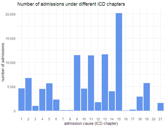
Figure 1.
Distribution of admissions over different ICD chapters (details about chapters in Table A1).
Among these 100,212 admissions, 4525 were related to respiratory diseases (ICD chapter 10), and some individuals had more than one admission. The most prominent cause of admission was pregnancy and childbirth (ICD chapter 15), followed by diseases related to the musculoskeletal system and connective tissue (ICD chapter 13), diseases of the circulatory system (ICD chapter 9), and diseases of the digestive system (ICD chapter 11). Admission frequencies due to respiratory diseases are given in Table 2, and the age-wise crude rates of admission for different categories of the variables such as SEX, UR, and EECLASS are shown in Figure 2.
Table 2.
Frequency of number of admissions related to respiratory diseases for individuals under the age range 30–65.
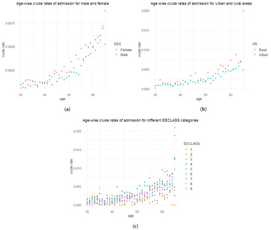
Figure 2.
Age-wise crude rates of admission due to respiratory diseases: (a) male, female; (b) urban and rural areas; (c) categories of EECLASS.
As unusually high numbers of individual admissions are often the result of common healthcare data practices, the ceiling for the number of admissions for an individual was set as five in the current analysis. Hence, the final data set involves 4513 admissions related to respiratory diseases. In order to determine whether to use EXPOSURE as an offset variable, an exploratory analysis similar to the one mentioned in Ferrario et al. (2020) was carried out. The records were categorised using an additional ‘Exposure group’ variable defined by with , which indicated that a significant proportion of the 2,050,100 records belonged to group with exposure . A group-wise empirical frequency was also calculated by where represent the number of admissions for the ith record (see Table 3).
Table 3.
Relative number of records and empirical frequency for each exposure group.
Even though the empirical frequencies of exposure groups give no evidence of suspecting the non-linearity of exposure, to identify any potential relationship between the exposure and other features, the distribution of exposure over other variables was also investigated (see Figure 3).
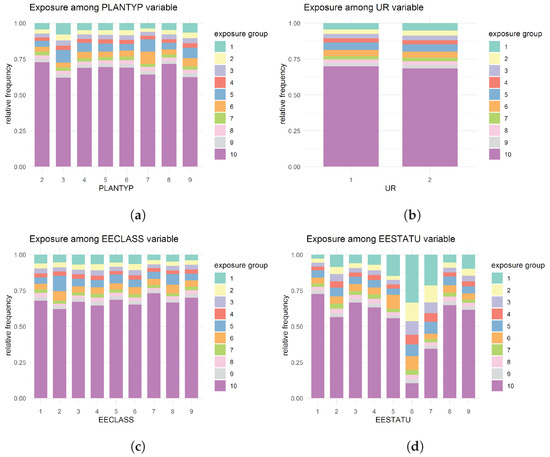
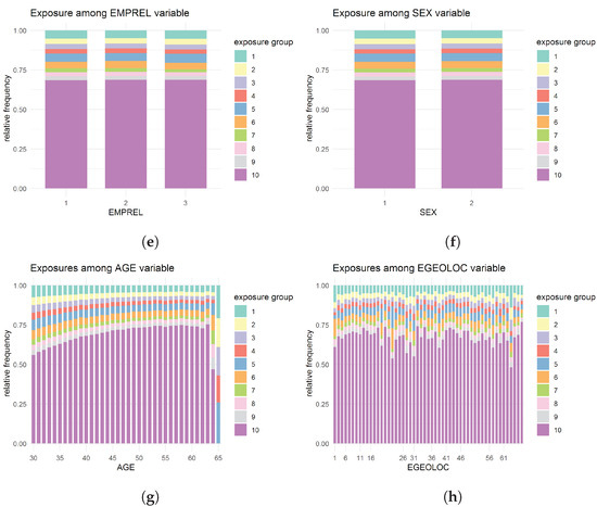
Figure 3.
Distribution of exposure over different variables: (a) over PLANTYP variable; (b) over UR variable; (c) over EECLASS variable; (d) over EESTATU variable; (e) over EMPREL variable; (f) over SEX variable; (g) over AGE variable; (h) over EGEOLOC variable.
Although the analysis indicates a slight variation in the exposure composition over different levels of some variables, the evidence is not strong enough to consider alternative treatments of the exposure variable. For instance, for the EESTATU variable, unlike the other categories, for category six (Comprehensive Omnibus Budget Reconciliation Act (COBRA) continues), the exposure seems to be evenly distributed. COBRA allows employees and their dependents to continue with a health plan provided by an employer for a particular period even after the cessation of their employment with that employer. Individuals with EESTATU six (COBRA) may have reached the end of that specified period sometime during the year of the study (2016). Although this could be a case of right censoring, we lack sufficient information to confirm this. Hence, it was decided to proceed with treating exposure as an offset variable.
2.2. Data Pre-Processing
The full data set was randomly split into a learning set and a testing set . The learning set and testing set were created using a 90:10 split, comprising 1,845,090 and 205,010 records, respectively. All models were fitted using the learning data set, and the performances of the models were evaluated on the testing set under the assumption that the underlying modelling assumptions held for both sets of data.
As discussed by Ferrario et al. (2020), the proper working of the gradient descent methods (GDMs) used for neural network model fitting required the different feature components to be on an identical scale. In order to adjust the scaling, for the continuous and binary variables, such as AGE, SEX, and UR, a min–max scaler was adopted, which transformed the variable to a scale of using the formula:
where and represent the minimum and maximum values of variable . For the binary variables SEX and UR, the values would have been replaced by either −1 or 1. For all remaining categorical variables, since they were nominal in nature, a dummy encoding was used. Under dummy encoding, a categorical variable with l levels was represented using a dimensional feature vector, with a reference category and value 1 being used to identify the actual level for a data record (see Equation (2)). An alternative option was to use one-hot encoding, which would have resulted in an dimensional feature vector without a reference level (Equation (3)). For a categorical variable , with l categories , treating as the reference level, dummy encoding is given by
whereas one-hot encoding would take the form
As both approaches increase the dimension of the feature space, for neural network models, data embedding was implemented using an embedding layer, which facilitated a lower dimensional representation of the categorical variables. The embedding layer approach was proposed by Bengio et al. (2000) and was adopted in an insurance context by Richman and Wüthrich (2021). The embedding layer maps a categorical variable with l levels to a low dimensional real-valued vector of dimension v ( (i.e., ). The value of v, which is treated as a hyperparameter, needs to be decided, taking into consideration that it impacts the complexity of the model. In the current context, we chose for creating the embedding layers for categorical variables (see Figure 4).
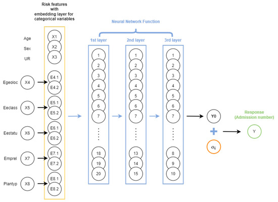
Figure 4.
A sample representation of a feed-forward neural network with embedding layers and three hidden layers with 20,15,10 neurons in each layer.
3. Models
3.1. Regression Models
We first consider a Poisson GLM and a negative binomial regression model, for modelling count data (e.g., Frees 2009; Hardin et al. 2007). For the Poisson GLM, we assume that for , n being the number of records in the learning data set , admission numbers, , follow a Poisson distribution with
where the mean depends on the policyholder’s characteristics through , and the exposure . By choosing the logarithmic link function, which is, in fact, with the canonical link function for the Poisson GLM, we have a predictor of the form
where is the feature space with giving the feature information. is the offset term, and is the unknown vector of coefficients to be estimated. The represent the inner products of vectors and and are equivalent to ; both notations are used interchangeably in this paper.
Similarly, for the negative binomial regression model, admission numbers, , , are assumed to follow a negative binomial distribution with a dispersion parameter :
with
For a logarithmic link function, the predictor has the form
3.2. Neural Network Model
In what follows, we consider the basic feed-forward neural network (FFNN) model. Generally, a FFNN comprises an input layer, one or more hidden layers, and an output layer. The feature space makes up the input layer, and each of the hidden layers comprises a set number of neurons. The output from a given hidden layer acts as the input for the next layer. The output from a neuron depends on the linear combination of the output from the previous layer and the choice of activation function assigned to the layer that it is part of (see Section 4 for more details on activation function). The number of hidden layers is treated as a hyperparameter and is also referred to as the depth of the network. The last layer of the architecture, which is connected to the last hidden layer, is the output layer. In a neural network architecture, each layer is a function of the previous layer (see LeCun et al. (2015) and Ferrario et al. (2020) for more details). The mth hidden layer with dimension can be defined as
where the neurons are given by
with being the activation function and the network parameters. In addition to the first intercept component, depends on . For , with q being the dimension of the feature space , the network parameter will have dimension r where
A diagrammatic representation of a feed-forward neural network with an embedding layer and three hidden layers with 20,15,10 neurons in each layer, are shown in Figure 4.
Under a neural network regression model, the predictors and of the traditional Poisson and negative binomial regression models are replaced by the neural network predictors and . To illustrate the structure of the network-based model, we will refer to the models under the Poisson distributional assumption. For an FFNN model with depth d under the Poisson assumption, the predictor is of the form
for , where are the weights that map the neurons of the last hidden layer to the output layer .
3.3. CANN
As mentioned earlier, the CANN model has an additional regression function nested into the model predictor using a skip connection. Under the Poisson distributional assumption, the model predictor of the CANN model with depth has the form
with and parameter vector . The vector represents the parameters associated with the skip connection. The three terms on the right-hand side of Equation (13) represent the offset, regression function/skip connection, and the network function, respectively. A schematic representation of a sample CANN model with three hidden layers and 20,15,10 neurons in each layer is shown in Figure 5.
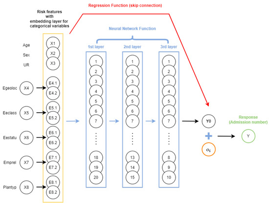
Figure 5.
An illustration of a sample CANN model with three hidden layers and 20,15,10 neurons in each layer.
As shown in Figure 5, feature space is directly linked to the output layer. Different variants of CANN exist depending on whether the weights in the regression part are updated or not whilst training the model (Schelldorfer and Wuthrich 2019). Owing to the ease of implementation and following the literature, we focus on the variant in which the weights of the regression component are kept fixed as the iterated weighted least squares (IWLS) estimate from the regression model. This particular variant of the CANN can be implemented by replacing the offset term in Equation (13) with
The approach can be enacted indifferently under both Poisson and negative binomial distribution assumptions by adjusting the likelihood function under each model and altering the sample code given in Listing A1. For the models under the Poisson distribution assumption, with being the response variable and the mean for regression, for FFNN and for CANN), the log-likelihood is of the form
Likewise, for the negative binomial models, under the NB2 parameterisation (Hardin et al. 2007), the log-likelihood is given by
The details of the fitting of the different models discussed so far are discussed in detail in the next section.
4. Model Fitting
The different data considerations and exploratory analysis described in the earlier sections, as well as the development of models described in the previous section, were carried out using the programming language R using RStudio IDE (R Core Team 2021; RStudio Team 2021). The Poisson and negative binomial regression models were fitted using the glm() function in the stats package and the gamlss() function in the gamlss package. The glm() uses the IWLS method whereas gamlss() function uses the Rigby and Stasinopoulos (RS) algorithm, for estimating the model coefficients (R Core Team 2021; Rigby and Stasinopoulos 2005). The two main packages utilised for developing the neural-network-based models are keras and TensorFlow packages, details of which can be found in the respective manuals Allaire and Chollet (2021) and Allaire and Tang (2021). The important snippets of code developed for implementing NN and CANN models, as well as the different model improvement approaches, are given in the Appendix A.
4.1. Hyperparameters
The development of the network-based models was carried out in different stages. The first step of constructing the models involves determining the hyperparameters, such as the number of hidden layers, choice of activation function, and the gradient descent method (GDM) used for model training. In terms of the aspects mentioned above, following earlier work by Ferrario et al. (2020) in a similar context, the following assumptions were made:
- Number of hidden layers: the number of hidden layers was kept at three.
- Activation function: for hidden layers, the hyperbolic tangent function, , was used. Any alternate non-linear activation function would work. The motivation behind a non-linear activation function is that a non-linear activation function allows for a non-linear model space, reducing the number of nodes needed and allowing the network to automatically capture the interaction effect of different features. For the output layer, an exponential function was used, which is the inverse of the link function () and, therefore, is in line with the underlying distributional assumption.
- Gradient descent method: the neural network training utilises a gradient descent optimisation algorithm for estimating the model weights. Ferrario et al. (2020) compared different GDMs in terms of performance and identified the Nesterov-accelerated adaptive moment estimation (Nadam) method as performing better compared to other similar methods. Hence, we also adapted the Nadam as the choice of GDM. An overview of the different GDMs is given in Ruder (2016), and additional details regarding the ‘Nadam’ method could be found in Dozat (2016).
- Validation set: the training of neural network models requires further splitting the learning set into a training set, , and a validation data set, . The validation data set is used as the evaluation set during the iterative process for estimating the model weights. In other words, tracks possible overfitting of the model to . For the network-based models discussed here, and an 80:20 split was used for the training and validation data sets. Once the training is complete, the final performance of the fitted model is assessed using the testing set.
- Loss function: the loss function is the objective function that the GDM algorithm minimises in order to estimate the model weights (Goodfellow et al. 2016). Numerous options exist in terms of the choice of the loss function. For instance, mean squared error (MSE), mean absolute error (MAE), and deviance loss are some of the popular choices of loss functions used in a regression problem. For our context, we adapted deviance loss as the loss function. The motivation behind the particular choice is that minimising the deviance loss is equivalent to maximising the corresponding log-likelihood function, which gives the MLE. The deviance loss is defined as the difference between the log-likelihood of the saturated or full model and the fitted model, and for a data set the Poisson deviance loss is given bywhere denotes the fitted mean and the observed number of admissions for . Similarly, for models under the negative binomial distributional assumption, the deviance loss function has the form:
The GDM estimates the model weights by minimising the deviance loss for the learning set, and the performance of the thus fitted models can be compared using the deviance loss for the testing set. As described earlier, the GDM updates model weights with an improved choice in an iterative manner. The iterative updation of model weights under the GDM could be represented as
where indicates the algorithmic step, and gives the learning rate and are the mini-batches or batches (see next section for more details on batches). The learning rate determines the size of each step and influences the speed of movement towards the optimal model weights. Since the primary focus of this work is the predictive modelling of admission rates, more details relating to the functionalities of the neural network model training are not discussed further (see, e.g., Russell 2010; Goodfellow et al. 2016).
4.2. Batch Size and Epochs
In addition to the model choices discussed above, the other main model attributes that need to be determined are the number of neurons in each layer, batch size, and epochs. Due to the computational burden of considering a large data set at once, during the training of a neural network, the data in the training set are considered in smaller batches created randomly, having approximately the same size . The batch size b refers to the size of the smaller batches created. Epochs give the number of times that the full learning data set is iteratively considered during training (Ferrario et al. 2020). The ideal choice of batch size must be determined in conjunction with the epochs as it determines the total number of GDM steps undertaken during model training, which impacts the model performance. Due to the size of the data in this work, we determined the batch size and epochs using trial and error. Two approaches, outlined below, were undertaken to determine a reasonable choice of batch size, epochs, and network architecture. The two approaches were considered using a Poisson NN with seven different model architectures of varying complexity. For all seven architectures, three hidden layers were used (100,75,50), with (75,50,25), (50,35,25), (35,25,20), (25,20,15), (20,15,10), and (15,10,5) neurons in each of the three hidden layers. The choice of the batch size epoch and network architecture thus identified from the exercise was then adopted for Poisson CANN and the network-based models under negative binomial distribution assumption.
Approach 1: batch size is varied, keeping the epochs fixed; then, for the batch size giving the best performance, different epochs are considered.
- Step 1: Initially, for different model architectures of varying complexities, different batch sizes were considered, keeping the number of epochs fixed to 1000. All considered models involve three layers, with a different number of nodes in each layer. The different model architectures were fitted using batch sizes of 10,000, 30,000, 50,000, 75,000, 100,000, 175,000, 250,000, 500,000, and 750,000. The performances of the models were compared using the testing (out-of-sample) loss , i.e., the deviance loss (Equation (17)) under the testing data set. The results are shown in Table A4 and Table A5 and illustrated in Figure 6. The tables also show the learning (in-sample) deviance loss, , and the portfolio average, i.e., the average fitted mean for the full data set under the considered models.
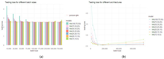 Figure 6. Performance of the different models under the initial step of approach 1, under varying batch sizes: (a) testing loss for the Poisson NN models under different architectures. The red line shows the testing loss for the Poisson regression model; (b) change in the testing loss for the Poisson NN models under different architectures as the batch size increases.All models, irrespective of their level of complexity, performed well with a batch size of 175,000. As anticipated, complex models had a higher testing loss with smaller batch sizes due to over-fitting. In general, the testing loss presented a decreasing trend for all considered models as the batch size increased from 10,000 to 175,000. For batch sizes greater than 175,000, both testing loss and learning loss for simpler models started to rise. This indicates under-fitting and shows that for batch sizes greater than 175,000, the complexity of simpler models with fewer neurons in the hidden layers is insufficient to fit the data effectively. Hence, this analysis suggested choosing a batch size of 175,000. Nevertheless, as all models had a comparable testing loss for batch size 175,000, three of the simpler models (NN (25,20,15), NN (20,15,10), and NN (15,10,5)) were considered further for identifying the optimal number of epochs.
 - Step 2: in order to find the optimal number of epochs, the NN (25,20,15), NN (20,15,10), and NN (15,10,5) models were fit using different choices of epochs (100, 250, 500, 1000, 1500, and 2000), keeping the batch size fixed at 175,000. The results of these models are given in Table 4.
Table 4. The testing loss, learning loss, and portfolio average of the Poisson neural network models with (25,20,15), (20,15,10), and (15,10,5) architectures for different choices of epochs.
For the models considered in step 2, the testing loss was lowest when the number of epochs was 1500. Hence, the combination of the batch size equal to 175,000 and 1500 epochs was deemed optimal under this approach.
Approach 2: epochs number is varied, keeping the batch size fixed; then, for the epochs number giving the best performance, different batch sizes are considered. The same steps as those followed in Approach 1 were carried out under this approach as well but in an alternate order. Model architectures, batch sizes, and numbers of epochs are also the same as in Approach 1.
- Step 1: we now initially alter the number of epochs, keeping the batch size fixed at 30,000. The results of this step are given in Table A6. For all considered model architectures, except for NN (100,75,50), the testing loss was lower than that for the Poisson regression model, when the number of epochs was 250. Moreover, the testing loss was lowest for all considered model architectures when the number of epochs was 250 (see Figure 7). Hence, the number of epochs was chosen as 250.
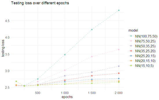 Figure 7. Change in the testing (out-of-sample) loss for Poisson neural network models with different architectures as epochs increase.
 - Step 2: For all model architectures other than (100,75,50), different batch sizes were considered with the number of epochs fixed at 250. The results are given in Table A7 and Table A8 and illustrated in Figure 8. With a batch size of 30,000, all models, except for NN (15,10,5), had testing losses lower than that for the Poisson regression model. When the batch size increased to 50,000, the NN (50,35,25) also had a similar testing loss. However, a batch size of 30,000 was chosen, as all models performed well under this choice. The combination of a batch size of 30,000 and 250 epochs was deemed optimal under the second approach.
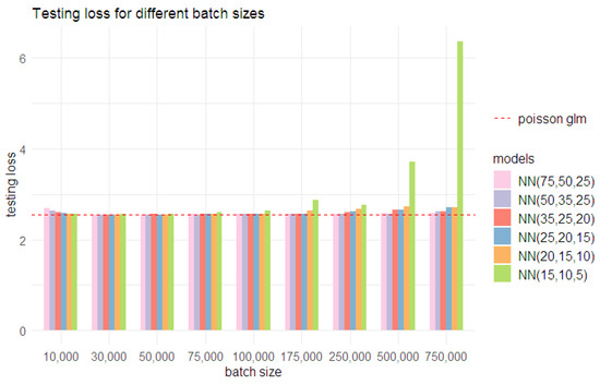 Figure 8. Change in the deviance testing (out-of-sample) loss for the Poisson neural network models with different architectures as batch size increases.
4.2.1. Comparison of Approaches
The two approaches yielded different combinations of batch sizes and epochs. Under Approach 1, the best batch size and epoch number combination was (175,000, 1500), whereas Approach 2 identified (30,000, 250) as the best combination. In order to compare these combinations, results from 50 separate calibrations with different starting points for GDM were considered for the NN (30,25,20), NN (25,20,15), NN (20,15,10), and NN (15,10,5) models (see Figure 9). The motivation behind considering different calibrations is the inherent randomness in the results of neural network models. Several aspects of the neural network model fitting contribute to this randomness and are discussed in detail in Section 6.2. Different calibrations were implemented by altering the seed value for the random number generator, which determines the initial value of model weights under GDM (see Section 6.2 for more details).
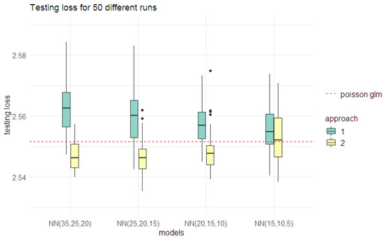
Figure 9.
Performance from 50 different calibrations for Poisson NN models under different architectures on testing data set, for the best combination of batch sizes and epochs identified in Approach 1 (175,000, 1500) and Approach 2 (30,000, 250). The horizontal red line shows the deviance loss value for the Poisson regression model.
The graphs clearly show that the combination of a batch size of 30,000 and 250 epochs performs better than a batch size of 175,000 and 1500 epochs, in terms of testing loss. The results also indicate that both (25,20,10) and (20,15,10) architectures have similar predictive performances. Hence, we consider both these architectures while investigating additional model improvements discussed in the following section.
5. Model Improvements
5.1. Approaches for Preventing Over-Fitting
One of the most significant aspects that need to be addressed while training a neural-network model is the overfitting of the model to the learning set, , which may potentially affect the predictive performance of the model. Three of the most commonly used approaches for preventing over-fitting were considered here, i.e., regularisation, early stopping, and dropout. For comparing the different improvement approaches, Poisson NN models with (25,20,10) and (20,15,10) architectures were used.
5.1.1. Regularisation
Under this approach, a penalty function is considered for the loss function, controlled by a regularisation parameter that is added to the network parameters. Following (Ferrario et al. 2020), the modified loss function for the Poisson NN is given by
where is the regularisation parameter and is the subset of network parameters considered for regularisation; is the -norm and gives . Ridge regularisation was selected over LASSO (least absolute shrinkage and selection operator regression) regularisation , as the former penalises the parameters depending upon their values and not on the same scale (Ferrario et al. 2020). Following the literature, Hastie et al. (2009) and Ferrario et al. (2020), regularisation was applied to all network parameters except for the intercepts and the last output layer. The main criticism that regularisation faces is that it is heavily influenced by the choice of the regularisation parameter. For each of the (25,20,10) and (20,15,10) architectures, four choices of the regularisation parameter were considered (, , and ) and the results are shown in Table 5 (see Listing A2 for the sample code).
Table 5.
Testing loss, learning loss, and portfolio average of the Poisson neural network models ((20,15,10), and (25,20,15) architectures) with regularisation (), and without regularisation ().
From the results, it is evident that for both model architectures, the testing loss decreased (improvement in predictive performance) when the value decreased from to . Nevertheless, for , both architectures had the same testing loss as that of the model without regularisation, indicating non-improvement of the predictive performance under regularisation. In order to further assess the effectiveness of regularisation while accounting for the inherent randomness in the results, multiple calibrations of both architectures were considered with (see Section 5.1.4).
5.1.2. Early Stopping
Generally, a neural network model starts to over-fit after a particular number of epochs. This is related to work in Section 4.2 on identifying the ideal number of epochs for a given batch size. The logic behind the early-stopping approach is to identify the ideal number of epochs above which the model starts to over-fit. In other words, the aim is to identify the number of epochs beyond which the validation loss starts to increase since an increase in validation loss indicates over-fitting of the model. Numerous ways of implementing early stopping exist, the details of which are discussed by Prechelt (1998). Our implementation employs a callback approach, which initially lets the model train for a large epoch. When the training is over, the model weights that gave the lowest value for the loss function on the validation set, are retrieved.
The early-stopping approach was implemented for both (25,20,15) and (20,15,10) architectures with a batch size of 30,000 and 1000 epochs. As anticipated, the models with early stopping performed better (see Table 6). For both model architectures, the ideal number of epochs that gave the best validation loss was around 250 (231 for (25,20,15) and 272 for (20,15,10)). Both models gave similar results as that of the already identified choice of 30,000 batch size and 250 epochs. The results indicate that the early-stopping approach is desirable over the version without early stopping (see Listing A3 for sample code). In the current context, since the early stopping was implemented using the callback approach, this overcomes the hurdle of identifying the optimal number of epochs and allows to have an arbitrarily large number of epochs (e.g., 500 epochs).
Table 6.
The testing loss, learning loss, and portfolio average of the Poisson neural network models ((20,15,10), and (25,20,15) architectures) with and without early stopping.
5.1.3. Dropout
Under this approach, for each step of the gradient descent (50 GDM steps within each of the 250 epochs), each neuron is dropped with a probability p, independently of other neurons creating a thinned network. The model weights are shared among the different thinned networks considered and make up the final unthinned neural net. In other words, for a GDM step involving thinned network, the gradient of the weights of the dropped neurons is zero Srivastava et al. (2014). See Figure 10 for a sample representation of the dropout process for a NN (20,15,10) architecture.
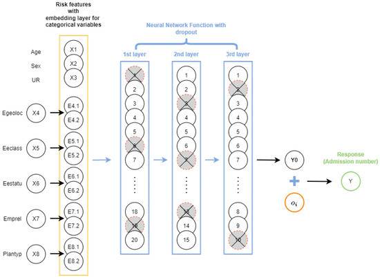
Figure 10.
An illustration of dropout process for a sample NN model with three hidden layers and 20,15,10 neurons in each layer. The gray crossed-out circles in each layer represent the neurons that were randomly dropped with probability p.
A fixed dropout rate was used for neurons in all three layers. Dropout rates of , and were considered for both model architectures. The results are shown in Table 7. When the dropout rate was , the testing loss for the (25,20,15) architecture was similar to that of the implementation without dropout, whereas for the (20,15,10) architecture, the testing loss decreased (see Listing A4 for sample code). The portfolio average for all the models with dropout is slightly different from the data indicating bias at the portfolio level (see Section 6.1 for more details on the portfolio level bias of NN models and approaches for addressing it). Since the dropout rate of performed better in comparison to , and , the former was adopted for further comparison where the randomness in the model results is also taken into consideration (see Section 5.1.4).
Table 7.
Testing loss and learning loss of the Poisson neural network models ((20,15,10) and (25,20,15) architecture) with dropout rates of .
5.1.4. Comparison of Model Improvement Approaches for Avoiding Over-Fitting
The model improvement approaches discussed above are subject to the inherent randomness in neural network training. Hence, for comparing the different approaches, 50 different calibrations were considered under each approach for both (25,20,15) and (20,15,10) architectures. The results from these different runs are illustrated in Figure 11.
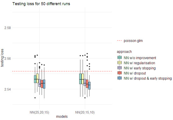
Figure 11.
Performance from 50 different calibrations of the Poisson NN model under (25,20,15) and (20,15,10) architectures on testing and learning data sets for different model improvement approaches.
Comparisons among these approaches indicated that the early stopping and dropout approaches significantly improved predictive performance. Since both approaches can be applied on the same run, it was decided to adopt both simultaneously as well. For the (25,20,15) architecture, the combination of dropout and early-stopping approaches had a similar performance as that of the two approaches when applied individually. In contrast, the (20,15,10) architecture showed improvement in the predictive performance when both approaches were applied simultaneously (see Figure 11). Hence, it was decided to proceed by adopting the combined improvement approach (early stopping and dropout).
6. Negative Binomial Neural Network Models
A comparison was carried out between the different models under Poisson and negative binomial distribution assumptions. For the network-based models, a single calibration with the combined improvement approach (early stopping and dropout) was considered to directly compare with the regression models (see Table 8). For the network-based models,(25,20,15) and (20,15,10) architectures were used with a batch size of 30,000 and 500 epochs for training the model.
Table 8.
Testing loss, learning loss, portfolio average of regression, and network-based models under the Poisson and negative binomial distributional assumptions.
The models under the negative binomial distribution assumption show better predictive performance than those under the Poisson assumption. The main difference between the models under Poisson and negative binomial assumption is the additional dispersion parameter in the negative binomial distribution. The dispersion parameter is not trained as part of the neural network model fitting and is considered separately. For training the network-based models, the dispersion parameter determined from the negative binomial regression model is used as the initial value, and the parameter is adjusted once separately after the first round of model training. The adjustment factor used to update the dispersion parameter is the ratio between the testing loss of the best neural network model and the regression model. Once the dispersion parameter is modified by multiplying with the adjustment factor, the model is freshly trained using the new value of the dispersion parameter.
From the results shown in Table 8, it is evident that the models under the negative binomial distribution assumption have lower testing loss indicating a much better predictive performance compared to models under the Poisson assumption. It is true for NN and CANN models of 25,20,15 and 20,15,10 architectures. The results also show that the CANN model performed better than the NN model under the negative binomial assumption for both 25,20,15, and 20,15,10 architectures. The same is true for 20,15,10 architecture under the Poisson assumption. For the 25,20,15 architecture, the Poisson NN model had a slightly lower testing loss than the Poisson CANN model. The portfolio average from the different network-based models was slightly different compared to the actual data. This points toward the network-based model’s failure to balance property at the portfolio level and is discussed in the section below.
6.1. Bias Regularisation
One main criticism faced by neural network models is that the balance property fails to hold on a population level: although the model gives accurate results on granular individual-level data, unbiasedness (or the balance property) fails on a portfolio level. In actuarial applications, this presents an important concern as the model can potentially lead to substantial mispricing at a population level. The root cause is the limited number of steps in gradient descent algorithms, which may restrict the parameter estimates from reaching the critical points of the Poisson deviance loss function Wüthrich (2020). For models under the negative binomial distributional assumption, the adopted log link function (which is not the canonical link function for the negative binomial distribution), can also contribute to bias in the results (Hilbe 2011).
A common bias regularisation approach is to adjust the intercept in the linear function from the last layer of the neural network, which can be implemented by multiplying the results with a constant c given by
where is the mean of the predicted values and is the mean of the observed admission numbers (Tzougas and Li 2021). This will ensure that the means of the modified predicted values are the same as the means of the observed values , such as
As an alternative approach, the GLM regularisation method was also considered. Under this approach, a GLM is added after the last hidden layer in the neural network. In essence, the neural network acts as a pre-process and the output from the last hidden layer is used to fit a GLM to predict the response. The last hidden layer is considered a learned representation of the feature space created by the network
which could be viewed as a new augmented data set for modelling admission counts with n being the number of records in the original data set (Ferrario et al. 2020). In other words, the GLM produces IWLS estimates for the weights in the last layer, thereby ensuring unbiasedness and balance. The sample code for implementing this approach is given in Listing A5. For further discussion regarding the portfolio level unbalance of network results and details regarding the different bias regularisation approaches, we refer to Wüthrich (2021) and Wüthrich (2020). The GLM bias regularisation approach was considered using NN (20,15,10) and CANN (20,15,10) models under the negative binomial distribution assumption. This presents room for further potential improvement due to the choice of the log link function in the regression implemented for bias regularisation. Hence, the simple bias regularisation approach was also adopted, together with the regression bias regularisation method. In particular, for both the NN and CANN models, the bias regularisation was implemented by extracting their last hidden layers and feeding them into the corresponding negative binomial regression models for which their intercepts were adjusted in order to control the portfolio bias. Moreover, not that the bias regularisation approaches were applied in addition to the model improvement approaches of early stopping and dropout, with a batch size of 30,000 and 500 epochs. Table 9 shows the performance of the different models with and without bias-regularisation. Bias-regularisation has a clear impact, with the portfolio average of the relevant methods being the same as that of the observed data.
Table 9.
Testing loss, learning loss, and portfolio average of regression and network-based models under negative binomial distributional assumptions with and without bias regularisation.
6.2. Nagging Predictor
As mentioned in Section 4.2.1, one of the main issues associated with neural network models is that results can vary among repeated runs. Aspects that can bring out this randomness are discussed in detail by Richman and Wüthrich (2020), and can include:
- The split of the learning data into training and validation sets;
- The split of the training data into mini-batches;
- Model initialisation.
These aspects are influenced by the choice of a random seed value for running the associated algorithms, and different seed values can potentially give slightly different results. Although the differences might be small, they should not be ignored in the context of applications of incidence rate models. The nagging predictor proposed by Richman and Wüthrich (2020) acts as a sensible approach to tackle this. The approach acts similar to the traditional bagging and aggregating approach (bagging), but without re-sampling. In other words, the aggregation occurs over the network, i.e., over different calibrations (seed values) rather than by re-sampling. The data composition in terms of the split between learning and testing data remains the same for all the calibrations, whereas the aspects of randomness, such as the ones mentioned above, vary. For the ith observation in the out-of-sample data, the nagging predictor is given by
where is the predictor obtained for the ith observation with the tth network calibration (e.g., as given in Equation (12)) and M is the number of calibrations (seed) values considered. The testing (out-of-sample) loss for the nagging predictors is given by:
where n is the number of observations in the testing data set and represents the unit deviance. The nagging predictor approach was applied on top of the already identified improvement approaches (early stopping and dropout) and bias regularisation. The nagging predictors for were calculated for both the NN and CANN models under the negative binomial distributional assumption. Due to computational limitations, we only considered a (20,15,10) architecture for the NN and CANN models, and the results are shown in Table 10 and illustrated in Figure 12.
Table 10.
Testing loss, learning loss, and portfolio average of the nagging predictor (M = 50) for the NN (20,15,10) and CANN (20,15,10) models under the negative binomial distributional assumption.
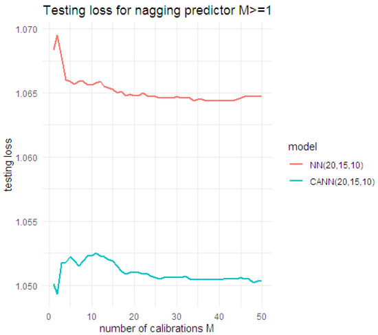
Figure 12.
Testing loss for the nagging predictors under the negative binomial NN and CANN models, using (20,15,10) architecture.
The results suggest that the nagging predictor under the CANN approach performs better than the NN approach in terms of testing loss. Moreover, under both the NN and CANN approaches, as M increases, the testing loss starts to converge to a stabilised value, demonstrating a reduction in the variability of the prediction outcomes.
7. -Fold Validation
In this section, we address the issue of potential variations in the NN model results, arising from the choice to split the data into learning and testing sets. The nagging predictor, presented in Section 6.2, does not account for this variability as it considers only those sources of randomness that arise once this split is done. Here, we consider a k-fold cross-validation approach to analyse the impact of the learning/testing split on the results and compare the performance of different models. Under the k-fold cross-validation approach introduced by Geisser (1975), the full data set is initially split into k roughly equal sets. The models under consideration are then trained using the set and validated/evaluated using the remaining set. The process is then repeated k times, altering the choice of validation set (Jung (2018)). In the current context, The value of k was set as to maintain the 90:10 split of learning and testing data. Here, we used cross-validation as a model selection procedure as discussed by Arlot and Celisse (2010) and not for training the model. The different models were compared using the average deviance loss value from the 10 folds (e.g., as in Equation (17)). As the models under the negative binomial distribution assumption demonstrated better predictive performances in our earlier analysis, compared to those under the Poisson assumption, only the former were considered in the k-fold validation. A nagging predictor (), together with the model improvement approaches discussed earlier (early stopping and dropout), was considered here for the network-based models. Bias regularisation was also applied, implementing both approaches as described in Section 6.1. The average testing and learning loss over the ten different folds are given in Table 11.
Table 11.
Average of testing loss, learning loss, and portfolio average of regression and network-based models under negative binomial distributional assumptions from the 10 different folds.
The results from the cross-validation indicate that the NN performed better than the regression and CANN models.
8. Concluding Remarks
In this research, we developed an ensemble of models for predicting the rate of admissions related to respiratory diseases in an insured US population. The results indicate that the neural network-based models have better predictive performances compared to traditional GLM-type models. A potential reason for this may be the ability of neural network models to capture possible interactions of non-multiplicative types between the different features. Although, in principle, these interactions could also be captured in GLM-type models, they must be identified and specified explicitly within the model. Adapting traditional approaches based on methods, such as step-wise Akaike information criterion (AIC) or Bayesian information criterion (BIC) for identifying relevant interactions, can be tedious and time-consuming for complex and large data sets, as in this case. Our k-fold cross-validation indicated that under an underlying negative binomial distributional assumption, the NN models gave better predictive performances, as determined by the testing data loss, than the GLM-type and CANN models. The better performances of the NN models compared to the CANN models could be partly due to the latter not involving training processes for the regression parts of the models.
The comprehensive nature of the developed models allows them to be extended with ease for modelling admission rates for other diseases, or other data in similar contexts and applications. The additional model improvement approaches, such as early stopping and dropout, further improved the predictive performances of the models. The nagging predictor addresses the inherent randomness in neural network results, and the adapted bias regularisation approach effectively resolved the population-level bias in the model results.
A potentially interesting line of further research is to develop zero-inflated versions of the NN-based models considered in this study, motivated by a high concentration of zeros in data of this nature. Furthermore, the development of hyperparameter tuning algorithms that can determine a range of different hyperparameters under a systematic search approach would be beneficial, especially in the context of large volumes of data involving high computational costs.
Finally, it should be noted that although NN-based models automatically capture general and complex interaction effects among features, their outputs are not easy to interpret, and variable selections are cumbersome. Therefore, a fruitful research avenue is to consider recently developed explainable artificial intelligence (XAI) approaches for interpreting the results from network-based models. For instance, Shapley Additive exPlanation (SHAP), local interpretable model-agnostic explanations (LIME), and particularly the LocalGLMnet methods are some promising XAI approaches that could be considered. The LocalGLMnet developed by Richman and Wüthrich (2022) proposes new network architectures that share similar features with GLM-type models without compromising their predictive performances. In the context of the health data considered in this paper, such approaches can help toward deriving actionable data insights that can potentially guide healthcare policies and intervention efforts, as well as the development and management of relevant insurance products.
Author Contributions
Conceptualization, G.S., G.T., and A.S.M.; methodology, G.S., G.T., and A.S.M.; software, A.J.; formal analysis, A.J.; investigation, A.J.; data curation, A.J.; writing—original draft preparation, A.J.; writing—review and editing, A.J., G.S., and G.T.; visualization, A.J.; supervision, G.S., G.T., and A.S.M.; project administration, G.S.; funding acquisition, G.S. All authors have read and agreed to the published version of the manuscript.
Funding
This research was funded by the Society of Actuaries, https://www.soa.org (accessed on 19 October 2021), under a CAE research grant on “Predictive modelling for medical morbidity trends related to insurance”.
Institutional Review Board Statement
Not applicable.
Informed Consent Statement
Not applicable.
Data Availability Statement
Restrictions apply to the availability of these data. We are unable to provide the data due to the data use agreement with Merative, who provided the data.
Acknowledgments
Certain data used in this study were supplied by Merative as part of one or more Merative MarketScan Research Databases. The analyses, interpretations, or conclusions based on these data are solely those of the authors and not Merative. We would also like to thank Ian Duncan of the University of California, Santa Barbara for his immense support and guidance. Finally, we thank the two anonymous reviewers for their very helpful comments and suggestions, which have significantly improved this article.
Conflicts of Interest
The authors declare no conflict of interest.
Abbreviations
The following abbreviations are used in this manuscript:
| CANN | Combined Actuarial Neural Network |
| CRD | Chronic respiratory diseases |
| COPD | Chronic obstructive pulmonary disease |
| GLM | Generalized linear model |
| BUGS | Bayesian inference Using Gibbs Sampling |
| MTPL | French motor third-party liability insurance |
| NN | Neural network |
| FFNN | Feed-forward neural network |
| ICD | International Statistical Classification of Diseases |
| GDM | Gradient descent methods |
| MSA | Metropolitan Statistical Area |
| XAI | Explainable Artificial Intelligence |
Appendix A
Appendix A.1. ICD Chapters and Variable Lookup Tables
Table A1.
Chapter-wise grouping of diagnosis codes for ICD-10 CDC (2016).
Table A1.
Chapter-wise grouping of diagnosis codes for ICD-10 CDC (2016).
| Chapter | Codes | Title |
|---|---|---|
| 1 | A00–B99 | Certain infectious and parasitic diseases |
| 2 | C00–D49 | Neoplasms |
| 3 | D50–D89 | Diseases of the blood, blood-forming organs, and certain disorders involving the immune mechanism |
| 4 | E00–E89 | Endocrine, nutritional, and metabolic diseases |
| 5 | F01–F99 | Mental and behavioral disorders |
| 6 | G00–G99 | Diseases of the nervous system |
| 7 | H00–H59 | Diseases of the eye and adnexa |
| 8 | H60–H95 | Diseases of the ear and mastoid process |
| 9 | I00–I99 | Diseases of the circulatory system |
| 10 | J00–J99 | Diseases of the respiratory system |
| 11 | K00–K95 | Diseases of the digestive system |
| 12 | L00–L99 | Diseases of the skin and subcutaneous tissue |
| 13 | M00–M99 | Diseases of the musculoskeletal system and connective tissue |
| 14 | N00–N99 | Diseases of the genitourinary system |
| 15 | O00–O9A | Pregnancy, childbirth, and the puerperium |
| 16 | P00–P96 | Certain conditions originating in the perinatal period |
| 17 | Q00–Q99 | Congenital malformations, deformations, and chromosomal abnormalities |
| 18 | R00–R99 | Symptoms, signs, and abnormal clinical and laboratory findings not classified elsewhere |
| 19 | S00–T88 | Injury, poisoning, and certain other consequences of external causes |
| 20 | V00–Y99 | External causes of morbidity and mortality |
| 21 | Z00–Z99 | Factors influencing health status and contact with health services |
Table A2.
Lookup table for EGEOLOC variables.
Table A2.
Lookup table for EGEOLOC variables.
| Value | Description |
|---|---|
| 1 | Nation, unknown region |
| 4 | Connecticut |
| 5 | Maine |
| 6 | Massachusetts |
| 7 | New Hampshire |
| 8 | Rhode Island |
| 9 | Vermont |
| 11 | New Jersey |
| 12 | New York |
| 13 | Pennsylvania |
| 16 | Illinois |
| 17 | Indiana |
| 18 | Michigan |
| 19 | Ohio |
| 20 | Wisconsin |
| 22 | Iowa |
| 23 | Kansas |
| 24 | Minnesota |
| 25 | Missouri |
| 26 | Nebraska |
| 27 | North Dakota |
| 28 | South Dakota |
| 31 | Washington, DC |
| 32 | Delaware |
| 33 | Florida |
| 34 | Georgia |
| 35 | Maryland |
| 36 | North Carolina |
| 37 | South Carolina |
| 38 | Virginia |
| 39 | West Virginia |
| 41 | Alabama |
| 42 | Kentucky |
| 43 | Mississippi |
| 44 | Tennessee |
| 46 | Arkansas |
| 47 | Louisiana |
| 48 | Oklahoma |
| 49 | Texas |
| 52 | Arizona |
| 53 | Colorado |
| 54 | Idaho |
| 55 | Montana |
| 56 | Nevada |
| 57 | New Mexico |
| 58 | Utah |
| 59 | Wyoming |
| 61 | Alaska |
| 62 | California |
| 63 | Hawaii |
| 64 | Oregon |
| 65 | Washington |
| 97 | Puerto Rico |
Table A3.
Details regarding the characteristics of different plan types.
Table A3.
Details regarding the characteristics of different plan types.
| PLANTYP | Incentive to Use Certain Provider | Primary Care Physician (PCP) Assigned? | Referrals from PCP to Specialists Required? | Out-of-Network Services Covered? | Partially or Fully Capitated? |
|---|---|---|---|---|---|
| 2. Comprehensive plan | No | No | n/a | n/a | No |
| 3. Exclusive provider organization plan | Yes | Yes | Yes | No | No |
| 4. Health maintenance organization plan | Yes | Yes | Yes | No | Yes |
| 5. Non-capitated (non-cap) point-of-service plan | Yes | Yes | Yes | Yes | No |
| 6. Preferred provider organization plan | Yes | No | n/a | Yes | No |
| 7. Capitated (Cap) or partially capitated (part cap) point-of-service plan | Yes | Yes | Yes | Yes | Yes |
| 8. Consumer-driven health plan | Varies | No | n/a | Varies | No |
| 9. High-Deductible health plan | Varies | No | n/a | Varies | No |
Appendix A.2. Selection of Batch Size and Epochs
Table A4.
The testing loss, learning loss, and portfolio average of Poisson regression model and the Poisson neural network models with (100,75,50), (75,50,25), (50,35,25), (35,25,20), (25,20,15), (20,15,10), and (15,10,5) architectures for 1000 epochs, and batch sizes 10,000 and 30,000.
Table A4.
The testing loss, learning loss, and portfolio average of Poisson regression model and the Poisson neural network models with (100,75,50), (75,50,25), (50,35,25), (35,25,20), (25,20,15), (20,15,10), and (15,10,5) architectures for 1000 epochs, and batch sizes 10,000 and 30,000.
| Model | Batch Size | Learning Loss | Testing Loss | Portfolio Average |
|---|---|---|---|---|
| Data | 0.0027 | |||
| Pois. GLM | 2.6811 | 2.5516 | 0.0027 | |
| NN (100,75,50) | 10,000 | 2.0815 | 4.3194 | 0.0027 |
| NN (75,50,25) | 10,000 | 2.2348 | 3.3182 | 0.003 |
| NN (50,35,25) | 10,000 | 2.3546 | 3.0803 | 0.0029 |
| NN (35,25,20) | 10,000 | 2.4291 | 2.9139 | 0.0028 |
| NN (25,20,15) | 10,000 | 2.5097 | 2.8273 | 0.0029 |
| NN (20,15,10) | 10,000 | 2.5533 | 2.6676 | 0.0028 |
| NN (15,10,5) | 10,000 | 2.5902 | 2.6593 | 0.0028 |
| NN (100,75,50) | 30,000 | 2.1473 | 3.4493 | 0.0028 |
| NN (75,50,25) | 30,000 | 2.3359 | 2.9862 | 0.0027 |
| NN (50,35,25) | 30,000 | 2.4454 | 2.8612 | 0.0028 |
| NN (35,25,20) | 30,000 | 2.5116 | 2.6836 | 0.0028 |
| NN (25,20,15) | 30,000 | 2.5618 | 2.6794 | 0.0027 |
| NN (20,15,10) | 30,000 | 2.5917 | 2.6164 | 0.0026 |
| NN (15,10,5) | 30,000 | 2.619 | 2.5962 | 0.0026 |
Table A5.
The testing loss, learning loss, and portfolio average of the Poisson neural network models with (100,75,50), (75,50,25), (50,35,25), (35,25,20), (25,20,15), (20,15,10), and (15,10,5) architectures for 1000 epochs, and for batch sizes 50,000, 75,000, 100,000, 175,000, 250,000, 500,000, and 750,000.
| Model | Batch Size | Learning Loss | Testing Loss | Portfolio Average |
|---|---|---|---|---|
| NN (100,75,50) | 50,000 | 2.2604 | 3.2272 | 0.0029 |
| NN (75,50,25) | 50,000 | 2.4708 | 2.7257 | 0.0028 |
| NN (50,35,25) | 50,000 | 2.5367 | 2.6943 | 0.0028 |
| NN (35,25,20) | 50,000 | 2.5768 | 2.634 | 0.0029 |
| NN (25,20,15) | 50,000 | 2.6049 | 2.6244 | 0.0029 |
| NN (20,15,10) | 50,000 | 2.6146 | 2.6135 | 0.0029 |
| NN (15,10,5) | 50,000 | 2.6316 | 2.5788 | 0.0028 |
| NN (100,75,50) | 75,000 | 2.4316 | 2.8451 | 0.0031 |
| NN (75,50,25) | 75,000 | 2.5442 | 2.6493 | 0.0028 |
| NN (50,35,25) | 75,000 | 2.5761 | 2.635 | 0.0029 |
| NN (35,25,20) | 75,000 | 2.6098 | 2.601 | 0.0029 |
| NN (25,20,15) | 75,000 | 2.6376 | 2.5731 | 0.0027 |
| NN (20,15,10) | 75,000 | 2.638 | 2.5725 | 0.0027 |
| NN (15,10,5) | 75,000 | 2.6443 | 2.5701 | 0.0027 |
| NN (100,75,50) | 100,000 | 2.5945 | 2.6077 | 0.0029 |
| NN (75,50,25) | 100,000 | 2.6057 | 2.5973 | 0.0029 |
| NN (50,35,25) | 100,000 | 2.6376 | 2.564 | 0.0027 |
| NN (35,25,20) | 100,000 | 2.6492 | 2.545 | 0.0027 |
| NN (25,20,15) | 100,000 | 2.6514 | 2.5559 | 0.0028 |
| NN (20,15,10) | 100,000 | 2.6485 | 2.5516 | 0.0027 |
| NN (15,10,5) | 100,000 | 2.6551 | 2.548 | 0.0026 |
| NN (100,75,50) | 175,000 | 2.6591 | 2.5389 | 0.0028 |
| NN (75,50,25) | 175,000 | 2.6635 | 2.5484 | 0.0028 |
| NN (50,35,25) | 175,000 | 2.6666 | 2.5642 | 0.003 |
| NN (35,25,20) | 175,000 | 2.6725 | 2.5597 | 0.0029 |
| NN (25,20,15) | 175,000 | 2.6613 | 2.5418 | 0.0028 |
| NN (20,15,10) | 175,000 | 2.6662 | 2.5525 | 0.0028 |
| NN (15,10,5) | 175,000 | 2.665 | 2.5492 | 0.0028 |
| NN (100,75,50) | 250,000 | 2.6743 | 2.5565 | 0.0027 |
| NN (75,50,25) | 250,000 | 2.6757 | 2.5581 | 0.0028 |
| NN (50,35,25) | 250,000 | 2.6754 | 2.5542 | 0.0028 |
| NN (35,25,20) | 250,000 | 2.6777 | 2.5579 | 0.0028 |
| NN (25,20,15) | 250,000 | 2.6767 | 2.5592 | 0.0028 |
| NN (20,15,10) | 250,000 | 2.6836 | 2.5612 | 0.0028 |
| NN (15,10,5) | 250,000 | 2.7349 | 2.6092 | 0.0032 |
| NN (100,75,50) | 500,000 | 2.6823 | 2.5558 | 0.0028 |
| NN (75,50,25) | 500,000 | 2.6871 | 2.5631 | 0.0028 |
| NN (50,35,25) | 500,000 | 2.6877 | 2.5603 | 0.0028 |
| NN (35,25,20) | 500,000 | 2.69 | 2.564 | 0.0028 |
| NN (25,20,15) | 500,000 | 2.6934 | 2.5642 | 0.0028 |
| NN (20,15,10) | 500,000 | 2.7624 | 2.6288 | 0.0029 |
| NN (15,10,5) | 500,000 | 2.8025 | 2.6763 | 0.0029 |
| NN (100,75,50) | 750,000 | 2.6825 | 2.5552 | 0.0028 |
| NN (75,50,25) | 750,000 | 2.6892 | 2.5605 | 0.0028 |
| NN (50,35,25) | 750,000 | 2.6889 | 2.56 | 0.0028 |
| NN (35,25,20) | 750,000 | 2.7007 | 2.5684 | 0.0028 |
| NN (25,20,15) | 750,000 | 2.7646 | 2.6296 | 0.003 |
| NN (20,15,10) | 750,000 | 2.7947 | 2.6707 | 0.0033 |
| NN (15,10,5) | 750,000 | 2.9142 | 2.8013 | 0.0051 |
Table A6.
The testing loss, learning loss, and portfolio average of the Poisson neural network models with different architectures for different choices of epochs.
Table A6.
The testing loss, learning loss, and portfolio average of the Poisson neural network models with different architectures for different choices of epochs.
| Model | Epochs | Learning Loss | Testing Loss | Portfolio Average |
|---|---|---|---|---|
| Data | 0.0027 | |||
| Pois.GLM | 2.6811 | 2.5516 | 0.0027 | |
| NN (100,75,50) | 100 | 2.6866 | 2.563 | 0.0031 |
| NN (75,50,25) | 100 | 2.6836 | 2.5606 | 0.003 |
| NN (50,35,25) | 100 | 2.6869 | 2.5649 | 0.0032 |
| NN (35,25,20) | 100 | 2.6851 | 2.5611 | 0.0028 |
| NN (25,20,15) | 100 | 2.6917 | 2.568 | 0.0028 |
| NN (20,15,10) | 100 | 2.696 | 2.5687 | 0.0028 |
| NN (15,10,5) | 100 | 2.8045 | 2.6778 | 0.0029 |
| NN (100,75,50) | 250 | 2.6518 | 2.5527 | 0.0026 |
| NN (75,50,25) | 250 | 2.6589 | 2.5448 | 0.0028 |
| NN (50,35,25) | 250 | 2.6599 | 2.5454 | 0.0026 |
| NN (35,25,20) | 250 | 2.6615 | 2.5379 | 0.0028 |
| NN (25,20,15) | 250 | 2.6605 | 2.5404 | 0.0026 |
| NN (20,15,10) | 250 | 2.6627 | 2.541 | 0.0024 |
| NN (15,10,5) | 250 | 2.6618 | 2.5396 | 0.0025 |
| NN (100,75,50) | 500 | 2.4575 | 2.7481 | 0.0029 |
| NN (75,50,25) | 500 | 2.5440 | 2.6737 | 0.0028 |
| NN (50,35,25) | 500 | 2.6074 | 2.5824 | 0.0027 |
| NN (35,25,20) | 500 | 2.6256 | 2.5703 | 0.0028 |
| NN (25,20,15) | 500 | 2.6288 | 2.5703 | 0.0027 |
| NN (20,15,10) | 500 | 2.6452 | 2.5683 | 0.0028 |
| NN (15,10,5) | 500 | 2.6459 | 2.5569 | 0.0028 |
| NN (100,75,50) | 1000 | 2.1653 | 3.4808 | 0.0028 |
| NN (75,50,25) | 1000 | 2.3453 | 3.0112 | 0.0029 |
| NN (50,35,25) | 1000 | 2.4357 | 2.8469 | 0.0027 |
| NN (35,25,20) | 1000 | 2.5345 | 2.7145 | 0.0027 |
| NN (25,20,15) | 1000 | 2.5661 | 2.6647 | 0.0027 |
| NN (20,15,10) | 1000 | 2.5983 | 2.5962 | 0.0027 |
| NN (15,10,5) | 1000 | 2.6194 | 2.5996 | 0.0028 |
| NN (100,75,50) | 1500 | 2.1123 | 4.2328 | 0.0029 |
| NN (75,50,25) | 1500 | 2.2884 | 3.4217 | 0.003 |
| NN (50,35,25) | 1500 | 2.3753 | 2.9564 | 0.0029 |
| NN (35,25,20) | 1500 | 2.4651 | 2.8431 | 0.0029 |
| NN (25,20,15) | 1500 | 2.5323 | 2.7397 | 0.0028 |
| NN (20,15,10) | 1500 | 2.5565 | 2.6925 | 0.0028 |
| NN (15,10,5) | 1500 | 2.6032 | 2.6234 | 0.0027 |
| NN (100,75,50) | 2000 | 2.105 | 4.8078 | 0.0029 |
| NN (75,50,25) | 2000 | 2.2302 | 3.631 | 0.0029 |
| NN (50,35,25) | 2000 | 2.3314 | 3.1311 | 0.0029 |
| NN (35,25,20) | 2000 | 2.4312 | 2.923 | 0.0028 |
| NN (25,20,15) | 2000 | 2.4837 | 2.764 | 0.0027 |
| NN (20,15,10) | 2000 | 2.5611 | 2.6882 | 0.0026 |
| NN (15,10,5) | 2000 | 2.5997 | 2.6522 | 0.0027 |
Table A7.
The testing loss, learning loss, and portfolio average of the Poisson neural network models with different architectures for 10,000, 30,000, 50,000, 75,000, 100,000, and 175,000 batch sizes.
Table A7.
The testing loss, learning loss, and portfolio average of the Poisson neural network models with different architectures for 10,000, 30,000, 50,000, 75,000, 100,000, and 175,000 batch sizes.
| Model | Batch Size | Learning Loss | Testing Loss | Portfolio Average |
|---|---|---|---|---|
| Data | 0.0027 | |||
| Pois.GLM | 2.6811 | 2.5516 | 0.0027 | |
| NN (75,50,25) | 10,000 | 2.5453 | 2.6831 | 0.0031 |
| NN (50,35,25) | 10,000 | 2.5917 | 2.6302 | 0.003 |
| NN (35,25,20) | 10,000 | 2.6184 | 2.6045 | 0.003 |
| NN (25,20,15) | 10,000 | 2.6305 | 2.5834 | 0.0029 |
| NN (20,15,10) | 10,000 | 2.631 | 2.574 | 0.0029 |
| NN (15,10,5) | 10,000 | 2.6469 | 2.561 | 0.0028 |
| NN (75,50,25) | 30,000 | 2.6565 | 2.5493 | 0.0028 |
| NN (50,35,25) | 30,000 | 2.6546 | 2.5515 | 0.0027 |
| NN (35,25,20) | 30,000 | 2.6594 | 2.5442 | 0.0027 |
| NN (25,20,15) | 30,000 | 2.6594 | 2.5463 | 0.0027 |
| NN (20,15,10) | 30,000 | 2.6602 | 2.5402 | 0.0025 |
| NN (15,10,5) | 30,000 | 2.6657 | 2.568 | 0.0025 |
| NN (75,50,25) | 50,000 | 2.6751 | 2.5518 | 0.0027 |
| NN (50,35,25) | 50,000 | 2.674 | 2.5484 | 0.0027 |
| NN (35,25,20) | 50,000 | 2.6748 | 2.5572 | 0.0026 |
| NN (25,20,15) | 50,000 | 2.6758 | 2.5533 | 0.0026 |
| NN (20,15,10) | 50,000 | 2.6786 | 2.556 | 0.0026 |
| NN (15,10,5) | 50,000 | 2.6824 | 2.5618 | 0.0027 |
| NN (75,50,25) | 75,000 | 2.6824 | 2.5575 | 0.0027 |
| NN (50,35,25) | 75,000 | 2.6773 | 2.5551 | 0.0027 |
| NN (35,25,20) | 75,000 | 2.6851 | 2.5633 | 0.0027 |
| NN (25,20,15) | 75,000 | 2.6857 | 2.5626 | 0.0028 |
| NN (20,15,10) | 75,000 | 2.6844 | 2.5642 | 0.0027 |
| NN (15,10,5) | 75,000 | 2.7231 | 2.5933 | 0.003 |
| NN (75,50,25) | 100,000 | 2.6839 | 2.5603 | 0.0027 |
| NN (50,35,25) | 100,000 | 2.6831 | 2.5586 | 0.0027 |
| NN (35,25,20) | 100,000 | 2.69 | 2.5652 | 0.0028 |
| NN (25,20,15) | 100,000 | 2.6877 | 2.5642 | 0.0028 |
| NN (20,15,10) | 100,000 | 2.7066 | 2.5724 | 0.0029 |
| NN (15,10,5) | 100,000 | 2.7639 | 2.6299 | 0.003 |
| NN (75,50,25) | 175,000 | 2.686 | 2.5582 | 0.0028 |
| NN (50,35,25) | 175,000 | 2.6912 | 2.5579 | 0.0028 |
| NN (35,25,20) | 175,000 | 2.6896 | 2.5591 | 0.0028 |
| NN (25,20,15) | 175,000 | 2.7061 | 2.5734 | 0.0028 |
| NN (20,15,10) | 175,000 | 2.7658 | 2.6331 | 0.0029 |
| NN (15,10,5) | 175,000 | 2.9795 | 2.8704 | 0.0059 |
Table A8.
The testing loss, learning loss, and portfolio average of the Poisson neural network models with different architectures for 250,000 and 500,000 and 750,000 batch sizes.
Table A8.
The testing loss, learning loss, and portfolio average of the Poisson neural network models with different architectures for 250,000 and 500,000 and 750,000 batch sizes.
| Model | Batch Size | Learning Loss | Testing Loss | Portfolio Average |
|---|---|---|---|---|
| NN (75,50,25) | 250,000 | 2.6985 | 2.566 | 0.0028 |
| NN (50,35,25) | 250,000 | 2.702 | 2.5674 | 0.0028 |
| NN (35,25,20) | 250,000 | 2.7312 | 2.5956 | 0.003 |
| NN (25,20,15) | 250,000 | 2.7579 | 2.6222 | 0.003 |
| NN (20,15,10) | 250,000 | 2.8054 | 2.6816 | 0.0033 |
| NN (15,10,5) | 250,000 | 2.8716 | 2.7557 | 0.0046 |
| NN (75,50,25) | 500,000 | 2.721 | 2.5869 | 0.0029 |
| NN (50,35,25) | 500,000 | 2.7048 | 2.5666 | 0.0028 |
| NN (35,25,20) | 500,000 | 2.7868 | 2.6548 | 0.003 |
| NN (25,20,15) | 500,000 | 2.7821 | 2.6511 | 0.0031 |
| NN (20,15,10) | 500,000 | 2.8502 | 2.7323 | 0.0042 |
| NN (15,10,5) | 500,000 | 3.7937 | 3.7045 | 0.0131 |
| NN (75,50,25) | 750,000 | 2.7237 | 2.5909 | 0.003 |
| NN (50,35,25) | 750,000 | 2.7492 | 2.6152 | 0.0029 |
| NN (35,25,20) | 750,000 | 2.754 | 2.6209 | 0.0032 |
| NN (25,20,15) | 750,000 | 2.8334 | 2.7084 | 0.0039 |
| NN (20,15,10) | 750,000 | 2.8275 | 2.7067 | 0.0041 |
| NN (15,10,5) | 750,000 | 6.4324 | 6.3651 | 0.0317 |
Appendix A.3. Code
| Listing A1: Code for implementing . |
 |
| Listing A2: Code for implementing ridge regularisation with . |
 |
| Listing A3: Code for implementing early stopping using callback. |
 |
| Listing A4: Code for implementing dropout with dropout rate . |
 |
| Listing A5: Code for implementing the GLM bias regularisation approach for Poisson neuralnetwork model. |
 |
References
- Allaire, Joseph J, and François Chollet. 2021. Keras: R Interface to ‘Keras’, R Package Version 2.7.0; Available online: https://CRAN.R-project.org/package=keras (accessed on 9 January 2022).
- Allaire, Joseph J., and Yuan Tang. 2021. Tensorflow: R Interface to ‘TensorFlow’, R Package Version 2.6.0; Available online: https://CRAN.R-project.org/package=tensorflow (accessed on 9 January 2022).
- Arık, Ayşe, Erengul Dodd, Andrew Cairns, and George Streftaris. 2021. Socioeconomic disparities in cancer incidence and mortality in england and the impact of age-at-diagnosis on cancer mortality. PLoS ONE 16: e0253854. [Google Scholar] [CrossRef] [PubMed]
- Arlot, Sylvain, and Alain Celisse. 2010. A survey of cross-validation procedures for model selection. Statistics Surveys 4: 40–79. [Google Scholar] [CrossRef]
- Aveyard, Paul, Min Gao, Nicola Lindson, Jamie Hartmann-Boyce, Peter Watkinson, Duncan Young, Carol A. C. Coupland, Pui San Tan, Ashley K. Clift, David Harrison, and et al. 2021. Association between pre-existing respiratory disease and its treatment, and severe COVID-19: A population cohort study. The Lancet Respiratory Medicine 9: 909–23. [Google Scholar] [CrossRef]
- Bengio, Yoshua, Réjean Ducharme, and Pascal Vincent. 2000. A neural probabilistic language model. In Advances in Neural Information Processing Systems 13. Cambridge: MIT Press. [Google Scholar]
- Blanc, Paul D., Isabella Annesi-Maesano, John R. Balmes, Kristin J. Cummings, David Fishwick, David Miedinger, Nicola Murgia, Rajen N. Naidoo, Carl J. Reynolds, Torben Sigsgaard, and et al. 2019. The occupational burden of nonmalignant respiratory diseases. an official american thoracic society and european respiratory society statement. American Journal of Respiratory and Critical Care Medicine 199: 1312–34. [Google Scholar] [CrossRef] [PubMed]
- Blier-Wong, Christopher, Hélène Cossette, Luc Lamontagne, and Etienne Marceau. 2020. Machine learning in P&C insurance: A review for pricing and reserving. Risks 9: 4. [Google Scholar] [CrossRef]
- Bousquet, Jean, Nikolai Khaltaev, and Alvaro A. Cruz. 2007. Global Surveillance, Prevention and Control of Chronic Respiratory Diseases. Geneva: World Health Organization. [Google Scholar]
- CDC. 2012. Chronic obstructive pulmonary disease among adults-United States, 2011. Morbidity and Mortality Weekly Report 61: 938–43. [Google Scholar]
- CDC. 2016. ICD-10-CM International Classification of Diseases, Tenth Revision, Clinical Modification (ICD-10-CM). Available online: https://www.cdc.gov/nchs/icd/icd-10-cm.htm (accessed on 12 December 2021).
- De Jong, Piet, and Gillian Z. Heller. 2008. Generalized Linear Models for Insurance Data. Cambridge: Cambridge University Press. [Google Scholar]
- Doney, Brent, Eva Hnizdo, Girija Syamlal, Greg Kullman, Cecil Burchfiel, Christopher J. Martin, and Priscah Mujuru. 2014. Prevalence of chronic obstructive pulmonary disease among us working adults aged 40 to 70 years: National health interview survey data 2004 to 2011. Journal of Occupational and Environmental Medicine/American College of Occupational and Environmental Medicine 56: 1088. [Google Scholar] [CrossRef]
- Dozat, Timothy. 2016. Incorporating nesterov momentum into adam. Paper presented at the 4th International Conference on Learning Representations, San Juan, Puerto Rico, May 2–4. [Google Scholar]
- Ferrario, Andrea, Alexander Noll, and Mario V. Wuthrich. 2020. Insights from inside neural networks. SSRN. Available online: https://papers.ssrn.com/sol3/papers.cfm?abstract_id=3226852 (accessed on 20 November 2021).
- Frees, Edward W. 2009. Regression Modeling with Actuarial and Financial Applications. Cambridge: Cambridge University Press. [Google Scholar]
- Geisser, Seymour. 1975. The predictive sample reuse method with applications. Journal of the American Statistical Association 70: 320–28. [Google Scholar] [CrossRef]
- Goodfellow, Ian, Yoshua Bengio, and Aaron Courville. 2016. Deep Learning. Cambridge: MIT Press. [Google Scholar]
- Haberman, Steven, and Arthur E. Renshaw. 1996. Generalized linear models and actuarial science. Journal of the Royal Statistical Society: Series D (The Statistician) 45: 407–36. [Google Scholar] [CrossRef]
- Hardin, James W., James William Hardin, Joseph M. Hilbe, and Joseph Hilbe. 2007. Generalized Linear Models and Extensions. College Station: Stata Press. [Google Scholar]
- Hastie, Trevor, Robert Tibshirani, Jerome H. Friedman, and Jerome H. Friedman. 2009. The Elements of Statistical Learning: Data Mining, Inference, and Prediction. New York: Springer, vol. 2. [Google Scholar]
- Hilbe, Joseph M. 2011. Negative Binomial Regression. Cambridge: Cambridge University Press. [Google Scholar]
- Jung, Yoonsuh. 2018. Multiple predicting k-fold cross-validation for model selection. Journal of Nonparametric Statistics 30: 197–215. [Google Scholar] [CrossRef]
- LeCun, Yann, Yoshua Bengio, and Geoffrey Hinton. 2015. Deep learning. Nature 521: 436–44. [Google Scholar] [CrossRef] [PubMed]
- Nelder, John Ashworth, and Robert W. M. Wedderburn. 1972. Generalized linear models. Journal of the Royal Statistical Society: Series A (General) 135: 370–84. [Google Scholar] [CrossRef]
- Ohlsson, Esbjörn, and Björn Johansson. 2010. Non-Life Insurance Pricing with Generalized Linear Models. Berlin: Springer, vol. 2. [Google Scholar]
- Ozkok, Erengul, George Streftaris, Howard R. Waters, and A. David Wilkie. 2014. Modelling critical illness claim diagnosis rates I: Methodology. Scandinavian Actuarial Journal 2014: 439–57. [Google Scholar] [CrossRef]
- Prechelt, Lutz. 1998. Early stopping-but when? In Neural Networks: Tricks of the Trade. Berlin: Springer, pp. 5–69. [Google Scholar]
- R Core Team. 2021. R: A Language and Environment for Statistical Computing. Vienna: R Foundation for Statistical Computing. [Google Scholar]
- Richman, Ronald, and Mario V. Wüthrich. 2020. Nagging predictors. Risks 8: 83. [Google Scholar] [CrossRef]
- Richman, Ronald, and Mario V. Wüthrich. 2021. A neural network extension of the Lee–Carter model to multiple populations. Annals of Actuarial Science 15: 346–66. [Google Scholar] [CrossRef]
- Richman, Ronald, and Mario V. Wüthrich. 2022. LocalGLMnet: Interpretable Deep Learning for Tabular Data. Scandinavian Actuarial Journal, 1–25. [Google Scholar] [CrossRef]
- Rigby, Robert A., and D. Mikis Stasinopoulos. 2005. Generalized additive models for location, scale and shape. Applied Statistics 54: 507–54. [Google Scholar] [CrossRef]
- RStudio Team. 2021. RStudio: Integrated Development Environment for R. Boston: RStudio, PBC. [Google Scholar]
- Ruder, Sebastian. 2016. An overview of gradient descent optimization algorithms. arXiv arXiv:1609.04747. [Google Scholar]
- Russell, Stuart J. 2010. Artificial Intelligence a Modern Approach. Upper Saddle River: Pearson Education, Inc. [Google Scholar]
- Schelldorfer, Jürg, and Mario V. Wuthrich. 2019. Nesting classical actuarial models into neural networks. SSRN. Available online: https://papers.ssrn.com/sol3/papers.cfm?abstract_id=3320525 (accessed on 15 December 2021).
- Srivastava, Nitish, Geoffrey Hinton, Alex Krizhevsky, Ilya Sutskever, and Ruslan Salakhutdinov. 2014. Dropout: A simple way to prevent neural networks from overfitting. The Journal of Machine Learning Research 15: 1929–58. [Google Scholar]
- Tzougas, George, and Ziyi Li. 2021. Neural Network Embedding of the Mixed Poisson Regression Model for Claim Counts. Available online: https://insurancedatascience.org/project/2021_london/ (accessed on 9 January 2022).
- WHO. 2022a. Asthma and COVID-19: Scientific Brief. Available online: https://www.who.int/publications-detail-redirect/who-2019-ncov-sci-brief-asthma-2021.1 (accessed on 19 April 2022).
- WHO. 2022b. Heath Topics-Chronic Respiratory Diseases. Available online: https://www.who.int/health-topics/chronic-respiratory-diseases#tab=tab_1 (accessed on 6 June 2022).
- Wüthrich, Mario V. 2020. Bias regularization in neural network models for general insurance pricing. European Actuarial Journal 10: 179–202. [Google Scholar] [CrossRef]
- Wüthrich, Mario V. 2021. The balance property in neural network modelling. Statistical Theory and Related Fields 6: 1–9. [Google Scholar] [CrossRef]


Publisher’s Note: MDPI stays neutral with regard to jurisdictional claims in published maps and institutional affiliations. |
© 2022 by the authors. Licensee MDPI, Basel, Switzerland. This article is an open access article distributed under the terms and conditions of the Creative Commons Attribution (CC BY) license (https://creativecommons.org/licenses/by/4.0/).