Article

Spectral Expansions for Credit Risk Modelling with Occupation Times

Department of Mathematics, Faculty of Science, Wilfrid Laurier University, 75 University Ave. West, Waterloo, ON N2L 3C5, Canada
*
Author to whom correspondence should be addressed.
Risks 2022, 10(12), 228; https://doi.org/10.3390/risks10120228
Submission received: 10 November 2022 / Revised: 21 November 2022 / Accepted: 25 November 2022 / Published: 30 November 2022

Abstract

:
We study two credit risk models with occupation time and liquidation barriers: the structural model and the hybrid model with hazard rate. The defaults within the models are characterized in accordance with Chapter 7 (a liquidation process) and Chapter 11 (a reorganization process) of the U.S. Bankruptcy Code. The models assume that credit events trigger as soon as the occupation time (the cumulative time the firm’s value process spends below some threshold level) exceeds the grace period (time allowance). The hazard rate model extends the structural occupation time models and presumes that other random factors may also lead to credit events. Both approaches allow the firm to fulfill its obligations during the grace period. We derive new closed-from pricing formulas for credit derivatives containing the (risk-neutral) probability of defaults and credit default swap (CDS) spreads as special cases, which are derived analytically via a spectral expansion methodology. Our method works for any solvable diffusion, such as the geometric Brownian motion (GBM) and several state-dependent volatility processes, including the constant elasticity of variance (CEV) model. It allows us to write the pricing formulas explicitly as infinite series that converges rapidly. We then calibrate our models (assuming that GBM governs the firm’s value) to market CDS spreads from the Total Energy company. Our calibration results show that the computations are fast, and the fit is near-perfect.

1. Introduction

Structural and reduced-form models are the two main mathematical modelling approaches to credit risk. Structural models assume that a credit event triggers based on the current firm’s value movement. Such models are linked to the debt-to-equity ratio since the higher the ratio value, the higher the firm’s risk. It is reasonable to assume that a default occurs if the firm’s value goes (or stays) below some threshold level. The Merton model Merton (1974) is one of the first structural models to analyze defaults. The firm in the Merton model defaults if the firm’s value at maturity is less than some threshold level. A significant drawback of the Merton model is that it assumes that default events can only happen at known maturity times. The Black–Cox model Black and Cox (1976) extends the Merton model by allowing the firm to default at any time before or at maturity. The firm defaults once its value hits a specific barrier.
Most of the classical structural models treat default and liquidation as the same event. For example, in the Black–Cox model and in its numerous modifications, default/liquidation occurs when the firm value reaches an absorbing low barrier. According to the U.S. bankruptcy code, a firm that is unable to manage its debt can be given the right to declare bankruptcy under Chapter 11 (a reorganization process) and then reorganize its business. If the reorganization plan fails, Chapter 11 is converted to Chapter 7 (a liquidation process), and the firm is to be liquidated. There are many recent works in which a distinction between bankruptcy and liquidation is made. See, for instance, the discussions in Moraux (2002); Nardon (2008); Galai et al. (2007); and Broadie et al. (2007). Typically, liquidation time is introduced as the first time the firm’s asset value constantly or cumulatively stayed below the bankruptcy level over a certain period of time.
Defaults in the Black–Cox model are characterized in the form of the U.S. Bankruptcy Code Chapter 7. Occupation time models Makarov et al. (2015); Makarov (2016) further extend the Black–Cox model by allowing the firm to stay below a bankruptcy barrier for a specified amount of time as some firms admit a grace period to ensure the firm would be able to fulfill its obligations during the grace period. Therefore, defaults in occupation time models are characterized per both Chapters 7 and 11 of the U.S. Bankruptcy Code. Alternatively, excursion times can be used for a temporal separation between default and liquidation Li et al. (2014). Structural models with Parisian stopping times are related to Parisian options (see Chesney et al. (1997); Haber et al. (1999)).
Reduced-form models are intensity-based models where the likelihood of a default is measured by its hazard rate. Reduced-form models lack the ability to determine defaults endogenously with the firm’s value process movements. Alfonsi and Lelong proposed in Alfonsi and Lelong (2012) a hybrid model that unifies the Black–Cox model and reduce-form models, in which default occurs based on hazard rate processes driven by the firm’s value and other exogenous factors. However, the Alfonsi–Lelong model only considers the Chapter 7 type defaults.
In this paper, we use both structural and hybrid approaches. The total value of the firm’s assets follows some diffusion process, which we call an F-diffusion. We assume that there exists a monotonic mapping that reduces the F-diffusion to a solvable X-diffusion, for which we can derive some fundamental formulas in closed form. In particular, we can obtain the joint probability density of the process value and its occupation time in the form of a spectral series expansion. The simplest example is GBM, which can be mapped to Brownian motion with drift. Although we focus on the GBM case in the numerical study, our methodology applies to a broad class of solvable diffusions.
We propose two occupation time-based models where closed-form pricing formulas for credit derivatives are derived analytically via a spectral expansion methodology. The spectral expansion method works for any solvable diffusions, including such processes as Brownian motion, the squared Bessel (SQB), the Cox–Ingersoll–Ross (CIR) and the Ornstein–Uhlenbeck (OU) processes. It is used to find closed-form credit derivative prices as a discrete expansion form that converges quickly. The first model we consider is an occupation time model in which defaults are characterized in accordance with the U.S. Bankruptcy Code Chapters 7 and 11. One of our occupation time models coincides with the model in Makarov (2016), except that we now employ the spectral expansion method. Furthermore, we derive closed-form pricing formulas for credit derivatives under this model. We also propose a new hybrid hazard rate model, which recovers the Black–Cox model and the Alfonsi–Lelong model as a particular case. Our hybrid model characterizes both Chapters 7 and 11 type defaults and contains closed-form pricing formulas for credit derivatives, leading to fast and accurate calibrations of market CDS spreads.
The paper is organized as follows. Section 2 and Section 3 present the concept of occupation time and the main results associated with occupation time processes. Section 4 states our new developments pertaining to the occupation time models that were not exploited in Makarov (2016) and yet will be helpful in later sections. Section 5 describes the hazard rate model, which extends the Black–Cox and Alfonsi–Lelong models. Section 6 and Section 7 present default probabilities and implied hazard rate functions and how they relate to one another. Section 8 entails pricing formulas for credit default swap (CDS) spreads. In Section 9, we provide the calibration procedure and results for CDS spreads (for the GBM case).

2. Occupation Time Process for Underlying Diffusion

We fix a filtered probability space ( Ω , F , P , F ) where F = { F t } t 0 is the natural filtration for ( P , F ) -Brownian motion { W t } t 0 . Let X be a one-dimensional time-homogeneous regular diffusion process1 on a state space I = ( l , r ) R with endpoints l , r satisfying l < r . The generator is defined by
G f ( x ) : = 1 2 σ 2 ( x ) f ( x ) + μ ( x ) f ( x ) = 1 m ( x ) f ( x ) s ( x ) ; x I ,
with appropriate boundary condition at the endpoints. The speed m ( x ) and scale s ( x ) densities, where s ( x ) and m ( x ) are continuous and positive for x I (see Borodin and Salminen (2002)), are defined via the drift, μ ( x ) , and diffusion, σ ( x ) , coefficient functions as follows:
s ( x ) : = exp x 2 μ ( z ) σ 2 ( z ) d z , m ( x ) : = 2 σ 2 ( x ) s ( x ) .
The diffusion X satisfies the stochastic differential equation (SDE)
d X t = μ ( X t ) d t + σ ( X t ) d W t .
An occupation time A t , + (or A t , ) is defined as the cumulative time the diffusion X I stays above (or below) the occupation level I from time 0 to time t:
A t , + : = 0 t I [ , r ) ( X s ) d s ; t 0 , I , A t , : = 0 t I ( l , ] ( X s ) d s ; t 0 , I .
The diffusion X with imposed lower and upper (regular) killings at a and b (where a < b ), respectively, is defined by
X ( a , b ) , t : = X t t < T ( a , b ) t T ( a , b ) ; X 0 = x ( a , b ) ,
where T ( a , b ) : = inf { t 0 : X t ( a , b ) } is the first exit time from the interval ( a , b ) , and denotes the cemetery (killed) state.2
Let λ be an instantaneous killing rate defined by:
λ ( X t ) : = α 1 I [ , r ) ( X t ) + α 2 I ( l , ] ( X t ) ; 0 α 1 α 2 .
Define the following process with instantaneous killing rate λ as:
X ˜ ( a , b ) , t : = X ( a , b ) , t Γ t < ξ , Γ t ξ ,
where
Γ t : = 0 t λ ( X s ) d s = α 1 A t , + + α 2 A t ,
is an F -adapted hazard process and ξ Exp ( 1 ) is an F -independent exponential random variable with unit rate. It is enough to consider only the occupation time below (i.e., α 1 = 0 ) thanks to a simple identity A t , + + A t , = t . The hazard process in (7) can be simplified to
Γ t = α 1 t + ( α 2 α 1 ) A t , .
In the remainder of this section (and the next section) we shall assume α 1 = 0 and α 2 = α 0 . We can define the transition density of the diffusion X with the instantaneous killing rate in (5):3,4
p ˜ ( a , b ) , α , ( t ; x , y ) d y : = P x X ˜ ( a , b ) , t d y = E x e α A t , ; X t d y , m t > a , M t < b ;
for t > 0 , x , y ( a , b ) , and zero otherwise, where m t : = inf 0 u t X u and M t : = sup 0 u t X u .5 Since both boundaries are NONOSC (non-oscillatory), we are in the Spectral Category I (see, e.g., Campolieti; Campolieti et al. (2013); Linetsky (2004)) and the transition density in (9) admits a discrete spectral expansion form:
p ˜ ( a , b ) , α , ( t ; x , y ) = m ( y ) n = 1 e λ ˜ n t ϕ ˜ n , α , ( x ) ϕ ˜ n , α , ( y ) ,
where { ϕ ˜ n , α , } are eigenfunctions with eigenvalues { λ ˜ n } as the set of increasing simple zeros. The explicit formulas for Brownian motion are given in Appendix A. We define the joint density of the occupation time process (below ) and the diffusion with imposed killing at endpoints a and b:
f A t , , X t ( a , b ) ( u , y x ) d u d y : = P x A t , d u , X t d y , m t > a , M t < b ,
for any u ( 0 , t ) , x , y ( a , b ) , and zero otherwise. The joint density is defective at 0 and t where
P x A t , = 0 , X t d y , m t > a , M t < b = p ( , b ) ( t ; x , y ) d y , P x A t , = t , X t d y , m t > a , M t < b = p ( a , ) ( t ; x , y ) d y .
The joint density can be obtained from the transition density in (9) by Laplace inverting with respect to α : (which can be evaluated numerically via the Gaver–Stehfest algorithm, see Cohen (2007); Gaver (1966); Stehfest (1970))
f A t , , X t ( a , b ) ( u , y x ) = L α 1 p ˜ ( a , b ) , α , ( t ; x , y ) ( u ) ; u ( 0 , t ) , x , y ( a , b ) .
The expectations of a bounded Borel function of the X-diffusion and its occupation time can be evaluated as:6
E x h ( X t ) e α A t , ; m t > a = a r h ( y ) p ˜ ( a , r ) , α , ( t ; x , y ) d y , E x h A t , , X t ; m t > a = 0 t a r h ( u , y ) f A t , , X t ( a , r ) ( u , y x ) d y d u + a h ( t , y ) p ( a , ) ( t ; x , y ) d y x ( a , ] , r h ( 0 , y ) p + ( t ; x , y ) d y x [ , r ) ,
where
p + ( t ; x , y ) d y : = P x X t d y , m t > ; x [ , r ) ,
and zero otherwise, is the transition density of X with a lower imposed killing at level .
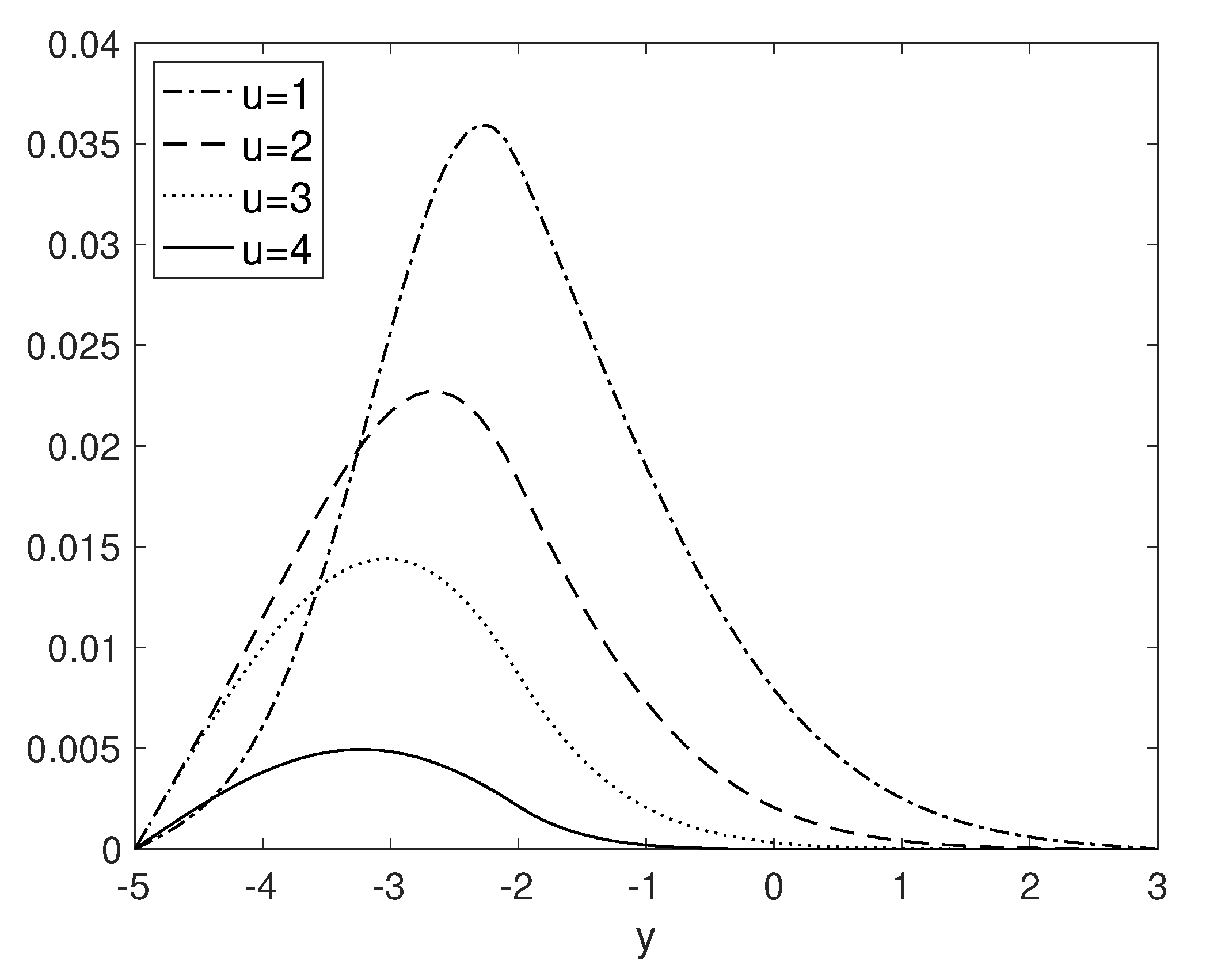
Figure 1 shows some graphs of the transition density in (9) using the truncated N-term series in (10) for the case of standard Brownian motion. The top-left graph shows that the N-term series converges with N = 8 terms in the series with a = −5, b = 3 , = 2 , α = 0.25 , and t = 1. If we increase b to 35 in the top-right graph, we can see that it requires more terms (N ≈ 40) to obtain convergence of the series. If we increase t to 5 (from the top-left to the bottom-left) we can observe that the series requires less terms to demonstrate converge. The bottom-right graph shows that p ˜ ( a , b ) , α , ( t ; x , y ) p ( a , b ) ( t ; x , y ) as α 0 and p ˜ ( a , b ) , α , ( t ; x , y ) p ( , b ) ( t ; x , y ) as α . Figure 2 shows the graph of the joint density in (11) and works well since p ˜ ( a , b ) , α , ( t ; x , y ) is a smooth function of α .

3. Occupation Time Process for F -Diffusion

Consider an F-diffusion F t : = F ( X t ) , t 0 (starting at F 0 : = F ( x ) , X 0 = x ), defined in terms of a given diffusion X where F : I D : = ( F ( l ) , F ( r ) ) , with F ( l ) : = min ( F ( l ) , F ( r ) ) and F ( r ) : = max ( F ( l ) , F ( r ) ) , is a smooth monotonic function with unique inverse X = F 1 . Assuming F ( x ) > 0 (similar relations apply with a reversal of signs + / in case F ( x ) < 0 ), the occupation time process below a value F ( ) D for the F-diffusion is defined as (and we have a simple relationship between the occupation times of the two diffusions X and F):
A t ( F ) , F ( ) , : = 0 t I ( F ( l ) , F ( ) ] ( F s ) d s = A t , .
The transition density of the F-diffusion, with the instantaneous killing rate in (5) with α 1 = 0 and α 2 = α , i.e.,
λ ( F t ) : = α I ( F ( l ) , F ( ) ] ( F t ) ; α 0 ,
and imposed killings at F ( a ) and F ( b ) , is related to that of the X-diffusion (where x = X ( F 0 ) ):
p ˜ ( F ( a ) , F ( b ) ) , α ( F ) , F ( ) , ( t ; F 0 , y ) d y : = E F 0 e α A t ( F ) , F ( ) , ; F t d y , m t F > F ( a ) , M t F < F ( b ) = p ˜ ( a , b ) , α , ( t ; x , X ( y ) ) · X ( y ) d y ,
for t > 0 and F 0 , y ( F ( a ) , F ( b ) ) , and zero otherwise. Here, m t F : = inf 0 u t F u and M t F : = sup 0 u t F u . The joint density (and its defective portion) of the F-diffusion, with imposed killings at F ( a ) and F ( b ) , are also related to that of the X-diffusion
f A t ( F ) , F ( ) , , F t ( F ( a ) , F ( b ) ) ( u , y F 0 ) d u d y : = P F 0 A t ( F ) , F ( ) , d u , F t d y , m t F > F ( a ) , M t F < F ( b ) = f A t , , X t ( a , b ) ( u , X ( y ) x ) · X ( y ) d u d y ,
for any u ( 0 , t ) and F 0 , y ( F ( a ) , F ( b ) ) , and zero otherwise. The defective portion of the density at u = 0 is:
P F 0 A t ( F ) , F ( ) , = 0 , F t d y , m t F > F ( a ) , M t F < F ( b ) = p ( , b ) ( t ; x , X ( y ) ) · X ( y ) d y ,
for F 0 , y F ( ) and zero otherwise. Similarly, the defective portion at u = t is:
P F 0 A t ( F ) , F ( ) , = t , F t d y , m t F > F ( a ) , M t F < F ( b ) = p ( a , ) ( t ; x , X ( y ) ) · X ( y ) d y ,
for F 0 , y F ( ) and zero otherwise. The expectations of a bounded Borel function of the F-diffusion and its occupation time can be expressed in terms of (14):
E F 0 h ( F t ) e α A t ( F ) , F ( ) , ; m t F > F ( a ) = E x h ( F ( X t ) ) e α A t , ; m t > a , E F 0 h A t ( F ) , F ( ) , , F t ; m t F > F ( a ) = E x h A t , , F ( X t ) ; m t > a .
In this paper, we consider the F-diffusion as GBM (with state space D = ( 0 , ) ):
F t = F 0 e ( ν σ 2 2 ) t + σ W t ; F 0 > 0 , t 0 ,
where ν R and σ > 0 are constants. Moreover, we consider an occupation time below a time-dependent occupation level (barrier) L : = { L ( u ) : u 0 } where
L ( t ) = L 0 e γ t ; L 0 ( 0 , F 0 ) , t 0 ,
with growth rate γ R , defined by
A t ( F ) , L , : = 0 t I { F s L ( s ) } d s ; t 0 .
Let μ : = ( ν γ ) / σ and F ¯ t : = e γ t F t , t 0 . Then the occupation time for the GBM process (with the time-dependent occupation level) can be expressed as the occupation time for the new GBM (with a constant occupation level):
A t ( F ) , L , = 0 t I { F ¯ s L 0 } d s : = A t ( F ¯ ) , L 0 , ; t 0 .
We apply a smooth monotonic mapping F : I D defined by F ( x ) = F 0 e σ x with unique inverse X ( F ¯ ) : = F 1 ( F ¯ ) = 1 σ ln ( F ¯ ) , where the underlying process is a Brownian motion with drift μ (starting at X 0 = x = 0 ):
X t = μ t + W t ; t 0 .
Then, equation (25) can be expressed as the occupation time for its underlying diffusion (with constant occupation level):
A t ( F ) , L , = 0 t I ( , ] ( X s ) d s : = A t , ; t 0 ,
where = 1 σ ln ( L 0 / F 0 ) . Moreover, let
A ( t ) = A 0 e γ t ; A 0 ( 0 , L 0 ) , t 0 ,
be a time-dependent liquidation barrier. The growth rate γ of the barriers L ( t ) and A ( t ) are kept the same, otherwise the Girsanov transformation, that effectively removes the time dependence of the barriers, would fail. The expectations of a bounded Borel function of the GBM and its occupation time can be expressed as integrals over the respective transition densities for the X-diffusion:
E F 0 h ( e γ t F t ) e α A t ( F ) , L , ; m t F > A ( t ) = a h ( F ( y ) ) p ˜ ( a , ) , α , ( t ; x , y ) d y , E F 0 h A t ( F ) , L , , e γ t F t ; m t F > A ( t ) = 0 t a h ( u , F ( y ) ) f A t , , X t ( a , ) ( u , y x ) d y d u + a h ( t , F ( y ) ) p ( a , ) ( t ; x , y ) d y x ( a , ] , h ( 0 , F ( y ) ) p + ( t ; x , y ) d y x [ , ) ,
where a = 1 σ ln ( A 0 / F 0 ) .

4. Occupation Time Model in the Risk-Neutral Measure

We fix a filtered probability space ( Ω , H , P ˜ , H ) 7 with filtration H = { H t } t 0 where H t is a σ -algebra, describing the complete information up to time t. Let { F t } t 0 be an almost surely (a.s.) positive F -measurable time-homogeneous Markov process, representing the firm’s value process, where F H is the natural filtration for ( P ˜ , F ) -Brownian motion { W ˜ t } t 0 . A typical example of the firm’s value { F t } t 0 is GBM:
F t = F 0 e ( r f σ 2 2 ) t + σ W ˜ t ; F 0 > 0 , t 0 ,
where r f 0 is a constant risk-free rate, σ > 0 is a constant volatility. The diffusion process { F t } t 0 satisfies the SDE d F t = r f F t d t + σ F t d W ˜ t .
For the rest of the paper, we shall assume that the firm’s value is a GBM process and presume an occupation time below a time-dependent occupation level (barrier) L : = { L ( u ) = L 0 e γ u : u 0 } (the parameter γ R is the growth rate), defined in (25).
The time dependence of the barrier L adds more flexibility in the model (particularly for GBM which has a constant log-volatility) by introducing an extra effective drift parameter, while still keeping the discounted value process a martingale in the risk-neutral measure. The extra drift parameter arising from the exponent of the time-dependent barriers allows for a better (more flexible) calibration of the model to default probabilities across the different maturities (short versus long term). The parameter γ can also reflect the compound interest rate on the firm’s debt. Additionally, higher values of γ increase the severity of both the grace period and the default over time.
The random variable A t ( F ) , L , measures the cumulative amount of time the process { F t } t 0 stays below the occupation level. Let τ ( ϑ ) : = τ L ϑ τ A : = min ( τ L ϑ , τ A ) be an F -stopping time where
τ A : = inf { t 0 : F t A ( t ) } , τ L ϑ : = inf { t 0 : A t ( F ) , L , > ϑ } ,
A ( t ) = A 0 e γ t , t 0 is a time-dependent liquidation barrier, ϑ is a nonnegative grace period, and we set inf { } = by convention.
In this model, the stopping time τ L : = inf { t 0 : F t L ( t ) } characterizes Chapter 11 type default. The grace period for reorganizing firm’s business begins at the moment when the firm’s value process hits the occupation barrier L . The default time τ ( ϑ ) characterizes Chapter 7 type default. If the firm’s value drops down to the liquidation level L or if the cumulative amount of time the firm’s value process stays below the occupation level exceeds the grace period ϑ , Chapter 11 is converted to Chapter 7, and the firm is to be liquidated.
We may conveniently employ an appropriate transformation to the firm’s value process to make both barriers A ( t ) and L ( t ) constant. Since e γ t F t is a monotonic function of X t , a ( P ˜ , F ) -Brownian motion with drift μ : = ( r f γ ) / σ , the default time τ ( ϑ ) = τ ϑ τ a can be re-expressed as (where a = 1 σ ln ( A 0 / F 0 ) and = 1 σ ln ( L 0 / F 0 ) ):
τ A = inf { t 0 : X t a } : = τ a , τ L ϑ = inf { t 0 : A t , > ϑ } : = τ ϑ .
Let τ be an a.s. positive F -measurable random variable. We fix a finite time horizon T > 0 , and let D τ T be the (integrable) payoff of a defaultable claim, taking the following form:
D τ T : = h ( τ T , X τ T ) = h ( T , X T ) I { τ T } + h ( τ , X τ ) I { τ < T } ,
where h : [ 0 , T ] × I R is a Borel function. Thus, the no-arbitrage time-t value of the claim is
D t : = B t E ˜ B τ T 1 D τ T F t = B t E ˜ B τ 1 h ( τ , X τ ) I { τ < T } F t + B t E ˜ B T 1 h ( T , X T ) I { τ T } F t ; t [ 0 , T ] ,
where B t : = e r f t is the bank account and E ˜ is the expectation operator under P ˜ (the risk-neutral expectation). In what follows, we state a new theorem pertaining to general pricing formulas under the occupation time models (and the new results will be used to prove general pricing formulas under the hazard rate models to be described in Section 5). However, at first, we shall state and prove the following lemma, describing the time-homogeneity of the price process.
Lemma 1.
Let τ ( ϑ ) = τ ϑ τ a be the default time defined in (33), and8
D t , A , x ϑ , T : = B t E ˜ B τ ( ϑ ) T 1 D τ ( ϑ ) T F t = B t E ˜ t , A , x B τ ( ϑ ) T 1 D τ ( ϑ ) T
be the time-t value of a T-maturity credit derivative with a grace period ϑ. Then, on the set { τ ( ϑ ) > t } = { τ ϑ > t , τ a > t } ,
D t , A , x ϑ , T = D 0 , x ϑ , T t ,
where ϑ : = ϑ A is the (realized) remaining grace period at time t.
Proof. 
Define τ ^ ( ϑ ) : = τ ^ ϑ τ ^ a where
τ ^ a : = inf { s 0 : X t + s a } , τ ^ ϑ : = inf s 0 : t t + s I ( , ] ( X u ) d u > ϑ .
Then we can easily show that, on the set { τ ( ϑ ) > t } ,
τ a = t + inf { s 0 : X t + s a } = t + τ ^ a , τ ϑ = t + inf { s 0 : A s + t , A t , > ϑ A t , } = t + τ ^ ϑ ,
where ϑ = ϑ A t , . Therefore τ ( ϑ ) = t + τ ^ ( ϑ ) (a.s.) and we obtain
D t , A , x ϑ , T = B t E ˜ t , A , x B τ ( ϑ ) T 1 D τ ( ϑ ) T = E ˜ x B τ ^ ( ϑ ) ( T t ) 1 D τ ^ ( ϑ ) ( T t ) = D 0 , x ϑ , T t .
 □
Theorem 1.
The time-0 value of the credit derivative in (36) is given by9:
D 0 , x ϑ , T = B T 1 0 ϑ a h ( T , y ) f A T , , X T ( a , ) ( u , y x ) d y d u + h ( T , y ) p + ( T ; x , y ) d y + ϑ T B s 1 a h ( s , y ) f A s , , X s ( a , ) ( ϑ , y x ) d y d s + B ϑ 1 a h ( ϑ , y ) p ( a , ) ( ϑ ; x , y ) d y 0 ϑ B s 1 h ( s , a ) a p a + s ( s ; x , y ) d y d s + ϑ T B s 1 h ( s , a ) 0 ϑ a f A s , , X s ( a , ) s ( u , y x ) d y d u + p + s ( s ; x , y ) d y d s + ϑ T B s 1 h ( s , a ) a f A s , , X s ( a , ) ( ϑ , y x ) d y d s ,
for ϑ ( 0 , T ) , and
D 0 , x ϑ , T = B T 1 a h ( T , y ) p a + ( T ; x , y ) d y 0 T B s 1 h ( s , a ) a p a + s ( s ; x , y ) d y d s ,
for ϑ T .10
Proof. 
Here, we summarize what is needed to compute (41). By the Optional Sampling Theorem, we have
D 0 , x ϑ , T = B T 1 E ˜ h ( T , X T ) I τ a T , τ ϑ T + E ˜ x B τ ϑ 1 h ( τ ϑ , X τ ϑ ) I τ ϑ < τ a , τ ϑ < T + E ˜ x B τ a 1 h ( τ a , X τ a ) I τ a τ ϑ , τ a < T ,
where X τ a = a (i.e., the value of the process, as soon as it hits the default barrier, is a). By computing each expectation in (43) (we omit the lengthy proof), we obtain (41). □
Each bracketed term in (41) corresponds to one of the three mathematical expectations in (43). If the firm avoids being liquidated and is solvent at maturity, the time-t value of the claim is given by the first term in (43). If the firm is liquidated prior to maturity due to exceeding the grace period, the claim’s value is given by the second term in (43). The last term in (43) is the time-t claim’s value corresponding to the scenario when the firm is liquidated early due to reaching the liquidation barrier A ( t ) . For simplicity of presentation, we assume that the same function h describes the payoff value for each scenario.

5. Hazard Rate Model

Suppose now that ( Ω , H , P ˜ , H ) is a filtered probability space where we set H : = F J with filtration J so that τ is a J -stopping time. Hybrid models unify the structural and reduced-form models by an F -adapted hazard process Γ defined by
Γ t : = 0 t λ ( F s ) d s ; t 0 ,
with an F -adapted hazard rate process λ . For now, let us assume that
λ ( F s ) = α I { F s L ( s ) } ; α 0 ,
where L ( s ) is the occupation barrier defined in (24). We define an H -stopping time τ ( α ) : = τ L α τ A = τ α τ a , where
τ L α : = inf { t 0 : α A t ( F ) , L , > ξ } = inf { t 0 : α A t , > ξ } : = τ α ; ξ Exp ( 1 ) ,
and τ A = τ a was defined previously. The default time τ ( α ) characterizes both Chapters 7 and 11 type defaults. Usually, it is convenient to rewrite the expression in (46) as
τ α = inf { t 0 : A t , > ξ α } ; ξ α Exp ( α ) ,
so that the hazard rate model11 can be viewed as the occupation time model with an (exogenous) randomization in ϑ Exp ( α ) . In the case where the firm’s value is the GBM process, it is obvious that when α = 0 , the hazard rate model reduces to the Black–Cox model with default barrier A ( t ) . Similarly when α , the hazard rate model reduces to the Black–Cox model with default barrier L ( t ) . We can easily extend to where the hazard rate process is
λ ( F s ) = α 1 I { F s L ( s ) } + α 2 I { F s L ( s ) } ; 0 α 1 α 2 .
In this case, we define the default time as τ ( α 1 , α 2 ) : = τ α 1 , α 2 τ a , where
τ α 1 , α 2 : = inf { t 0 : α 1 A t , + + α 2 A t , > ξ } ; ξ Exp ( 1 ) .
For the GBM case, we can recover the Alfonsi–Lelong model by sending the default level A ( t ) in the F-process to zero, i.e., a . We will not employ the same approach used in the Alfonsi–Lelong model, but instead we shall make use of the spectral expansion methodology to obtain closed-form pricing formulas. The rest of this section is devoted to general pricing formulas for credit derivatives under this new framework. Before we state the main theorem, we will state and prove the following lemma. The lemma draws the connections between the occupation time and hazard rate models.
Lemma 2.
Let τ ( α ) = τ α τ a be the default time defined in (46), and
D t , x α , T : = B t E ˜ B τ ( α ) T 1 D τ ( α ) T H t = B t E ˜ B τ ( α ) T 1 D τ ( α ) T X t = x
be the time-t value of the credit derivative under the hazard rate model (with λ defined in (45)). Then, on the set { τ ( α ) > t } = { τ α > t , τ a > t } , we have
D t , x α , T = α L ϑ D 0 , x ϑ , T t ( α ) ,
and is independent of A t , . Moreover, the price process under the occupation time model can be recovered by
D t , A , x ϑ , T = L α 1 α 1 D t , x α , T ( ϑ ) ; ϑ : = ϑ A .
Proof. 
Let Y be an integrable H -measurable random variable and Γ t be an F -adapted hazard process, then by page 145 (5.11) and (5.12) from Bielecki and Rutkowski (2013), we obtain
E ˜ I { τ α > t } Y H t = I { τ α > t } E ˜ e Γ t Y F t .
By substituting Y = I { τ a > t } B τ ( α ) T 1 D τ ( α ) T and Γ t = α A t , into (53), we obtain (51). □
Theorem 2.
The time-0 value of the credit derivative in (50) is given by12:
D 0 , x α , T = B T 1 a h ( T , y ) p ˜ ( a , ) , α , ( T ; x , y ) d y + α 0 T B s 1 a h ( s , y ) p ˜ ( a , ) , α , ( s ; x , y ) p + ( s ; x , y ) d y d s 0 T B s 1 h ( s , a ) a p ˜ ( a , ) , α , s ( s ; x , y ) + α [ p ˜ ( a , ) , α , ( s ; x , y ) p + ( s ; x , y ) ] d y d s .
Proof. 
By Lemma 2, we obtain (54) from (41) and (42) by direct computations. □
Comparing (42) with (54), we notice that the r.h.s. of (42) is the limit of the r.h.s. of (54), as α 0 or as a . That is, the credit derivative value in (54) converges to the value under the Black–Cox model with default barrier A ( t ) .

6. Probability of Default

A survival probability is a credit derivative of the form in (34) with payoff D τ T = I { τ T } and B t : = 1 . By Theorem 1, the (unconditional) survival probability at time t under the occupation time model is
P ˜ x ( τ ( ϑ ) > T ) = 0 ϑ a f A T , , X T ( a , ) ( u , y x ) d y d u + p + ( T ; x , y ) d y .
(Note: The survival probability is clearly zero for x a .) By Theorem 2, the (unconditional) survival probability at time T under the hazard rate model (with λ defined in (45)) is13
P ˜ x ( τ ( α ) > T ) = a p ˜ ( a , ) , α , ( T ; x , y ) d y .
For any regular diffusion, Equation (56) can be calculated using the spectral expansion method (assuming the spectral series can be integrated term-by-term), where b :
a b p ˜ ( a , b ) , α , ( T ; x , y ) d y = n = 1 e λ ˜ n T a b m ( y ) ϕ ˜ n , α , ( x ) ϕ ˜ n , α , ( y ) d y .
By Lemma 2, the (unconditional) survival probability in (55) under the occupation time model can be obtained by (which can be evaluated numerically via the Gaver–Stehfest algorithm)
P ˜ x ( τ ( ϑ ) > T ) = L α 1 α 1 P ˜ x ( τ ( α ) > T ) ( ϑ ) .
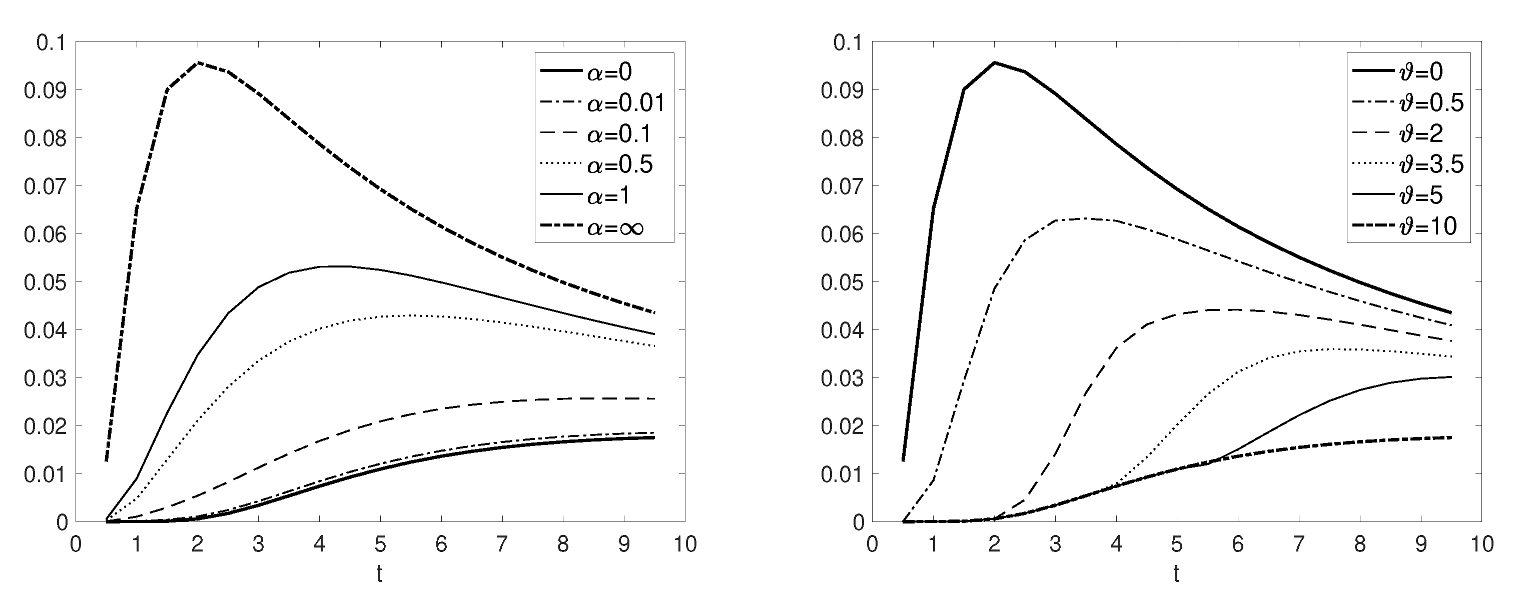
Some graphs of the probability of default for the GBM process are shown in Figure 3. We can observe that the larger the α value, the greater the probability of default is. This makes sense because as α increases, the firm has to carry more risks by allowing the counterparty to penalize more for the firm’s value staying below the occupation level. Similarly, we can say that the smaller the ϑ value, the greater the probability of default is, as the firm is required to default immediately once the occupation time exceeds the grace period. The difference between the models is that default probability values under the hazard rate model are more flexible across all maturity times, but the occupation time model does not correct the short-time behaviour whose values overlap with that in the Black–Cox model with default barrier A ( t ) .

7. Implied Hazard Rate Function

A reduced-form model is a model where a default event is characterized by a hazard rate (ordinary) function λ ( t ) . The hazard rate function is defined so that λ ( t ) Δ t is the probability of defaulting between time t and t + Δ t conditional on no default until time t (where τ is a default time):
λ ( t ) : = lim Δ t 0 P ˜ ( t τ t + Δ t τ > t ) Δ t = d d t P ˜ ( τ > t ) P ˜ ( τ > t ) .
If τ is the default time pre-specified by a model, then the hazard rate function implied by the model, denoted by λ * ( t ) , can be calculated using (59). Implied hazard rate functions provide a uniform way of comparing default behaviours across different models. Under the hazard rate model (with λ defined in (45)), the implied hazard rate function can be computed analytically via the spectral expansion method (assuming that the series in (57) can be differentiated term-by-term):14
λ * ( t ) = n = 1 λ ˜ n e λ ˜ n t a b m ( y ) ϕ ˜ n , α , ( x ) ϕ ˜ n , α , ( y ) d y n = 1 e λ ˜ n t a b m ( y ) ϕ ˜ n , α , ( x ) ϕ ˜ n , α , ( y ) d y .
Some graphs of the implied hazard rate functions are given in Figure 4. We can see that the implied hazard rate functions are generally increasing in time. For large α (small ϑ ), implied hazard rate functions increase sharply up to certain times, and decrease gradually (and end up converging to a certain value). The hazard rate functions under the occupation time model are relatively lower (especially for short times) compared to that under the hazard rate model. This observation makes sense from the shape of the probability of defaults described in Section 6.

8. Credit Default Swap (CDS) Spreads

We assume that there are p regular (time-proportional) payments on the time grid { T 1 , T 2 , , T p } with 0 < T 1 < < T p = T until the default event and one last payment at time τ . The fair price of the CDS spread is given by
R ( 0 , T ) : = D L ( 0 , T ) P L ( 0 , T ) = L G D [ e r f T P ˜ ( τ T ) + 0 T r f e r f u P ˜ ( τ u ) d u ] 0 T e r f u P ˜ ( τ > u ) d u 0 T r f e r f u ( u T β ( u ) 1 ) P ˜ ( τ > u ) d u .
where L G D [ 0 , 1 ] is the Loss Given Default, which is assumed to be deterministic, and β ( t ) { 1 , , p } is the index of the next payment date satisfying T β ( t ) 1 t < T β ( t ) . For our convenience, we shall rewrite the Equation (61) in terms of the survival probabilities:
R ( 0 , T ) = 1 e r f T P ˜ ( τ > T ) r f f ( T ) f ( T ) r f ( g ( T ) [ T p 1 f ( T ) i = 1 p ( T i T i 1 ) f ( T i ) ] )
where
f ( t ) : = 0 t e r f u P ˜ ( τ > u ) d u , g ( t ) : = 0 t u e r f u P ˜ ( τ > u ) d u .
We use the following proposition to calculate the fair value of the CDS spreads under the hazard rate model.
Proposition 1.
Under the hazard rate model (with λ defined in (45)), the time-0 value of a CDS spread is given in (62), where f and g are defined in (63), admit spectral expansion forms:15,16
f ( t ) = a b G ˜ α , ( r f ; x , y ) d y n = 1 e ( λ ˜ n + r f ) t λ ˜ n + r f a b m ( y ) ϕ ˜ n , α , ( x ) ϕ ˜ n , α , ( y ) d y , g ( t ) = a b λ G ˜ α , ( λ ; x , y ) d y λ = r f n = 1 1 + ( λ ˜ n + r f ) t ( λ ˜ n + r f ) 2 e ( λ ˜ n + r f ) t a b m ( y ) ϕ ˜ n , α , ( x ) ϕ ˜ n , α , ( y ) d y ,
where G ˜ , is the Green function defined by G ˜ α , ( λ ; x , y ) : = L t { p ˜ α , ( t ; x , y ) } ( λ ) .
Proof. 
For f , we can integrate term by term to obtain
f ( t ) = a b m ( y ) n = 1 ϕ ˜ n , α , ( x ) ϕ ˜ n , α , ( y ) λ ˜ n + r f n = 1 e ( λ ˜ n + r f ) t λ ˜ n + r f ϕ ˜ n , α , ( x ) ϕ ˜ n , α , ( y ) d y .
We know, by definition, that the first series in (65) is simply the Green function
G ˜ α , ( λ ; x , y ) = m ( y ) n = 1 ϕ ˜ n , α , ( x ) ϕ ˜ n , α , ( y ) λ ˜ n + λ .
For g we can employ the integration by parts formula to get
g ( t ) = n = 1 1 ( λ ˜ n + r f ) 2 1 + ( λ ˜ n + r f ) t ( λ ˜ n + r f ) 2 e ( λ ˜ n + r f ) t a b m ( y ) ϕ ˜ n , α , ( x ) ϕ ˜ n , α , ± ( y ) d y ,
where the first series in (67) can be expressed in terms of the Green function, and hence we obtain (64). □
Both series in (64) converge rapidly since the denominator λ ˜ n + r f tends to ∞ as n .

9. Calibration of CDS Spreads: GBM Case

We calibrate our models to some market data where the underlying firm’s value is assumed to be GBM. We extract the market CDS spreads data for the Total Energies company (TTE) with spot time on 1 June 2022. The market data contain eight sample market data points at the following tenor values: T = 0.5 , 1 , 2 , 3 , 4 , 5 , 7 , 10 years. Our calibration approach is find optimal parameter values that (locally) minimizes the gap between the market and model prices through a loss function. Here, we use the (unweighted) root mean squared error (RMSE) as the loss function (where Θ is the set of parameters in a given model):
L ( Θ ) = i = 1 8 R T i M d l R T i M k t 2 8
where R T i M k t is the i t h observed market CDS spread and R T i M d l is the CDS spread implied by the model at T i . We compare the following four models:
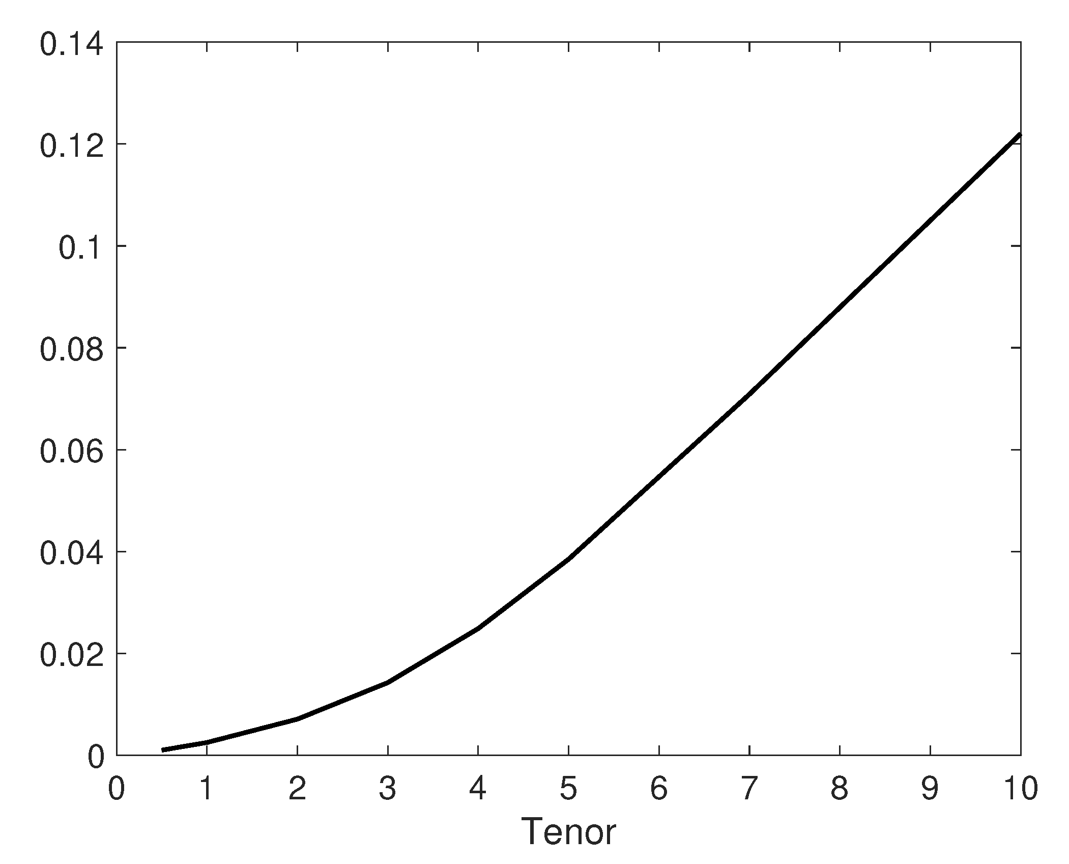
The summary of the market data used, as well as the calibration results, can be found in Table 1, Table 2 and Table 3. We employ an iterative scheme for our calibration procedure, that is, we calibrate parameters in the Black–Cox model, and then use the calibrated values as initial guesses to calibrate other parameters in the occupation time and hazard rate models. We do not use the iterative scheme for the Alfonsi–Lelong model since that model does not contain the default barrier A ( t ) . Figure 5 shows that the Black–Cox and occupation time models fitted poorly for small tenors. The hazard rate model significantly improve the result and led to a near-perfect calibration. The Alfonsi–Lelong model still outperforms the Black–Cox model, but is not as accurate as the hazard rate model. We use calibrated values from Table 3 to calculate the risk-neutral probabilities implied from the market CDS spreads under the hazard rate model. Based on Figure 6, we see that the Total Energies company is currently at a low default risk.

10. Conclusions

This study led to the innovation of two new credit risk models, namely, the occupation time and hazard rate models. They captured both Chapters 7 and 11 type defaults (the occupation time model was considered in Makarov et al. (2015); Makarov (2016) but the papers did not use the spectral expansion method). We derived closed-form pricing formulas for credit derivatives. Moreover, the hazard rate model prices can be expressed explicitly for diffusions, such as a geometric Brownian motion, and many other solvable processes. The pricing formulas under the occupation time model can be obtained by a Laplace inverse transformation of the hazard rate model. The Laplace inversion is performed numerically using the Gaver–Stehfest algorithm. The hazard rate model can capture versatile default probability values, which, in the occupation time models, are immovable at short maturity times. Our models are calibrated to the market CDS spreads from the Total Energies company. Our calibration results show that the computations are fast and lead to near-perfect calibrations to typical market CDS spread data.
Our main future work is to employ explicit expressions for alternative solvable diffusions. We can then consider pricing credit derivatives under such alternative models including the Constant Elasticity of Variance (CEV) model and other nonlinear local volatility models. Additionally, we can construct new structural models of credit risk based on the last passage time. In this paper, we have only considered senior debts, but we may also look into junior (subordinated) debts as well. One example is a contingent convertible (CoCo) bond which is a bond that converts into equity once the debt-to-equity ratio falls to a certain threshold level. CoCo bonds are popular among firms since firms can avoid default events, to a certain extent, by converting the CoCo bonds into equity once a catastrophic event triggers. We may also consider the pricing and calibrations of the new models to standard equity options, and thereby study the interplay between equity and credit markets.

Author Contributions

Conceptualization, G.C. and R.N.M.; methodology, G.C. and H.K.; software, G.C., H.K. and R.N.M.; validation, H.K.; formal analysis, G.C.; investigation, G.C., H.K. and R.N.M.; resources, H.K.; data curation, H.K.; writing—original draft preparation, H.K.; writing—review and editing, G.C. and R.N.M.; visualization, H.K.; supervision, G.C. and R.N.M.; project administration, G.C.; funding acquisition, G.C. and R.N.M. All authors have read and agreed to the published version of the manuscript.

Funding

This research was funded by the Natural Sciences and Engineering Research Council of Canada (NSERC) discovery grant numbers 2020-04782 and 2018-06176.

Institutional Review Board Statement

Not applicable.

Informed Consent Statement

Not applicable.

Data Availability Statement

Not applicable.

Conflicts of Interest

The authors declare no conflict of interest.

Appendix A. Explicit Expressions for a Drifted Brownian Motion

We provide explicit expressions on default probabilities and the CDS spread valuations for a Brownian motion with drift μ R , starting at x ( a , b ) with imposed killings at levels a, b where a < x < b .

Appendix A.1. Default Probabilities

In what follows, we provide explicit formulas for the integral in (57). Let { λ ˜ n } be the eigenvalues (refer to Equation (10)), satisfying the following eigenvalue equation:17
2 ( λ ˜ n α ) cos 2 ( λ ˜ n α ) ( a ) sin 2 λ ˜ n ( b ) + 2 λ ˜ n cos 2 λ ˜ n ( b ) sin 2 ( λ ˜ n α ) ( a ) = 0 , λ ˜ n > α , 2 ( α λ ˜ n ) sin 2 λ ˜ n ( b ) cosh 2 ( α λ ˜ n ) ( a ) + 2 λ ˜ n cos ( 2 λ ˜ n ( b ) ) sinh 2 ( α λ ˜ n ) ( a ) = 0 , λ ˜ n ( 0 , α ) ,
and let { ϕ ˜ n , α , } be the eigenfunctions given as follows. We only provide formulas for x (i.e., the firm’s value starts above the liquidation level) since the other case is rarely used in practice.
  • If x [ , b ) , y ( a , ] , λ ˜ n ( 0 , α ) ,
    ϕ ˜ n , α , ( x ) ϕ ˜ n , α , ( y ) = sin ( 2 λ ˜ n ( b ) ) ( b a ) sinh ( 2 ( α λ ˜ n ) ( a ) + cosh ( 2 ( α λ ˜ n ) ( a ) ) 2 ( α λ ˜ n ) cos ( 2 λ ˜ n ( b ) ) sinh ( 2 ( α λ ˜ n ) ( a ) ) 2 λ ˜ n + α λ ˜ n λ ˜ n ( b ) λ ˜ n α λ ˜ n ( a ) cosh ( 2 ( α λ ˜ n ) ( a ) ) 1 × sin ( 2 λ ˜ n ( b x ) ) sinh ( 2 ( α λ ˜ n ) ( y a ) ) .
  • If x [ , b ) , y ( a , ] , λ ˜ n > α ,
    ϕ ˜ n , α , ( x ) ϕ ˜ n , α , ( y ) = sin ( 2 λ ˜ n ( b ) ) ( b a ) sin ( 2 ( λ ˜ n α ) ( a ) cos ( 2 ( λ ˜ n α ) ( a ) ) 2 ( λ ˜ n α ) cos ( 2 λ ˜ n ( b ) ) sin ( 2 ( λ ˜ n α ) ( a ) ) 2 λ ˜ n + λ ˜ n α λ ˜ n ( b ) + λ ˜ n λ ˜ n α ( a ) cos ( 2 ( λ ˜ n α ) ( a ) ) 1 × sin ( 2 λ ˜ n ( b x ) ) sin ( 2 ( λ ˜ n α ) ( y a ) ) .
  • If x [ , b ) , y [ , b ) , λ ˜ n ( 0 , α ) ,
    ϕ ˜ n , α , ( x ) ϕ ˜ n , α , ( y ) = 2 ( α λ ˜ n ) cosh ( 2 ( α λ ˜ n ) ( a ) ) sin ( 2 λ ˜ ( a ) ) 2 λ ˜ n cos ( 2 λ ˜ n ( a ) ) sinh ( 2 ( α λ ˜ n ) ( a ) 2 λ ˜ n sin ( 2 λ ˜ n ( b a ) ) × cos ( 2 λ ˜ n ( b ) ) sinh ( 2 ( α λ ˜ n ) ( a ) ) 2 λ ˜ n + α λ ˜ n λ ˜ n ( b ) λ ˜ n α λ ˜ n ( a ) cosh ( 2 ( α λ ˜ n ) ( a ) ) sin ( 2 λ ˜ n ( b ) ) ( b a ) sinh ( 2 ( α λ ˜ n ) ( a ) + cosh ( 2 ( α λ ˜ n ) ( a ) ) 2 ( α λ ˜ n ) 1 × sin ( 2 λ ˜ n ( b x ) ) sin ( 2 λ ˜ n ( b y ) ) .
  • If x [ , b ) , y [ , b ) , λ ˜ n > α ,
    ϕ ˜ n , α , ( x ) ϕ ˜ n , α , ( y ) = 2 ( λ ˜ n α ) cos ( 2 ( λ ˜ n α ) ( a ) ) sin ( 2 λ ˜ ( a ) ) 2 λ ˜ n cos ( 2 λ ˜ n ( a ) ) sin ( 2 ( λ ˜ n α ) ( a ) 2 λ ˜ n sin ( 2 λ ˜ n ( b a ) ) × cos ( 2 λ ˜ n ( b ) ) sin ( 2 ( λ ˜ n α ) ( a ) ) 2 λ ˜ n + λ ˜ n α λ ˜ n ( b ) + λ ˜ n λ ˜ n α ( a ) cos ( 2 ( λ ˜ n α ) ( a ) ) sin ( 2 λ ˜ n ( b ) ) ( b a ) sin ( 2 ( λ ˜ n α ) ( a ) cos ( 2 ( λ ˜ n α ) ( a ) ) 2 ( λ ˜ n α ) 1 × sin ( 2 λ ˜ n ( b x ) ) sin ( 2 λ ˜ n ( b y ) ) .
Then, by the Girsanov theorem (or via a Doob h-transform), the transition density of the drifted Brownian motion follows as
p ˜ ( a , b ) , α , ( T ; x , y ) = e μ ( y x ) μ 2 T 2 n = 1 2 e λ ˜ n T ϕ ˜ n , α , ( x ) ϕ ˜ n , α , ( y ) ,
where ϕ ˜ n , α , ( x ) ϕ ˜ n , α , ( y ) is given by (A2)–(A5). To implement (57), the integrals
a b e μ ( y x ) ϕ ˜ n , α , ( x ) ϕ ˜ n , α , ( y ) d y , n 1
can be obtained explicitly by direct computations.

Appendix A.2. CDS Spread

Let { λ ˜ n } be the eigenvalues and let { ϕ ˜ n , α , } be the eigenfunctions defined in (A1)–(A5). Then we have explicit formulas for f and g , defined in Proposition 1:
f ( t ) = a b e μ ( y x ) G ˜ α , ( r f + μ 2 / 2 ; x , y ) d y n = 1 e ( λ ˜ n + r f + μ 2 / 2 ) t λ ˜ n + r + μ 2 / 2 a b 2 e μ ( y x ) ϕ ˜ n , α , ( x ) ϕ ˜ n , α , ( y ) d y , g ( t ) = a b e μ ( y x ) λ G ˜ α , ( λ ; x , y ) d y λ = r f + μ 2 / 2 n = 1 1 + ( λ ˜ n + r f + μ 2 / 2 ) t ( λ ˜ n + r f + μ 2 / 2 ) 2 e ( λ ˜ n + r f + μ 2 / 2 ) t a b 2 e μ ( y x ) ϕ ˜ n , α , ( x ) ϕ ˜ n , α , ( y ) d y ,
where G ˜ α , ( λ ; x , y ) is the Green function with explicit expressions given below (we only provide for x ):
  • If y ( a , ] ,
    G ˜ ( a , b ) , α , ( λ ; x , y ) = 2 sinh ( 2 λ ( b x ) ) sinh ( 2 λ + 2 α ( y a ) ) 2 λ cosh ( 2 λ ( b ) ) sinh ( 2 λ + 2 α ( a ) ) + 2 λ + 2 α cosh ( 2 λ + 2 α ( a ) ) sinh ( 2 λ ( b ) ) ,
  • If y [ , b ) ,
    G ˜ ( a , b ) , α , ( λ ; x , y ) = 2 sinh ( 2 λ ( x y a ) ) sinh ( 2 λ ( b x y ) ) 2 λ sinh ( 2 λ ( b a ) ) + 2 sinh ( 2 λ ( b x ) ) sinh ( 2 λ ( b y ) ) 2 λ sinh ( 2 λ ( b a ) ) × 2 λ cosh ( 2 λ ( a ) ) sinh ( 2 λ + 2 α ( a ) ) 2 λ + 2 α cosh ( 2 λ + 2 α ( a ) ) sinh ( 2 λ ( a ) ) 2 λ cosh ( 2 λ ( b ) ) sinh ( 2 λ + 2 α ( a ) ) + 2 λ + 2 α cosh ( 2 λ + 2 α ( a ) ) sinh ( 2 λ ( b ) ) ,
and the integral
a b e μ ( y x ) G ˜ α , ( λ ; x , y ) d y
can be obtained explicitly as well. In practice, due to the lengthy expressions of the Green function, we may obtain
a b e μ ( y x ) λ G ˜ α , ( λ ; x , y ) d y = λ a b e μ ( y x ) G ˜ α , ( λ ; x , y ) d y
by numerical differentiations (since it is a smooth function in λ ).

Notes

1
Here we distinguish the X-diffusion from the F-diffusion (i.e., the firm’s value process) F : = F ( X ) which is obtained through a smooth monotonic mapping F : I D (where D is the state space for the F-diffusion) with unique inverse X = F 1 .
2
The cemetery state is not included in the interval I . When the process is killed and immediately sent to the cemetery state, it stays there indefinitely.
3
E x [ X ; A ] : = E x [ X I A ] for any random variable X and event A.
4
P x X ˜ ( a , b ) , t d y : = P X ˜ ( a , b ) , t d y X 0 = x .
5
When α = 0 , we obtain the regular transition density of X ( a , b ) without an instantaneous killing:
p ( a , b ) ( t ; x , y ) d y : = P x X t d y , m t > a , M t < b ; t > 0 , x , y ( a , b ) ,
and zero otherwise.
6
The transition and joint densities are pointwise convergent as b r :
p ˜ ( a , r ) , α , ( t ; x , y ) : = lim b r p ˜ ( a , b ) , α , ( t ; x , y ) , f A t , , X t ( a , r ) ( u , y x ) : = lim b r f A t , , X t ( a , b ) ( u , y x ) .
7
We assume there exists a risk-neutral probability P ˜ equivalent to P so that the discounted price process of the defaultable claim is a Doob–Levy ( P ˜ , F ) -martingale. In the GBM model, we clearly have the discounted firm’s value process e r f t F t = F 0 e σ 2 2 t + σ W ˜ t , t 0 , as a ( P ˜ , F ) -martingale.
8
E ˜ t , A , x h ( τ T , X ˜ τ T ) : = E ˜ h ( τ T , X ˜ τ T ) A t , = A , X t = x .
9
For 0 t < T , Theorem 1 extends to the time-t value of the credit derivative since D t , A , x ϑ , T = D 0 , x ϑ A , T t , thanks to Lemma 1.
10
τ ( ϑ ) T = τ a T ( a . s . ) , for ϑ T , where the T-maturity credit derivative price D 0 , x ϑ , T corresponds to that in the Black–Cox model with default barrier A ( t ) .
11
The name “hazard rate model” comes from the fact that we are employing a hazard rate process to model default probabilities.
12
For 0 t < T , Theorem 2 extends to the time-t value of the credit derivative: D t , x α , T = D 0 , x α , T t .
13
We can easily extend it to the hazard rate model with λ defined in (48), since
P ˜ x ( τ ( α 1 , α 2 ) > T ) = e α 1 T a p ˜ ( a , ) , α 2 α 1 , ( T ; x , y ) .
14
Under the occupation time model, the implied hazard rate function can be computed by Laplace inverting, with respect to α , of the numerator and denominator in (60) separately.
15
We can easily extend it to the hazard rate model with λ defined in (48), by sending r f r f + α 1 and α α 2 α 1 .
16
Under the occupation time model, the implied hazard rate function can be computed by Laplace inverting, with respect to α , of f and g in (64).
17
The eigenvalues { λ ˜ n } n 1 can be obtained numerically by the bisection or Newton-Raphson methods.

References

  1. Alfonsi, Aurélien, and Jérôme Lelong. 2012. A closed-form extension to the Black-Cox model. International Journal of Theoretical and Applied Finance 15: 1250053. [Google Scholar] [CrossRef] [Green Version]
  2. Bielecki, Tomasz R., and Marek Rutkowski. 2013. Credit Risk: Modeling, Valuation and Hedging. Berlin/Heidelberg: Springer. [Google Scholar]
  3. Black, Fischer, and John C. Cox. 1976. Valuing corporate securities: Some effects of bond indenture provisions. The Journal of Finance 31: 351–67. [Google Scholar] [CrossRef]
  4. Borodin, Andrei N., and Paavo Salminen. 2002. Handbook of Brownian Motion—Facts and Formulae, 2nd ed. Probability and Its Applications. Basel: Birkhäuser. [Google Scholar]
  5. Broadie, Mark, Mikhail Chernov, and Suresh Sundaresan. 2007. Optimal debt and equity values in the presence of Chapter 7 and Chapter 11. Journal of Finance 62: 1341–77. [Google Scholar] [CrossRef]
  6. Campolieti, Giuseppe. Solvable Diffusions in Financial Mathematics. manuscript in preparation, to be published.
  7. Campolieti, Giuseppe, Roman N. Makarov, and Karl Wouterloot. 2013. Pricing step options under the CEV and other solvable diffusion models. International Journal of Theoretical and Applied Finance 16: 1350027. [Google Scholar] [CrossRef] [Green Version]
  8. Chesney, Marc, Monique Jeanblanc-Picqué, and Marc Yor. 1997. Brownian excursions and Parisian barrier options. Advances in Applied Probability 29: 165–84. [Google Scholar] [CrossRef]
  9. Cohen, Alan M. 2007. Numerical Methods for Laplace Transform Inversion. New York: Springer, vol. 5. [Google Scholar]
  10. Galai, Dan, Alon Raviv, and Zvi Wiener. 2007. Liquidation triggers and the valuation of equity and debt. Journal of Banking and Finance 31: 3604–20. [Google Scholar] [CrossRef]
  11. Gaver, Donald P., Jr. 1966. Observing stochastic processes, and approximate transform inversion. Operations Research 14: 444–59. [Google Scholar] [CrossRef]
  12. Haber, Richard J., Phillip J. Schönbucher, and Paul Wilmott. 1999. Pricing Parisan Options. The Journal of Derivatives 6: 71–79. [Google Scholar] [CrossRef]
  13. Li, Bin, Qihe Tang, Lihe Wang, and Xiaowen Zhou. 2014. Liquidation risk in the presence of Chapters 7 and 11 of the US bankruptcy code. Journal of Financial Engineering 1: 1450023. [Google Scholar] [CrossRef] [Green Version]
  14. Linetsky, Vadim. 2004. The spectral decomposition of the option value. International Journal of Theoretical and Applied Finance 7: 337–84. [Google Scholar] [CrossRef]
  15. Makarov, Roman N., Adam Metzler, and Zi Ni. 2015. Modelling default risk with occupation times. Finance Research Letters 13: 54–65. [Google Scholar] [CrossRef]
  16. Makarov, Roman N. 2016. Modeling liquidation risk with occupation times. International Journal of Financial Engineering 3: 1650028. [Google Scholar] [CrossRef]
  17. Merton, Robert C. 1974. On the pricing of corporate debt: The risk structure of interest rates. The Journal of finance 29: 449–70. [Google Scholar]
  18. Moraux, Franck. 2002. Valuing Corporate Liabilities When the Default Threshold Is Not an Absorbing Barrier. Available online: https://www.worldscientific.com/doi/10.1142/9789814759595_0014 (accessed on 12 December 2021).
  19. Nardon, Martina. 2008. First passage and excursion time models for valuing defaultable bonds: A review with some insights. Frontiers in Finance and Economics 5: 1–25. [Google Scholar]
  20. Stehfest, Harald. 1970. Algorithm 368: Numerical inversion of Laplace transforms. Communications of the ACM 13: 47–49. [Google Scholar] [CrossRef]
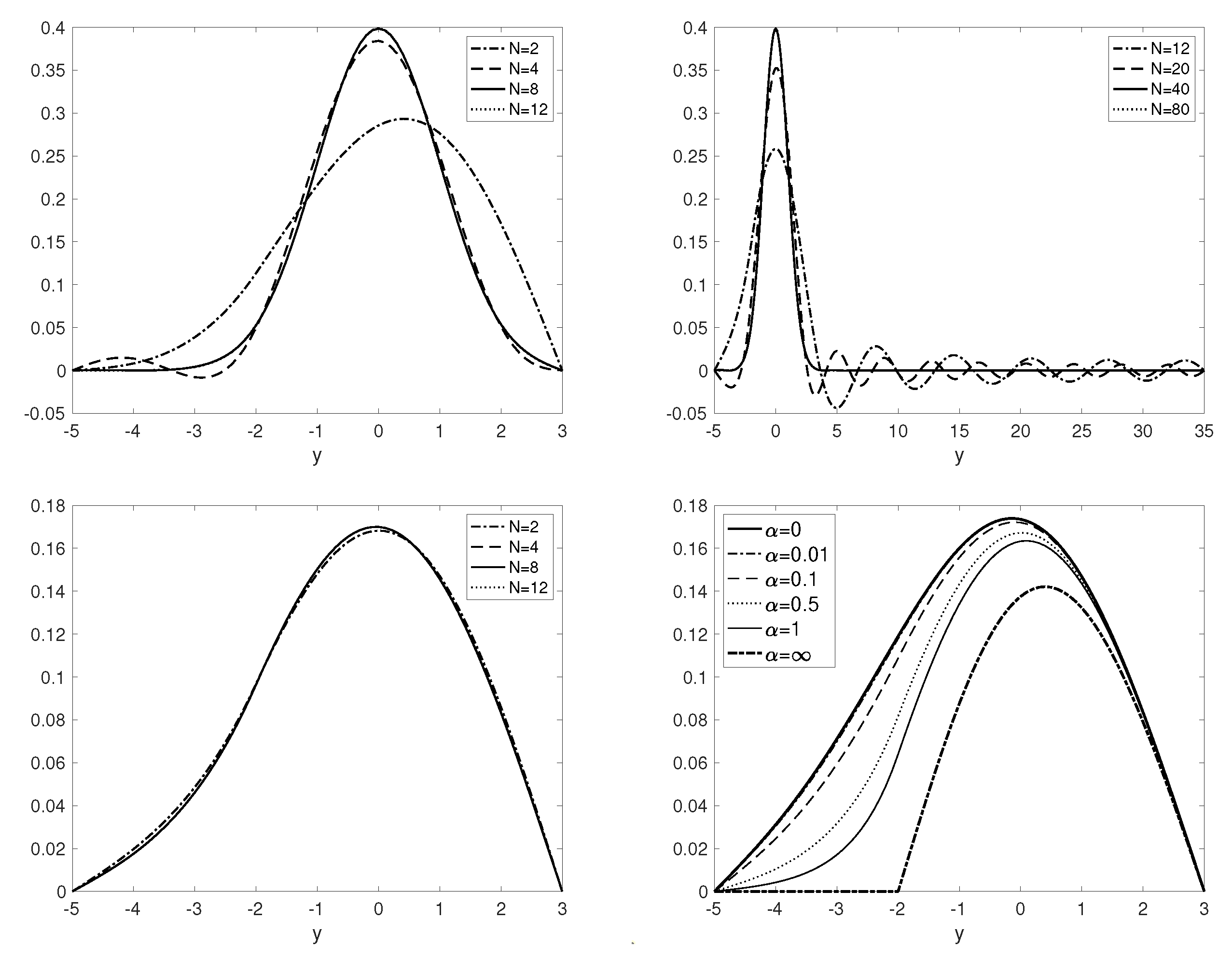
Figure 1. Graphs of the transition density in (9) where X = W is a standard Brownian motion with a = −5, b = 3 (b = 35 for top-right), = −2, t = 1 (top-left, bottom-left) t = 5 (top-right, bottom-right), α = 0.25 (except bottom-right), N = 30 (bottom-right).
Risks 10 00228 g001
Figure 2. Graphs of the joint density in (11) where X = W is a standard Brownian motion with a = −5, b = 3, = −2, t = 5, and N = 30. We used 16 terms in the Gaver–Stehfest algorithm.
Risks 10 00228 g002
Figure 3. Graphs of default probabilities for the hazard rate (left) and occupation time models (right). The underlying firm’s value is GBM with F 0 = 100 , L 0 = 50 , A 0 = 20 , r f = 5 % , σ = 30 % , γ = 5 % , and N = 30 . For the right graph, we used 16 terms in the Gaver–Stehfest algorithm.
Risks 10 00228 g003
Figure 4. Graphs of implied hazard rate functions for the hazard rate model (left) and occupation time model (right). The underlying firm’s value is GBM with F 0 = 100 , L 0 = 50 , A 0 = 20 , r f = 5 % , σ = 30 % , γ = 5 % , and N = 30 . For the right graph, we used 16 terms in the Gaver–Stehfest algorithm.
Risks 10 00228 g004
Figure 5. Graphs of CDS Spreads for four models: Black–Cox (top-left), occupation time (top-right), Alfonsi–Lelong (bottom-left), and hazard rate (bottom-right). The underlying firm’s value is GBM.
Risks 10 00228 g005
Figure 6. Implied risk-neutral probability for the hazard rate model (the underlying firm’s value is GBM).
Risks 10 00228 g006
Table 1. Initial Information about the market.
Variable NameDescriptionValue
F 0 initial firm’s value 55.59
r f constant risk-free rate 5 %
σ constant volatility 28 %
L G D constant Loss Given Default 0.6
Table 2. Market Data of Tenor (year) and CDS spread (bps).
Tenor0.512345710
CDS11.8615.1321.2928.7937.2145.8360.0373.17
Table 3. Calibration Results for model parameters (the underlying process is GBM). NA means not applicable.
VariableDescriptionBlack–CoxOccupationA–LHazard Rate
A 0 default barrier (at time 0) 18.96 13.47 NA 12.83
γ growth rate of barrier 3.51 % 0.19 % 11.22% 0.32 %
L 0 occupation barrier (at time 0)NA23.2928.7838.42
θ / T grace period relative to TNA0.2368NANA
α 1 killing rate (above L)NANA0.27% 0.18 %
α 2 killing rate (below L)NANA3.42% 2.33 %
loss function value 5.70 × 10 6 5.16 × 10 6 3.10 × 10 8 5.77 × 10 10
Publisher’s Note: MDPI stays neutral with regard to jurisdictional claims in published maps and institutional affiliations.