1. Introduction
Within the nature of the insurance business, and well-documented, for instance, by
Wüthrich and Merz (
2008) or by
Farny (
2011), the determination of claims reserves is related to uncertainty. Models are used to reflect complex circumstances. Parameters are estimated, resulting in parameter risks. Unpredictable loss occurrence is observed and caused, for instance, by random fluctuations. Changes in the claims handling process or legislative amendments bear further unexpected uncertainties. Safety considerations finally join the reason to build up equalization reserves for reinsurance and non-life undertakings, requested by the Swiss Financial Market Supervisory Authority—
FINMA (
2008a, rank no. 8;
2011, rank no. 37). For example, a natural catastrophe (CAT) has a low probability of occurrence, and by occurring, CAT causes a high loss. In good financial times, the insurance undertaking put aside the equalization reserve to dampen the future loss burden, see
Dacorogna et al. (
2013). These authors explain how even shareholders benefit from the equalization reserves.
1.1. Equalization Reserves in Other Countries
Hindley (
2017) defines “equalization reserve” in the UK as an amount to smooth the reserves over time, typically considering low frequency/high severity events.
Akhurst et al. (
1992) point out the philosophical viewpoint of holding either a specific reserve or a surplus solvency fund after tax to finance a future large claim. Furthermore, non-technical elements such as investment and management costs could require a kind of equalization reserve in some countries, see
Akhurst et al. (
1992). These authors present the calculation and the handling of the equalization reserves for the UK, Denmark, Finland, France, Germany, Italy, The Netherlands, Norway, Spain and Sweden.
1.2. Swiss Insurance Supervision
In order to protect creditors, investors and policyholders, FINMA supervises, among others, private insurance companies, complying with the Insurance Supervision Act (ISA)
1 and with the Ordinance on the Supervision of Private Insurance Companies (ISO)
2. FINMA has regulatory power and regulates using ordinances and circulars as stated in the core tasks, see
FINMA (
2019b). FINMA’s predecessor was the Federal Office of Private Insurance (FOPI), being responsible until 2008. In Switzerland, reinsurance and non-life undertakings are obliged to hold equalization reserves within their statutory accounts, regardless of whether these entities cover low frequency/high severity events. The handling of the equalization reserves has to be described in the technical part of the business plan of an undertaking. Appendix C of ISO-
FINMA (
2015) does not explicitly list the equalization reserves to be disclosed.
The reserves of the Swiss capital model (SST) are based on the best estimate principle, as stated by
FINMA (
2017): the insurance liability includes all future financial expenditures to fulfill those liabilities, excluding the capital costs. As a consequence, the equalization reserves are set to zero. Target capital is the calculated capital to meet the quantitative requirements under the SST, see
FINMA (
2018a). The target capital has to be covered by own funds. Insurance/reserving risk is part of this target capital. In the case in which the actual case reserves would not be sufficient, the shareholder’s own fund would fill this gap. Due to safety considerations, the SST requests for insurance/reserving risk and the statutory accounts request for equalization reserves. However, within SST, the insurance/reserving risk is covered by own funds, and within the statutory accounts, the equalization reserves are insurance liabilities.
Due to solvency requirements, the focus of the recent actuarial studies lay on market-consistent valuation of the balance sheet.
Wüthrich (
2016) presents market-consistent actuarial valuation of the insurance reserves. In the literature the classical claims reserving methods are well studied, see
Wüthrich and Merz (
2008). On the other hand, the calculation or the handling of the statutory required equalization reserves are not explicitly covered. FINMA’s circulars clarify the legal requirements.
1.3. Literature Review
The Swiss Association of Actuaries,
SAV (
2006), publishes guidelines for loss reserves in non-life insurance, focusing on required reserves for claims handling costs. However, the equalization reserves are not mentioned. FINMA’s circulars define the legal scope to handle this kind of reserve for reinsurance and for non-life undertakings.
Hindley (
2017) discusses the equalization reserves in the UK.
Akhurst et al. (
1992) present equalization reserves modeling in UK, Denmark, Finland, France, Germany, Italy, The Netherlands, Norway, Spain and Sweden.
De Vylder and Goovaerts (
1999) present a theoretical evaluation of the equalization reserves. A broad literature regarding Swiss equalization reserves does not exist. This article steps forward to fill the gap.
1.4. Present Research
We start defining “equalization reserves” separately for reinsurance and for non-life undertakings. Thereafter, we look at the handling of the equalization reserves within International Financial Reporting Standards 17 (IFRS 17) and within the capital modeling. As tax consideration impacts the insurance undertakings, we look closer at the mechanism from an actuarial point of view. We do not know how the undertakings calculate the equalization reserve. FOPI and FINMA implicitly disclose the equalization reserves. Therefore, we describe our method to estimate the equalization reserves from the reported statutory accounts and we apply a model to detect the relationship between the equalization reserves and the statutory accounts items.
This paper is structured as follows: in
Section 2, we define equalization reserves and we look closer at accounting and capital model aspects. Hereafter, in
Section 3, we formalize the model and based on this, we consider taxes. Further, in
Section 4, we concretize the formalism on the publicly available data, we present the general approach of the generalized additive model (GAM), the generalized linear model (GLM) and the model results. Finally, in
Section 5, we discuss the results and in
Section 6 we conclude.
2. Definition, Accounting and Capital Model Aspects
In Switzerland, equalization reserves are defined separately for reinsurance and for non-life undertakings. In principle, these definitions are the same for both types of undertakings. However, there are small differences, which we point out in the following. In
Section 2.1, we define equalization reserves for reinsurance and for non-life undertakings in Switzerland. Thereafter in
Section 2.2, we look at the handling of the equalization reserves within statutory accounting, within IFRS and within the Swiss capital modeling.
2.1. Definition
In Switzerland, the ISA distinguishes between legal entities, writing direct business, for instance, non-life undertakings, and legal entities only writing indirect business for reinsurance undertakings. Non-life undertakings control each single risk, by selecting the risk and by complying with the underwriting policy. In general, reinsurance undertakings protect the portfolio of undertakings, whereby the single risks could not be controlled. In consequence, the risk profiles of non-life undertakings and reinsurance undertakings are different and a separate analysis is appropriate. In this section, we define equalization reserves for reinsurance and for non-life undertakings in Switzerland.
2.1.1. Equalization Reserves for Reinsurance Undertakings
In Switzerland, the equalization reserves
3 for reinsurance undertakings are defined as the technical reserve, balancing unfavorable development and fluctuations of incurred claims, see
FINMA (
2011, rank no. 37). According to
FINMA (
2011, rank no. 8*) reinsurance undertaking could keep equalization reserves within the statutory accounts and are requested to specify methods and principles to establish and to dissolve equalization reserves within the business plan in accordance with Art. 4, section 2, letter d of ISA.
2.1.2. Equalization Reserves for Non-Life Undertakings
In Switzerland, the equalization reserves
4 for non-life undertakings are defined as the technical reserves, wholly or partially balancing unfavorable development and fluctuation of incurred claims, see
FINMA (
2008a, rank no. 8). In particular, the equalization reserves comprise:
The reserves covering parameter risk, safety considerations and unpredictable loss fluctuation according to
FINMA (
2008a, rank no. 16);
Equalization reserves for the credit insurance business, see
FINMA (
2008a, rank no. 18).
There is no general standard formula for the non-life undertakings to calculate the equalization reserves
5. Thus, each company determines its own method. According to Art. 69 of ISO, the equalization reserves are part of the total technical reserves of a non-life insurance undertaking.
FINMA (
2008a, rank no. 14 ff) requests the non-life undertaking to specify methods and principles to establish and to dissolve equalization reserves within the business plan in accordance with Art. 4, section 2, letter d of ISA.
2.2. Accounting and Capital Model Aspects
In this section, we look at the handling of the equalization reserves within statutory accounting, within IFRS and within the Swiss capital modeling.
2.2.1. Statutory Accounting
The required equalization reserves are technical reserves reported as a liability in the statutory balance sheet, see ISO-
FINMA (
2015). For non-life undertakings, according to Art. 71 of ISO, the equalization reserves are part of the amount covered by the tied assets. From the Swiss statutory accounting point of view, the equalization reserves belong to the policyholders. However, the equalization reserves cannot be uniquely assigned to a single customer. In the case of discontinuation of a company, the release of the equalization reserves could strengthen either the case reserves or the own capital, taking into account the tax requirements.
2.2.2. IFRS
Regarding IFRS 17, the best estimate of liabilities should be among others “current”, reflecting the most recent existing information, for instance, see
Dunne et al. (
2017). As a consequence, within IFRS 17, future catastrophe losses occurring outside the contract boundaries are not considered within the insurance liabilities. Nevertheless, within the Swiss statutory accounting, these catastrophe losses could be covered by the equalization reserves.
2.2.3. Capital Modeling
The SST assesses the capital solvency situation of an insurance undertaking, see
FINMA (
2018b). The valuation of the liability as “best estimate” for claims, incurring prior to the reference date of the balance sheet, is the basis for the risk-bearing capital-calculation according to
FINMA (
2017). As a consequence, equalization reserves are not considered in the SST balance sheet. The European Solvency II framework uses a similar approach to define the insurance liabilities: equalization reserves are excluded from the best estimate of liabilities, see
EIOPA (
2015). Thus, the handling of the equalization reserves within Solvency II and IFRS 17 is the same.
According to Art. 41 para. 3 of ISO, the market value margin (MVM) corresponds to the capital costs of the risk bearing capital. MVM has to be kept as an insurance liability in the SST balance sheet, see
FINMA (
2017, rank no. 51) and MVM intends to fulfill the insurance liabilities, see
FINMA (
2017, rank no. 52). Similar to MVM, Solvency II requires a risk margin, based on the one-year view. In IFRS 17, a margin is requested for risk adjustment, based on a lifetime view, to be taken into account within the technical provisions, see
England et al. (
2019). However, this discounted capital cost does not have the same purpose as the statutory equalization reserves: MVM’s purpose is to cover capital costs and the equalization reserves’ purpose is to balance unfavorable development and the fluctuation of incurred claims. Similarly, MVM and the equalization reserves intend to provide an additional safety cushion to develop incurred claims.
Within the SST standard-model for non-life undertakings, target capital consists, among others, of the insurance risk comprising reserving risk, normal, large and NatCat claims according to
FINMA (
2018a). The definitions are as follows:
Reserve risk: risk out of claims being greater than expected;
Normal claims: risk out of claims below a threshold—high frequencies/low severities;
Large claims: risk out of claims above a threshold—low frequencies/high severities;
Nat Cat: risk out of claims occurred due to natural catastrophe event.
SST’s insurance risk and the statutory equalization reserves have some features in common. However, SST’s insurance risk is part of the target capital, and the equalization reserves are statutory balance sheet liabilities.
Similar to SST’s insurance risk, Solvency II handles reserves risk, for which
England et al. (
2019) present analytic and simulation-based approaches. In the classical sense, the prediction error to quantify reserve risk consists, in general, of the uncertainty within the estimation of parameters and within the underlying claims generating process. This reserve risk heads in the same direction as the equalization reserves, balancing unfavorable development and fluctuation of incurred claims.
3. Preparation for the Model and Tax Considerations
This section starts with basic ideas to model equalization reserves. Thereafter, in
Section 3.2, we use the introduced formalism to develop tax considerations linked to these equalization reserves. While FOPI and FINMA implicitly published the equalization reserves as part of the technical reserves, we restate these equalization reserves by using FOPI’s and FINMA’s published figures. In
Section 3.3.1, we present the restatement for reinsurance undertakings, and in
Section 3.3.2, for non-life undertakings.
3.1. Basic Idea of the Model
We present a model to study the factors influencing the equalization reserves. We start looking at the modeling in Europe and thereafter, we develop our conceptual approach.
3.1.1. Modelling in Europe
Akhurst et al. (
1992) list two features to build up the equalization reserves: the upper limit of the equalization reserves and the transfer rule to build and to release reserves. They present four formulas to define the upper limit:
Short-term fluctuation, cycles, trends and potential risk cumulation;
Standard deviation of the claims;
A coefficient, depending on the line of business, multiplied by the premium income;
A combination out of premium income, variance and oversea risks.
Within Europe
Sandström (
2005) promotes further harmonization of the equalization reserves by linking the equalization reserves to the volatility of business. As transfer rules
Akhurst et al. (
1992) present:
Recognition of the underwriting result;
Deviation of the incurred claims ratio from the average level;
Deviation of the incurred claims ratio from a fixed constant level;
An asymmetric formula depending on the underwriting result;
An open and half-open transfer (not only depending on the underwriting results);
Other specific rules.
3.1.2. Conceptual Approach
In its business plan, each Swiss insurance undertaking defines the upper limit and the corresponding transfer rule to the equalization reserves. Both are unknown to us since they are not disclosed. Nevertheless, we propose to approximate a transfer rule to the equalization reserves with the help of the profit and loss items. We analyze the transfer rule based on the underwriting result: premium income, other income, insurance costs (payments and change in technical reserves) and administration costs. The classical approach to calculate the technical result (
TRe) of an undertaking is, according to
Farny (
2011), the sum of the income, premium (
Pre) and other income (
OIn), minus the costs, insurance cost (
ICo) and operation cost (
OCo):
Insurance cost (
OIn) consists of claims payments and changes (“Δ”) in total technical reserves. The equalization reserves (
ER) are part of the total technical reserves. Therefore, insurance cost is the sum of insurance cost without change in equalization reserves (
ICo_woΔER) plus change in equalization reserves (Δ
ER). Accordingly, we transform the insurance costs:
The actual equalization reserves (
ER) are the sum out of the change in equalization reserves (Δ
ER) and the equalization reserves of the prior year (
ER_PY):
Using (
2) we transform (
1) into:
which yields for (
3):
The size of the equalization reserves depends on the profit and loss items and on their previous year’s amount.
In addition to the above, we are interested in the potential influence of the accounting year, of the company age and of the legal form. In
Section 4, we use FOPI’s and FINMA’s published net data to analyze the impact of these items.
Equation (
5) could take outward reinsurance into account. The equalization reserves have to cover the whole gross business on the one hand. On the other hand, the net business reflects the remaining risk exposure to be covered. An undertaking does not transfer parts of the equalization reserves to the reinsurer and independently, the reinsurer estimates the equalization reserves on its own portfolio. As net data are available, we analyze the numbers net of reinsurance.
3.2. Tax Considerations
To quote the words from Benjamin Franklin, “Nothing is certain but death and taxes”. Therefore, we consider tax in connection with equalization reserves.
Change in the equalization reserves impacts the net profit of the fiscal year and herewith the taxable amount. Therefore, we take a closer look at the taxation and the net profit of insurance companies. An insurance undertaking’s net profit consists of a non-technical and technical part. We are only interested in the technical one (
TRe). The taxation rate (
Tax) could change over the years. To keep the system simple, we assume a constant taxation rate over time (
t). Adding the time reference (
) to the items we obtain from (
1) in combination with (
2):
The change in equalization reserves reduces the taxable amount in the fiscal year
t. Let us assume
is the year in which a significant loss occurs of height
, triggering the equalization reserves and assuming
. Thus, the equalization reserves of the prior year are dissolved completely (
). The taxable amount of (
6) is transformed to:
Due to the assumption
we know that
Furthermore, we assume that the income does not cover the cost. This results in
The release of the equalization reserves reduces the loss of the technical result in the year
. This reduced loss may be offset by future profits over a period of seven years after the year
. Changes in equalization reserves reduce future profits. However, to benefit from loss-offsetting with future profits, a profit has to be reported. This conflict of interest is born within the loss-offsetting with future profits over a period of seven years and the conflict is solved by the written business plan: the rules to establish the equalization reserves define how much the undertaking has to build up the equalization reserves.
Table 1 illustrates this circumstance:
The Swiss tax regulation counteracts tax-optimization, using the equalization reserves: the scope of the business plan limits the establishment and the release of the equalization reserves. The loss-offsetting with future profit incentivizes an optimization-problem of profit shifting over time. Going concerns assumed, the equalization reserves belong to the insured, and some day, they will be taxed. From the pure actuarial point of view, tax-optimization is not taken into account to define rules to establish or release the equalization reserves, and by defining an upper bound for the equalization reserves. As equalization reserves may be easily misused for tax-optimization, governments looked at different possibilities to handle the valuation of equalization reserves.
Akhurst et al. (
1992) state that the taxation legislations “vary widely in different countries”. In some countries, the established equalization reserves should be released within a duration of, e.g., ten years.
3.3. Restatement of Equalization Reserves
By act of law Art. 25 of ISA, insurance undertakings report to FINMA the financial statements and the supervisory report, and FINMA publishes the annual financial statements
7,
8.
FOPI (
2007) disclosed the financial years 1997 to 2007 and since 2008 FINMA is in charge, see
FINMA (
2019a).
FOPI and FINMA have disclosed the figures in a different setup. In
Appendix A and
Appendix B, further details of the main changes and the source of the variables, which we use as explanatory ones, are provided. In
Section 4, we describe the variables of interest. Based on FOPI’s and FINMA’s items, one database was created in order to analyze the equalization reserves.
Akhurst et al. (
1992) remark that disclosure of the equalization reserves is an open question. The equalization reserves reveal the prosperity of a company. To compare among insurance companies,
Akhurst et al. (
1992) use among others the equalization reserves. Since the reporting year 2019, the Swiss equalization reserves have been officially published. Nevertheless, the prior amounts are included in the published total of technical reserves and could be restated.
In the following, we describe the method used to estimate the equalization reserves for reinsurance and for non-life undertakings, taking into account FOPI’s and FINMA’s published figures for the years 1997 to 2018. We use FOPI’s and FINMA’s notation referring to the corresponding documents.
3.3.1. Restatement of Equalization Reserves for Reinsurance Undertakings
Since 2008,
FINMA (
2008b) has published the key metrics for insurers on its website: files reporting the balance sheets and profit and loss items, and files reporting statistical details
9. FOPI’s and FINMA’s reported file “AR13A” states the main liability items for reinsurance undertakings: “net claim reserves” (
AR13A_CR) including the equalization reserves and “net other reserves” (
AR13A_oR) excluding the equalization reserves. In file “AR14K” the reinsurance undertakings report the single component of the technical reserves for the whole business: “net claim reserves” (
AR14K_CR) excluding the equalization reserves and “net other reserves” (
AR14K_oR) including the equalization reserves.
Table 2 provides an overview of the handling of the equalization reserves for reinsurance undertakings.
Thus, the equalization reserves (
ER) should be the difference of “AR13A” and “AR14K” by comparing “net claim reserves” and “net other reserves”. These restated equalization reserves should be the same. However, some reinsurance undertakings stated the
ER, e.g., in file “AR14K” within the “net claim reserves” and not within “net other reserves”, resulting in correct the sign.
Due to data quality or maybe due to non-disclosure of the equalization reserves, for some undertakings, the calculated amount of the equalization reserves using “net claim reserves” on the one hand and “net other reserves” on the other hand is not the same. Therefore, the maximum of both values is taken for the analysis. ER calculated regarding “net claim reserves” and regarding “net other reserves” is not normally distributed. Their Spearman’s rank correlation coefficient is 0.99, and both values are monotonically related.
3.3.2. Restatement of Equalization Reserves for Non-Life Undertakings
For non-life undertakings, the method, laid out above, cannot be applied: “AS14K” captures only the Swiss business, whereas “AS13A” captures the Swiss and the abroad written business. Nevertheless, FOPI has published the item “general reserves”
10 in file “AS14K”, not being allocated to any line of business. We use the general reserves as an approximation of the equalization reserves.
In addition, in file “AS14K”, FOPI published the total net technical reserves, including equalization reserves for the Swiss business (
AS14K_TR), in file “AS14A” the net premium reserves for the Swiss business (
AS14A_PR), in file “AS14B” the net claim reserves excluding equalization reserves for the Swiss business (
AS14B_CR) and in file “AS14D” the net annuities reserves for the Swiss business (
AS14D_AN).
Table 3 provides an overview of the handling of the equalization reserves for non-life undertakings.
Thus, the equalization reserves (
ER) could be approximated by calculating the differences of the reported numbers. Nevertheless, we need to keep in mind that herewith “other reserves” would be a part of the equalization reserves. We have:
FINMA has changed file “AS14D”: the sum out of gross annuities, gross other technical reserves and gross equalization reserves are reported. Thus, Equation (
10) cannot be evaluated anymore. In consequence, the equalization reserves cannot be restated with the above-listed files from the year 2008 onward. As a consequence, for non-life undertakings we study the calendar years 1997 to 2007.
We observe that several insurance undertakings report the general reserves as zero while reporting the equalization reserves non-zero. Therefore, we use the maximum value for our analysis.
ER is calculated by using either the reported “general reserves” or restated using Equation (
10).
is not normally distributed. The Spearman’s rank correlation coefficient is 0.95.
4. Regression Models for Equalization Reserves
In Switzerland, (re-)insurance undertakings accumulate equalization reserves, as stated in their business plan. Each undertaking defines its own rule to build and to release the equalization reserves. However, this information is not publicly available and unknown to us. The objective is to identify the items of the technical result, which could have influenced the amount of the equalization reserves. In this section, we present two regression models to study the factors impacting the equalization reserves.
In
Section 4.1, we present FOPI’s and FINMA’s items as input data for our models. Thereafter, in
Section 4.2, we explain the approach to set up the GAM and the GLM model. The models for reinsurance undertaking and the ones for non-life undertakings are provided in
Section 4.3 and
Section 4.4.
4.1. FOPI and FINMA Data as Explanatory Variables
In this section, we describe FOPI’s and FINMA’s items, used as explanatory variables.
Equation (
5) is the formula to evaluate
ER, using profit and loss items. FOPI’s and FINMA’s data offer further granularity in respect of operation and insurance costs. We change the notation to be used within our R modeling; we abbreviate all, except one, possible explanatory variables with three capital letters. In
Table 4, an overview of all variables, a short description and the mark, whether we use the item in Equation (
5) or whether the variable could be an explanatory one within our model of
, are presented. The operation Cost (
) is split into “administration cost and commission” (
) and “other costs” (
). “Administration cost and commission” are the costs to administer and to conclude the insurance contracts, considering the related costs of the inward and outward reinsurance contracts and the costs out of profit participation. “Other costs” comprise all further underwriting costs, for example, the costs for preventive measures, whereby detailed components of “other cost” are not available. The insurance cost (
) is broken down into claims payments (
), change in claims reserves and change in other technical reserves (
). The correction of the change in equalization reserves is taken into account within the change of claims’ reserves (
). The items are net of reinsurance. Using the new notation, Equation (
5) is transformed to:
In addition to the profit and loss items, FOPI’s and FINMA’s data offer information about the legal form (), the company age () and the calendar year (), which we consider as a further additional explanatory variable in our model. As branch offices do not report profit and loss files within FOPI’s and FINMA’s reporting, the corresponding cost items are missing. Therefore, we only retain stock companies and mutuals. We analyze 799 data points for reinsurance undertakings, having the legal form “stock company”. For non-life undertakings, we look at 340 data points, having the legal form “stock companies”, and at 73 data points, having the legal form “mutuals”.
For the modeling, the software environment R is used. Profit and loss items are modeled as continuous variables. In our analysis, undertakings can have either the legal form (
LEF) mutual or stock company (plc). As all reinsurance undertakings have the legal form stock company, we use the explanatory variable, legal form, to capture (reinsurance) captives, 470 data points being available, and professional reinsurer
11, 329 data points being available. Thus, the categorial variable legal form contains the items “mutual”, “stock company”, “captive” and “professional reinsurer”. Calendar years (
YEA) are 1997 to 2018. The company age (
COA) is calculated as the difference out of the calendar and foundation year, being in the range of 0 to 180. To reflect the categorial character of the variables legal form, calendar year and company age, we enter these variables as factors in our model, see
Spector (
2011). We look at 12 available explanatory variables: 9 continuous and 3 categorial. In
Section 4.3.1 and
Section 4.4.1, we comment and provide descriptive statistics for the variables. In
Appendix B, the source of the variables is presented.
FOPI and FINMA have published the figures mentioned in
Table 4. We used the data as reported and checked these figures. Statistical outliers are double checked. As the peculiarity could be explained, we keep these records. Some companies do not follow the instructions, to implicitly disclose the equalization reserves. Therefore, these companies report the equalization reserves as zero. Therefore, we study only these data points, having positive equalization reserves for a given calendar year, resulting in limiting the insurance market to a subset. Small, medium and large undertakings are reported and we keep all these records. We intend to have a picture of all available records and not of a smaller subset.
4.2. Model for the Response Variable, Equalization Reserves
In this section, we explain the approach to setting up the GAM and the GLM model. Our objective is to find a GAM and a GLM model once for the reinsurance and once for non-life undertakings. We acknowledge that reinsurance undertakings could be seen as a special line of business and that in consequence we could consider a joint modeling, see
Jeong and Dey (
2020);
Merz et al. (
2012);
Shi and Frees (
2011). To reflect the two different types of business, we separately consider reinsurance and non-life undertakings. Nevertheless, we use the same approach for both. We apply a popular approach, described in the literature, for example, by
Staudt and Wagner (
2021). In a first step, we define the GAM model by selecting the explanatory variables, having the highest impact on the equalization reserves. In a second step, we transform the selected continuous variables to discrete ones by defining optimal classifications with the help of
evtree. In the third step, we apply the GLM model by using the discrete and the transformed variables.
This section is structured, as follows: first, we determine the distribution of the equalization reserves, presented in
Section 4.2.1. In
Section 4.2.2, we define the GAM model by selecting the explanatory variables. Thereafter in
Section 4.2.3, we present how we find a GLM model by applying
evtree to define classifications for the continuous explanatory variable.
4.2.1. Identification of the Distribution
In this section, we determine the distribution of the equalization reserves.
De Vylder and Goovaerts (
1999) present a theoretical evaluation of the equalization reserves. However, the literature does not discuss the class of distribution for the equalization reserves, and a recommendation is missing. As mentioned, we apply a GAM model, and one assumption of the GAM is that the response variable has an exponential family, see
Hastie and Tibshirani (
1990). We identify the type of distribution of the equalization reserves by calculating the AIC value of the exponential, Weibull, Gamma and log-normal distribution, see Akaike’s Information Criterion in
Parzen et al. (
1998)
12. AIC’s formula values the performance of the fitted model by taking into account the log-likelihood of this model and the number of parameters of the model; the smallest AIC defines the best fit, see
R Core Team (
2021).
4.2.2. Approach to Set Up the GAM Model
Our objective is to set up a GAM model to analyze the relationship between the equalization reserves and its explanatory variables, being discrete and continuous.
Selection of Explanatory Variables to Define GAM
Hastie and Tibshirani (
1990) explain the generalized linear models (GLM): assumed is that the predictor effects are linear in the parameters; however, the distribution of the responses and the link between the predictors and this distribution could be general. As we assume that the response variable, equalization reserves, has a non-linear dependency from the prior mentioned discrete and continuous explanatory variables, a GLM model is not suitable, and instead, we use its extension, the generalized additive model (GAM).
Hastie and Tibshirani (
1990) discuss GAM models and how to replace the linear predictor with an additive one. As
Fridley (
2010) illustrates, a GAM model lets “the data to ‘speak for themselves”’ by using a smoothing function
13.
Our goal is to link the response variable, equalization reserves, with the explanatory variables, presented in
Table 4. We utilize a common approach, described for example by
Staudt and Wagner (
2021) to obtain the optimal GAM model: the best performance of variously defined models determines the best GAM model. The start is a GAM model having only one explanatory variable: each of the 12 available possible explanatory variables defines its own GAM model and the corresponding AIC value captures its performance. The explanatory variable, having the lowest AIC value, is kept as the best suitable explanatory variable for the next iteration. In the next iteration, each of the remaining 11 possible explanatory variables defines its own GAM model, having two explanatory variables; again, the corresponding AIC value captures the performance. The iteration process is continued until the AIC value would not change and would increase. This approach selects the best explanatory variables. Illustrative for the algorithm in iteration
i, having the smoothing function
s(.), the best explanatory
out of the set
X of all explanatory variables is defined by
Illustrative
14 for iteration
i:
The selection is needed to construct the GAM. Note that the order of the explanatory variables is not relevant for the modeling.
4.2.3. Approach to Set Up GLM
Our objective is to set up a GLM model to analyze the relationship between the equalization reserves and its explanatory variables, being discrete and transformed to discrete ones. To transform the continuous variables to discrete ones, we classify these variables by using evtree, as presented in the paragraph hereafter.
4.2.3.1. evtree to Define Classifications for Explanatory Variable
Having determined the GAM
, we look for optimal categorization of the significant explanatory variables, using evolutionary trees according to
Staudt and Wagner (
2021).
Grubinger et al. (
2014) explain the optimal classification and regression trees in R: a recursive partitioning by choosing splits that maximize the homogeneity at the next step. The response variable of the
evtree is the fitting effect (
) of GAM
and the predictor variable of the
evtree is one out of our selection. The split consists out of splitting variables
and splitting rules
for the internal nodes, while
,
denoting the partition of the input space of the predictor variables. Among others, the minimum number of observations (
b) within an interval
can be controlled and the complexity of the splitting rule (
)
15. Our goal is to find the best splitting variables
:
conditional to minimize the AIC and conditional
and
,
B being a set of possible minimum number of nodes and
A a set of complexity parameters. Again, we let the selected data speak for themselves. For each variable of the selection
we determine the optimal buckets size of the tree and regulate the complexity of the tree, whereby optimal is in the sense of minimizing the AIC value of the GAM
in which we replace
by the new classification. The minimal AIC-value determines the best buckets’ size (
) and the complexity parameter (
), receiving the best categorization of the analyzed explanatory variables of the selection (
Selection). Illustration of the R algorithm is as follows:
4.2.3.2. Defining GLM
The result of the previous paragraph is the transformation of the continuous variables to discrete ones. Thus, we can apply a GLM model on the previously selected explanatory variables, according to
Hastie and Tibshirani (
1990).
4.2.3.3. General Remark
We are aware that we base our model on 799 observations for reinsurance undertakings and on 413 observations for non-life undertakings, not reflecting the whole Swiss insurance market. Furthermore, we are aware that the 12 explanatory variables are correlated, which we looked at. Due to the fact that our model can only provide a first indication of the real circumstances, we refrain from modeling the correlations between the explanatory variables.
4.3. Model of the Equalization Reserves for Reinsurance Undertakings
To explore the equalization reserves for reinsurance undertakings, we base the analysis on FOPI and on FINMA data. In
Section 4.3.1, we look at the data, and thereafter, in
Section 4.3.2, we present the model result, using the approach described in
Section 4.2.
4.3.1. Data for Reinsurance Undertakings
FOPI and FINMA have published equalization reserves of reinsurance undertakings for the calendar years 1997 to 2020. As FINMA changed the reporting system in the year 2020 and presents the data for the reporting years 2019 onward in a different setup, we focus on the calendar years 1997 to 2018. For our analysis, we filter the data points, having positive equalization reserves, and 799 data points are available for our study.
Table 5 captures the summary of the equalization reserves and of the explanatory variables, covering the years 1997 to 2018. The currency is CHF. Minimum (Min.), first quantile (1st Qu.), median, mean, third quantile (3rd Qu.) and maximum (Max.) are presented:
Equalization Reserves
The smallest equalization reserves amount to CHF 1000 and the highest to CHF 3.53 billion (Swiss Re 2001)
16. In the
Appendix C.1,
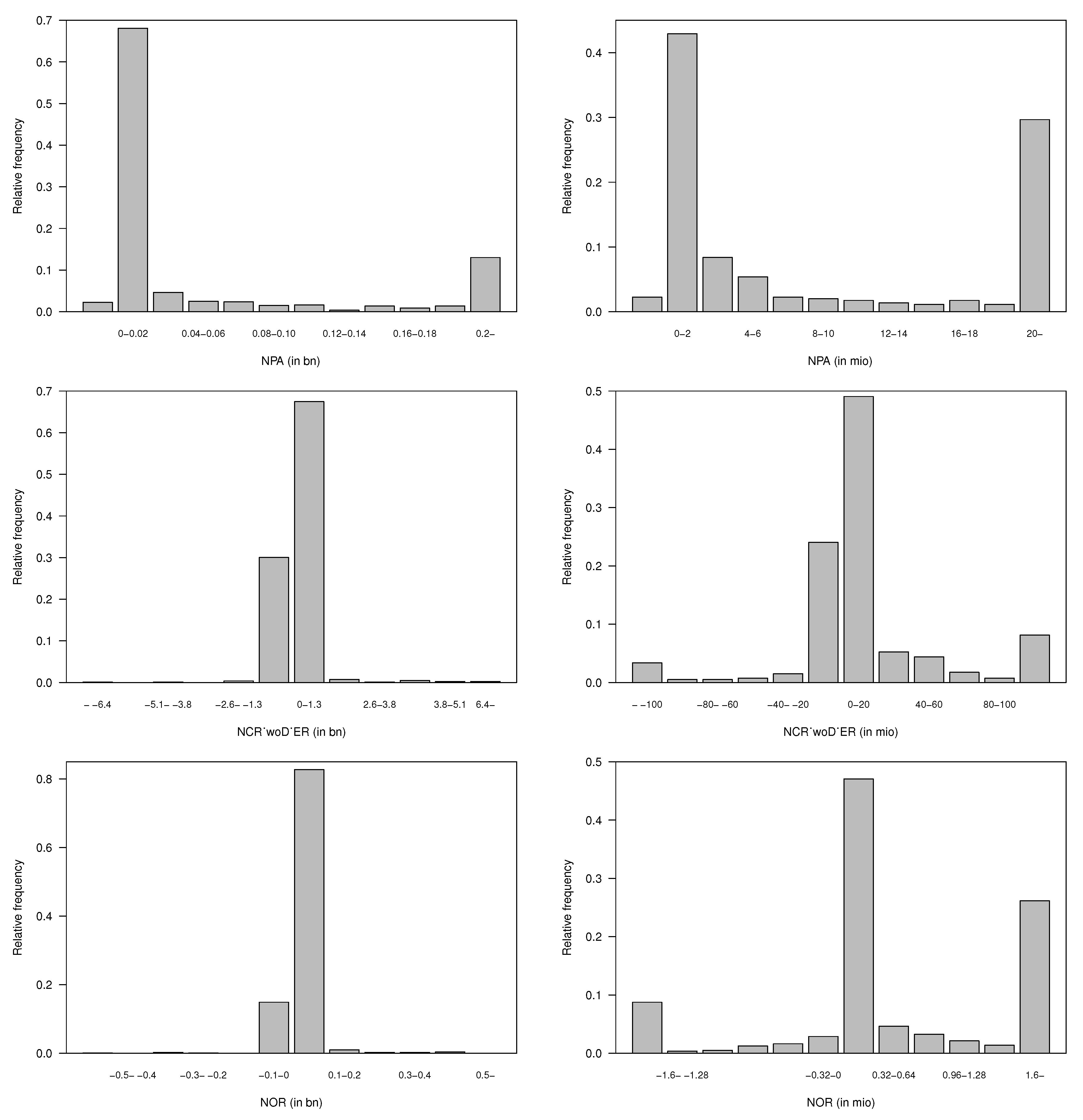
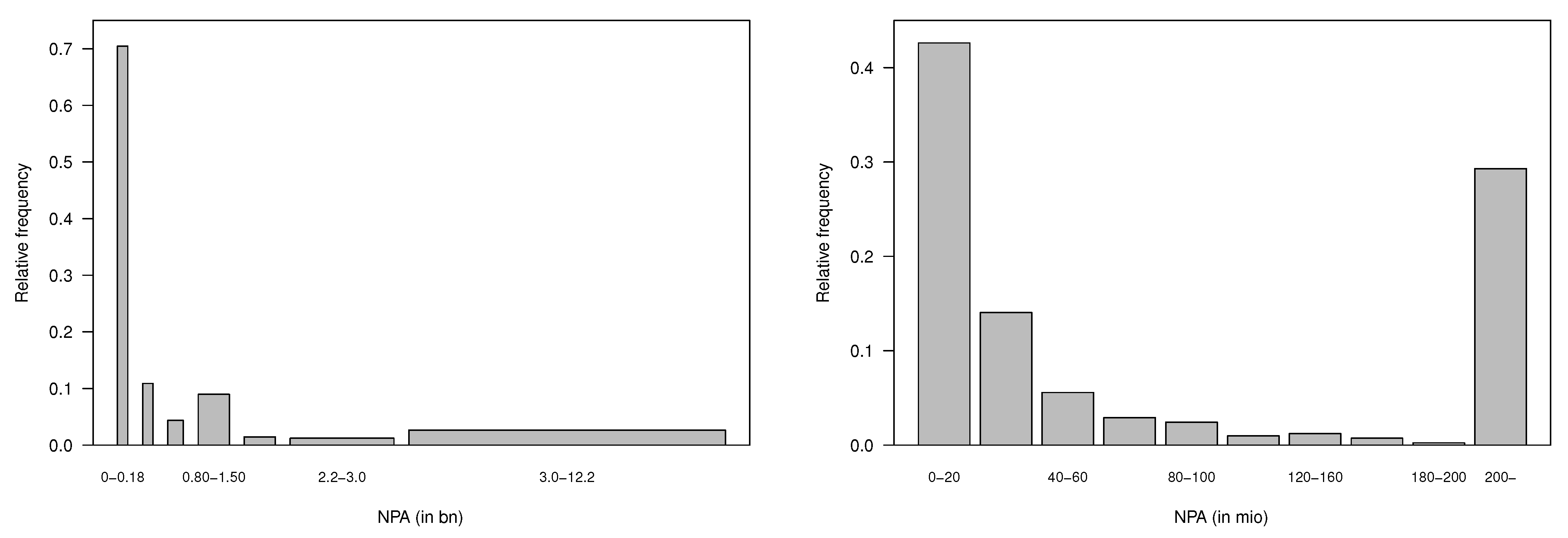
Figure A1 shows the relative frequency of the equalization reserves and of the one of the previous year. In total, 82% report the equalization reserves lower than CHF 24 million, and 82% report the equalization reserves of the previous year lower than CHF 20 million.
Calendar Years and Legal Form
In the year 2007, most observations are noticed; hence, we re-level the variable calendar year to the year 2007. The number of observations in a calendar year increased from 21 in the year 1997 to 62 in the year 2007 and dropped to 34 in the year 2008. In the year 1997, 3% and in the year 2018, 4% of the observations occurred. FOPI published the years 1997 to 2007 and FINMA uses another reporting system for the calendar year 2008 to 2018.
FINMA (
2009) supervised 28 reinsurance undertakings (2007: 25) and 42 captives (2007: 46) in the calendar year 2008; as a consequence, mergers and acquisitions would not explain the drop from the year 2007 to 2008. We think our counting method, companies having a positive equalization reserves, causes the drop: some reinsurance undertakings would have used the occasion of the new reporting system to change the reporting of the equalization reserves.
All analyzed reinsurance undertakings and reinsurance captives are stock companies; therefore, the variable “legal form” would not be suitable for an explanatory one. Instead, we analyze the kind of reinsurance, captive and professional reinsurer. In the year 1997, 38% were captives, increasing to 78% in the year 2011 and dropping to 56% in the year 2018. As more observations for captives are available, we re-level the explanatory variable to “captive”.
Net Earned Premium
The smallest net earned premium amount was CHF −1.3 billion and the highest was CHF 20.3 billion (Swiss Re 2008). Europäische Rückversicherung reported in the year 2005 indeed a higher ceded premium (written: CHF 6.0 billion) than the gross one (written: CHF 5.1 billion), resulting in a negative net earned premium (CHF −1.3 billion). In
Appendix C.1,
Figure A2 displays the relative frequency of the net earned premium and the one of the calendar year. In total, 94% have a net earned premium lower than CHF 2.0 billion and 62% lower than CHF 20 million.
Insurance Costs
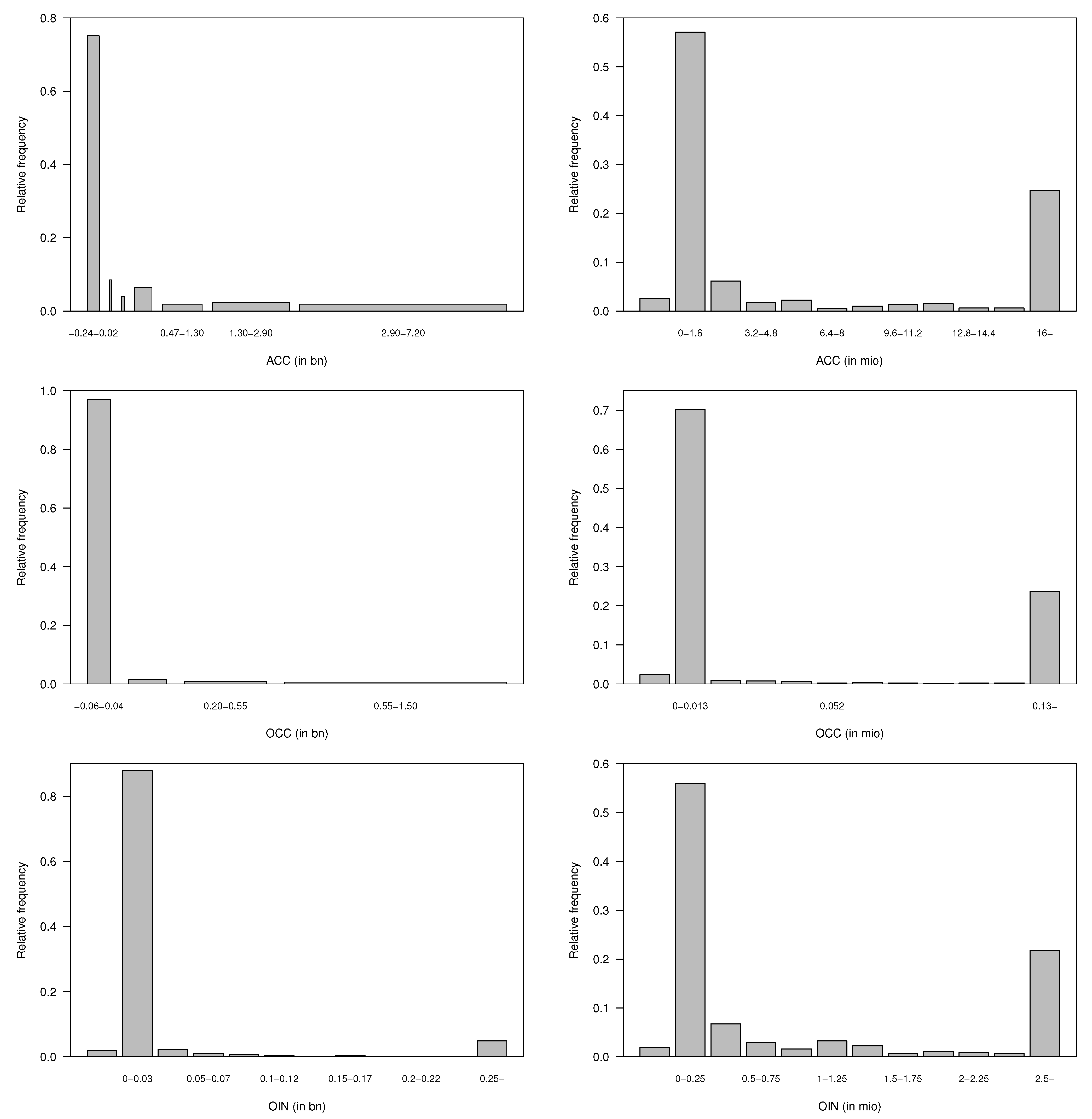
The insurance net claims payments are within the range from CHF −5.6 billion to CHF 20.1 billion (Swiss Re 2009). Europäische Rückversicherung reported in the year 2009 CHF 5.6 billion as payment, having an opposite sign to all other undertakings. In total, 87% have net claims payments lower than CHF 200 million and 70% lower than CHF 20 million. The highest release in claims reserves without change in equalization reserves was CHF 10.7 billion (Swiss Re 2009) and the highest accumulation CHF 8.2 billion (Swiss Re 2016). Furthermore, Swiss Re reported in the year 2017 the highest release in other reserves of CHF 1.3 billion and in the year 2014 the highest accumulation of CHF 429.2 million. In total, 80% report a change in claims reserves without change in equalization reserves in the range from CHF −10.7 billion to CHF 20 million and 62% a change in other reserves in the range from CHF −1.3 billion to CHF 320 million. The relative frequency of the insurance cost of reinsurance undertakings are shown in
Appendix C.1 in
Figure A3.
Operational Costs and Other Technical Income
The operational costs consist of administration cost and commission, being in the range from CHF −0.2 to CHF 7.2 billion (Swiss Re 2006), and other cost, having values from CHF −63.6 million (Swiss Re 2013) to CHF 1.5 billion (Swiss Re 2018). Europäische Rückversicherung reported in the year 2008 CHF −0.2 billion as operational costs, having an opposite sign to all other undertakings. This could occur due to ceded costs from outward reinsurance. Indeed, in the year 2013, Swiss Re reported other costs with a negative sign. Other technical income comprises technical interest income, attributed to the technical part, and other technical insurance income. This item is in the range from CHF −120 million to CHF 2.5 billion (Swiss Re 2007). Europäische Rückversicherung reported in the years 2013 CHF 120 million as other technical income, having an opposite sign to all other undertakings. Due to ceded cost out of outward reinsurance this could happen. In
Appendix C.1,
Figure A4 presents the relative frequency of the operational costs and of the other technical income. In total, 70% of the administration and commission costs are below CHF 8 million, 73% of the other costs are below CHF 13,000 and 69% of the other insurance income is below CHF 1 million.
Technical Result and Company Age
The smallest technical result amounts to a loss of CHF 2.2 billion (Swiss Re 2001) and the highest to CHF 2.1 billion (Swiss Re 2007). A total of 78% report a technical result lower than CHF 6.4 million. In
Appendix C.1,
Figure A5 shows the relative frequency of the technical result and of the company age. The company age is in the range from founded to 135 years. In our analysis, 88% of the companies have a company age below 30.
4.3.2. Model for the Reinsurance Undertakings
Our objective is to find a GAM and a GLM model for the reinsurance undertakings, as presented in
Section 4.2. First, we determine the distribution of the equalization reserves for the reinsurance undertakings. In the second step, we define the GAM model by selecting the explanatory variables. Thereafter, we study the result and apply
evtree to define classifications for explanatory variables. Finally, we apply the GLM model by using the discrete and the transformed variables and present the main results.
Equalization Reserves’ Distribution
As mentioned in
Section 4.2.1, the literature does not propose a class of distribution for the equalization reserves. Therefore, we let our equalization reserves’ observations speak for themselves. We fit some distribution of the exponential family (exponential, Weibull, Gamma and log-normal distribution) on our data and compare the theoretical and the sample quantiles, presented in
Appendix D Figure A11. In
Figure A11, the q-q plots of all fitted distributions are far off the diagonal. The log-normal distribution is the only suitable one; for the other three distributions, insufficient observation points exist to properly fit the tail. In addition, we calculate the AIC values for these distributions, presented in
Table 6. For the reinsurance undertakings, the log-normal distribution best approximates the response variable, equalization reserves.
Selection of the Explanatory Variables to Define GAM
Our goal is to figure out the relationship between the response variable, equalization reserves, with the explanatory variables, as presented in the
Section 4.2.2.
In the previous paragraph, we worked out that equalization reserves could be fitted by a log-normal distribution; thus,
is normal distributed. According to
Wood (
2010) we implement in R a GAM model with the family Gaussian and we use the link function identity, ignoring the correlation of the explanatory variables, as mentioned in
Section 4.2.3.3. We apply the algorithm, outlined in Equation (
12), and obtain the GAM model, as follows:
Equalization reserves of the previous year head the selection of the explanatory variables for reinsurance undertakings. The categorial variable calendar year has the second highest impact on the equalization reserves, according to our approach. Thereafter, the legal form (capitves or professional reinsurers) shapes the equalization reserves. The variable technical result has position four, administration and commission cost position five, and the variable other costs terminate the selection of the explanatory variables, shaping the equalization reserves of the reinsurance undertakings. An additional explanatory variable would not improve the fitting. In
Appendix E,
Table A3 shows the AIC values for the iterations.
In the first column of
Table 7, we list the intercept, the coefficients of the discrete variables, the estimated degree of freedom (edf) of the continuous variables and the significance level of the GAM model. We use the star-notation to mark the statistical significance level of the variables in
Table 7: “.” for a
p-value below 0.1, “*” for a
p-value below 0.05, “**” for a
p-value below 0.01 and “***” for a
p-value below 0.001. The smoothing functions of the continuous variables are statistically significant, the intercept and some coefficients of the discrete variables. As
Fridley (
2010) explains with respect to the GAM model, the predictor variable is separated into sections and fitted by polynomial functions in each section separately. These turning points are measured as edf: the higher the edf, the more complex the smoothing. The continuous variables equalization reserves of the previous year, technical result and the administration and commission costs have an edf-value of 9.0, 7.44 and 8.45, which have the highest complexity to be smoothed. The variable other costs has an edf value of 5.03, which is the lowest complexity to be smoothed. The categorial variable year has 2007 as the base line and the categorial variable legal form has captive as the baseline.
GAM Result and evtree to Define Classifications for Explanatory Variable
Visualization of the fitted smoothing curves reveals the highest insight into the relationship of the explanatory variables on the equalization reserves. As outlined above in Equation (
13), we define the optimal classes of the explanatory variable and in
Table A5 the used parameters of the
evtree are listed. We add this information in
Figure 1: for each explanatory variable its GAM prediction on the equalization reserves is shown (solid line), the 95% confidence interval is marked (dashed lines), the boundaries of the bins are displayed by the vertical lines and the predicted mean effect for each class is indicated by the dashed-pointed horizontal lines.
Equalization Reserves of the Previous Year
Equalization reserves of the previous year are shown in
Figure 1a and we find three classifications. Around 680 companies report the equalization reserves of the previous year lower than CHF 22 million, which has a negative impact on the equalization reserves. The next class is up to CHF 305 million, consisting of around 90 observations, influencing the equalization reserves to increase. The higher the equalization reserves of the previous year, the more equalization reserves are built up. As a take away, we note that the smaller the equalization reserves of the previous year, the more these equalization reserves would be released in the next year. To transform this continuous variable into the discrete one, we define three classes. In the class CHF 0 to 22 million, most observations occur, on which we level this variable.
Calendar Year
In
Figure 1b, the impact of the discrete variable calendar year is displayed and two classes are found. The calendar year is re-leveled to the year 2007. The years could be split in the range 1997 to 2006, having a negative impact on the equalization reserves, and 2008 to 2018, having a positive impact on the equalization reserves. By adding the categorial variable legal form to the GAM model, the year 2017 moved from the class 2008–2018 to 1997–2006 due to a reduction in the equalization reserves of a reinsurer of around CHF 1 billion. In the years 1997 to 2007, FOPI was in charge of the supervision and since 2008, it was FINMA.
Legal Form
Reinsurance undertakings are either captives or professional reinsurance undertakings. Baseline is the category captive. As presented in
Table 7, the coefficient for the professional reinsurer is 1.03: compared to captives, professional reinsurers tend to build more equalization reserves.
Technical Result
The effect of the technical result on the equalization reserves is presented in
Figure 1c, with two classes. The first classification consists of 20 nodes, and the loss of the undertaking is higher than CHF 60 million. The effect on the equalization reserves is negative. The second class comprises 780 observations, and the impact on the equalization reserves is slightly positive. As a take away, we note that for reinsurance undertakings, even positive technical results have only a slightly positive impact on equalization reserves. To transform this continuous variable to the discrete one, we define two classes. As the most observations occur in the class CHF −60 to 2100 million, we level this variable on this class.
Administration and Commission Costs
In
Figure 1d, the effect of the administration and commission costs on the equalization reserves is presented, with seven classes. The first class consists of 600 companies, with administration and commissions costs up to CHF 15 million and a slightly negative impact on the equalization reserves. In the next class, around 70 companies are collected, with costs up to CHF 55 million and a slightly positive impact on the equalization reserves. The class, with costs between CHF 470 million and CHF 1.3 billion, has a negative impact on the equalization reserves, whereby this class consists of 15 observations. The higher the administration and commission costs, the higher the accumulation of the equalization reserves. To transform this continuous variable to the discrete one, we define seven classes. Most observations occur in the class CHF −235 to 15 million on which we level this variable.
Other Costs
Figure 1e presents the effect of other costs on the equalization reserve, with four classes. The first class contains 775 observations with other costs up to CHF 40 million. This class has a sightly negative effect on the equalization reserves. In the second class, 12 companies are captured, having other costs up to CHF 200 million; the impact on equalization reserves is positive. Seven observations are in the third class, having other costs up to CHF 550 and having a higher positive effect on equalization reserve than for the first class. The class number four has five observations, having other costs up to CHF 1.5 billion and a negative effect on equalization reserves. To transform this continuous variable to the discrete one, we define four classes. In the class CHF −64 to 40 million, most observations occur, on which we level this variable.
GLM Model
We apply the GLM model on the initial discrete variables year and legal form and on the initial continuous variables, as transformed and described in the previous paragraph. We mark the transformed variable with “
”, and Equation (
14) turns to the GLM model:
In the second column of
Table 7, we list the intercept, the coefficients of the discrete and of the transformed variables and the significance level of the GLM model. In the GAM model and in the GLM one, the intercept has a statistically significant level “***” and amounts to 14.77 in the GAM and to 14.10 in the GLM one. The significance level of the initial discrete variables either remains the same or changes to the next significance level. All except one coefficient of the initial continuous variables have a significance level of “***” or “**” in the GLM. However, the coefficient of the technical result is not statistically significant in the GLM model. Furthermore, the GAM model has an AIC value of 3218 and the GLM one an AIC value of 3337, making the GAM a better one, see
Table 7.
Result
For reinsurance undertakings, the GAM model performs better than the GLM one. Based on the GAM model, we find the use of equalization reserves: accumulation and release of the equalization reserves are observed. From the GAM and from the GLM model, we note that, compared to captives, professional reinsurers tend to build more equalization reserves. Based on the GAM model, we show that reinsurance undertakings, having small equalization reserves of the previous year, would release the equalization reserves. In addition, from the GAM model, we find that for reinsurance undertakings, even positive technical results have only a small positive impact on equalization reserves.
4.4. Model of the Equalization Reserves for Non-Life Undertakings
To explore the equalization reserves for non-life undertakings, we base the analysis on FOPI data. In
Section 4.4.1, we look at the data, and thereafter, in
Section 4.4.2, we present the model result using the approach described in
Section 4.2.
4.4.1. Data for Non-Life Undertakings
FOPI published the equalization reserves for non-life undertakings for the calendar years 1997 to 2007. For our analysis we filter the data points, having positive equalization reserves, and 413 data points are available for our study.
Table 8 captures the summary of the equalization reserves and of the explanatory variables, covering the years 1997 to 2007. The currency is CHF. Minimum (Min.), first quantile (1st Qu.), median, mean, third quantile (3rd Qu.) and maximum (Max.) are presented.
Equalization Reserves
The smallest equalization reserves amount to CHF 1000 and the highest to CHF 375.4 million (Mobiliar 2004). In
Appendix C.2,
Figure A6 shows the relative frequency of the equalization reserves and of the one of the previous year. In total, 70% report the equalization reserves lower than CHF 40 million, and 71% report the equalization reserves of the previous year lower than CHF 30 million. For the year 1997, information regarding the equalization reserves of the previous year could not be calculated and the analysis will lack this item for the year 1997.
Calendar Years and Legal Form
In the year 1998, most observations are made; hence, we re-level the variable calendar year to the year 1998. The number of non-life entities were reduced, on the one hand, due to mergers and acquisition and, on the other hand, due to our selection criteria, analyzing records with positive equalization reserves. In the year 1997, 10% and, in the year 2007, 8% of the observations occurred. The share of mutual companies increased from 15% in the year 1997 to 25% in year 2007.
Net Earned Premium
The smallest net earned premium amounted to CHF −12,140 and the highest to CHF 22.8 billion (Zurich 2008). Unifun reported in the years 2004 and 2005 a higher ceded premium than the gross one, resulting in a negative net earned premium. In
Appendix C.2,
Figure A7 displays the relative frequency of the net earned premium and the one of the calendar year. In total, 70% have a net earned premium lower than CHF 353.9 million and 47% lower than CHF 40 million.
Insurance Costs
The insurance net claims payments are within the range from CHF 0 (Polygon) to CHF 12.2 billion (Zurich 2007). In the year 2003, Baloise reported the highest release in claims reserves without change in equalization reserves of CHF 314.5 million, and in the year 2003, Zurich reported the highest accumulation of CHF 3.98 billion. Furthermore, the highest release in other reserves was CHF 40.1 million (Mobiliar 2005) and the highest accumulation CHF 379.1 million (Zurich 2006). The relative frequency of the insurance cost of non-life undertakings is shown
Appendix C.2 in
Figure A8. In total, 70% have net claims payments lower than CHF 823.3 million and 43% lower than CHF 20 million. Furthermore, 60% report a change in claims reserves without change in equalization reserves in the range from CHF −15.1 million to CHF 11.7 million.
Operational Costs and Other Technical Income
The operational costs consist of administration cost and commission, being in the range from CHF −0.2 million (Appenzeller 1997) to CHF 6.3 billion (Zurich 2007), and other costs, having values from CHF −27,034 (Orion 2006) to CHF 327.6 million (Zurich 2004). Appenzeller received more compensation for the cost from the ceded reinsurance contract than indeed paid, resulting in a negative administration and commission cost. Indeed, Orion reported other costs with a negative sign. Other technical income comprises technical interest income, attributed to non-life insurance, and other technical insurance income; this item is in the range from CHF −18.4 million (Vaudoise 2002) to CHF 2.5 billion (Zurich 1998). Vaudoise reported in the year 2002 a negative technical interest income of CHF 20.2 million compensated by a positive other technical insurance income of CHF 1.8 million. In
Appendix C.2,
Figure A9 presents the relative frequency of the operational costs and of the other technical income. In total, 72% of the administration cost and commission are below CHF 99.8 million, 73% of the other costs are below CHF 0.6 million and 73% of the other insurance income is below CHF 21.6 million.
Technical Result and Company Age
Zurich reported in the year 2002 the highest technical loss of CHF 1.2 billion and in the year 2006 Zurich had the highest technical result of CHF 2.4 billion. In
Appendix C.2,
Figure A10 shows the relative frequency of the technical result and of the company age. In total, 70% report a technical result lower than CHF 5 million. The company age is in the range from founded to 181 years. In our analysis, 67% of the companies have a company age below 100.
4.4.2. Model of the Non-Life Undertakings
Our objective is to find a GAM and a GLM for the non-life undertakings, as presented in
Section 4.2. First, we determine the distribution of the equalization reserves for the non-life undertakings. In a second step, we define the GAM by selecting the explanatory variables. Thereafter, we study the result and apply
evtree to define classifications for explanatory variables. Finally, we apply the GLM by using the discrete and the transformed variables and present the main results.
Equalization Reserves’ Distribution
Like the reinsurance procedure, we let our equalization reserves observations speak for themselves. We fit the exponential, Weibull, Gamma and log-normal distribution, being of the exponential distribution family, on our data and compare the theoretical and the sample quantiles, presented in
Appendix D Figure A12. Furthermore, we calculate the AIC values for these distributions, presented in
Table 9. For the non-life undertakings, the Gamma distribution best approximates the response variable, equalization reserves.
Selection of Explanatory Variables to Define GAM
Our goal is to figure out the relationship between the response variable, equalization reserves, with the explanatory variables, as presented in
Section 4.2.2.
In the previous paragraph, we worked out that equalization reserves could be fitted by a Gamma distribution. According to
Wood (
2010), we implement in R a GAM model with the family Gamma and we use the link function
, ignoring the correlation of the explanatory variables, as mentioned in
Section 4.2.3.3. We apply the algorithm, outlined in Equation (
12), and obtain the GAM model, as follows:
Net claims payments head the selection of the explanatory variables. The equalization reserves of the previous year have the second-highest impact on the equalization reserves. Thereafter, the net change in claim reserve without change in equalization reserves shapes the equalization reserves. The categorial variable calendar year has position four, and the net earned premium terminates the selection of the explanatory variables, impacting the equalization reserves of the non-life undertakings. An additional explanatory variable would not improve the fitting. In
Appendix E,
Table A4 presents the AIC values for the iterations.
In the first column of
Table 10, we list the intercept, the coefficient of the categorial variables, the edf of the continuous variables and the significance levels of the GAM model. We use the star-notation to mark the statistical significance of the variables in
Table 10. The smoothing function of the net claims payments has significance code “**”, whereby the smoothing functions of the continuous variables equalization reserves of the previous year, net change in claim reserves without change in equalization reserves and net earned premium have each the significance code “***”. Thus, all smoothing functions of the continuous variables are statistically significant. In addition, the intercept and the coefficient of the year 1997 are statistically significant. The continuous variables equalization reserves of the previous year and the net change in claim reserves without equalization reserves have an edf value of 8.79 and 7.88, having the highest complexity to be smoothed. Net claims payments and net earned premium have an edf value of 4.94 and 3.41, having the lowest complexity to be smoothed. The categorial variable year has 1998 as the baseline.
GAM Result and evtree to Define Classifications for Explanatory Variable
Visualization of the fitted smoothing curves reveals the highest insight into the relationship of the explanatory variables on the equalization reserves. As outlined above in Equation (
13), we defined the optimal classes of the explanatory variable and in
Appendix F in
Table A6 the used parameters of the
evtrees are listed. We added this information in
Figure 2: for each explanatory variable of the selection, its GAM prediction on the equalization reserves is shown (solid line), the 95% confidence interval is marked (dashed lines), the boundaries of the bins are displayed by the vertical lines and the predicted mean effect for each class is indicated by the dashed-pointed horizontal lines.
Net Claims Payments
Net claims payments are shown in
Figure 2a, and we find seven classes. Around 300 claims payments, being lower than CHF 180 million, have a negative impact on the equalization reserves. The next class is up to CHF 470 million claims payments, consisting of 45 observations without any impact on the equalization reserves. The higher the claims payments of the company the more equalization reserves are built up. As a take away, we note that companies with small claims payments tend to release equalization reserves, and the ones with high claims payments tend to establish more equalization reserves. To transform this continuous variable into the discrete one, we define seven classes. Most observations occur in the class CHF 0–180 million, on which we level this variable.
Equalization Reserves of the Previous Year
In
Figure 2b, the impact of the equalization reserves of the previous year is displayed and eight classes are marked. The first class has around 130 companies, having equalization reserves of the previous year lower than CHF 2.0 million. Its impact on the equalization reserves is negative; small companies more often release the equalization reserves of the previous year to finance the claims. Each of the remaining seven classes have around 40 nodes. To transform this continuous variable to the discrete one, we define eight classes. In the class CHF 0–2.0 million, most observations occur, on which we level this variable.
Net Change in Claim Reserves without Change in Equalization Reserves
Net change in claim reserves without change in equalization reserves is presented in
Figure 2c and has eight classes. The first classification consists of 20 nodes and the release in claim reserves is higher than CHF 20 million; the effect on the equalization reserves is negative. The next class has around 250 observations covering the release of claim reserves up to CHF 20 million and the accumulation of claim reserves up to CHF 11 million. The average effect on equalization reserves is negative. Within the third class, the claim reserve would accumulate up to CHF 37 million, whereby the impact on the equalization reserves would still be negative half as much as in the second class. The higher the accumulation of claim reserves of the company, the more equalization reserves are built up. Releasing of claim reserves impacts a release in equalization reserves; an accumulation of claim reserves higher than CHF 35 million would impact an accumulation of equalization reserves. In consequence, a small accumulation of claim reserves up to CHF 35 million would shift the reserves from equalization to claim. To transform this continuous variable to the discrete one, we define eight classes. In the class CHF −20–11 million, most observations occur, on which we level this variable.
Calendar Year
In
Figure 2d, the effect of the calendar year on the equalization reserves is presented; no
evtree could be found. The baseline is the year 1998. As for the year 1997, information regarding the equalization reserves of the previous year is missing, and the effect of the year 1997 on the equalization reserves could not be observed. All other years have a small effect on the equalization reserves.
Net Earned Premium
Net earned premium is presented in
Figure 2e, having five classes. The first class contains around 290 observations up to CHF 300 million net earned premium. This class has a positive effect, being close to 2, on the equalization reserves. In the second class, around 60 companies are captured up to a net earned premium to CHF 1000 million, and the effect is slightly negative. The higher the net earned premium of the company, the fewer equalization reserves are built up. To transform this continuous variable to the discrete one, we define eight classes. In the class CHF 0–300 million, most observations occur, on which we level this variable.
GLM Model
We apply the GLM model on the initial discrete variables year and legal form and on the initial continuous variables as transformed and described in the previous paragraph. We mark the transformed variable with “
” and Equation (
16) turns to the GLM model:
In the second column of
Table 10, we list the intercept, the coefficients of the discrete and of the transformed variables and the significance level of the GLM model. In the GAM and GLM models, the intercept of the initial discrete variable year has a statistically significant level “***” and amounts to 16.35 for the GAM model and 13.86 for the GLM one. For the discrete variable year in the GLM model, only one coefficient has a statistically significant level “*” and the other years are not significant. All coefficients of the initial continuous variables
and
have a significance level of “***” or “*” in the GLM model. Two coefficients of net claims payments have a statistical significant level “**” and “*”; the others are not significant in the GLM model.
In the GLM model for the initial continuous variable net earned premium, three coefficients could not be defined, as net earned premium and net claims payments have an exact linear relationship between them. In
Section 4.2.2, we explain how to select the best GAM model by looking at the AIC values. In
Appendix E Table A4, we present the AIC values: in the first iteration, the AIC value of the net earned premium is 14,948, while AIC of the net claims payments is 14,944. The net claims payments are the best explanatory variable in the first iteration and the net earned premium is selected in the last iteration. We cannot explain why the last iteration, selecting the net earned premium as the explanatory variable, should improve the GAM model. This is a limitation of our paper.
The AIC values of the GAM and GLM models are reported in
Table 7: the GAM model has an AIC value of 14,485 and the GLM one has an AIC value of 14,454, making the GLM a better one.
Result
For non-life undertakings, the GLM performs better than the GAM model. Our approach to select the best GAM model by looking at AIC values has not detected the strong relationship between net earned premium and net claims payments. Based on the GAM model, we find the use of equalization reserves: accumulation and release of the equalization reserves are observed. From the GAM model, we notice an opposite effect between small-sized and large-sized non-life companies: for small-sized companies, the release effect is observed regarding the insurance expenses, whereby the premium income variable indicates an accumulation one. For large-sized companies, the release effect is observed regarding the premium income variable, whereby the insurance expenses indicate an accumulation effect. Based on the GAM model, we note that non-life undertakings, having small equalization reserves of the previous year, would release the equalization reserves.
5. Discussion
One result of this paper is that the Swiss equalization reserves could be restated out of the publicly available figures for the years 1997 to 2018 for reinsurance undertakings and for the years 1997 to 2007 for the non-life undertakings, although the equalization reserves are not explicitly published. We detect that profit and loss items are identified as explanatory variables for the equalization reserves and that the equalization reserves could not be misused for tax optimization by defining the upper limit and their accumulation and their release. Undertakings need the equalization reserves.
In the literature, the Swiss equalization reserves are not studied, and Swiss undertakings do not publish how their equalization reserves are handled. This paper fills the gap and starts the discussion about the equalization reserves.
Disclosing the equalization reserves reveals the financial cushion of the undertaking and could awaken the covetousness of some greedy short-term investors.
Equalization reserves should smooth the volatility of the case reserves, which should be studied in detail, being a further research topic. Another further research topic could be a study about the determination of the optimal upper limit of the equalization reserves. The basis of this paper is the restated equalization reserves. Thus, the study could be enriched by using the equalization reserves reported by the undertakings. In addition, a future research direction could be the impact of the equalization reserves on the (tied) assets.
6. Conclusions
In this paper, we use publicly available data from FOPI and FINMA to restate the equalization reserves for the years 1997 to 2018 for reinsurance and for non-life undertakings in Switzerland and we analyze the relationship between these equalization reserves and the profit and loss items, using a GAM and a GLM model. The analysis is limited to 799 observations for reinsurance undertakings and to 413 observations for non-life undertakings.
For reinsurance undertakings, the equalization reserves depend on the equalization reserves of the previous year, on the calendar year, on the legal form, on the technical result, on the administration and commission costs and on other costs. The GAM model performs better than the GLM one for reinsurance undertakings. For non-life undertakings, the equalization reserves depend on the net claims payments, on the equalization reserves of the previous year, on the net change in claims reserves without change in equalization reserves, on the calendar year and on the net earned premium. The GLM model performs better than the GAM one, for non-life undertakings.
We figure out the use of the equalization reserves for reinsurance and for non-life undertakings: accumulation and release of the equalization reserves are observed. Based on the GAM model, we note that reinsurance and non-life undertakings, having small equalization reserves of the previous year, would release the equalization reserves. From the GAM and from the GLM model, we note that, compared to captives, professional reinsurers tend to build more equalization reserves.
We illustrated that by fixing the accumulation and the release of the equalization reserves within the business plan, no tax advantage could be gained out of the equalization reserves. The equalization reserves belong to the policyholder and to the portfolio.
The discussion about the disclosing of the equalization reserves should be restarted.
After finding a positive consensus, the analysis could be repeated based on more observations and real figures.
Reinsurance and non-life undertakings should reflect whether the definition of the equalization reserves, fixed in the business plan, should be linked to the outcome of the capital modeling for insurance/reserving risk or linked to other profit and loss items or on a mixture of both.
Another future research question could be derived: do the equalization reserves impact the variance of the technical reserves within the statutory accounts for an undertaking? Furthermore, a future research topic could be the missing explanation as to why the last iteration improves the GAM model when defining the best GAM model, whereby the selected last explanatory variable is highly correlated to an already identified one.
The work is limited to publicly available data, whereby the equalization reserves were restated. To improve the GAM and the GLM model, the database should take the reported equalization reserves as a basis. First, this would enlarge the number of observations the analysis is based on. Second, the restated equalization reserve could be replaced by the observation, avoiding unnecessary inaccuracies.
Author Contributions
Conceptualization, A.B.; methodology, A.B.; software, A.B. and Y.S.; validation, A.B.; formal analysis, A.B.; investigation, A.B.; data curation, A.B.; writing—original draft preparation, A.B.; writing—review and editing, A.B.; visualization, A.B.; supervision, A.B.; project administration, A.B. All authors have read and agreed to the published version of the manuscript.
Funding
This research received no external funding.
Institutional Review Board Statement
Not applicable.
Informed Consent Statement
Not applicable.
Data Availability Statement
Acknowledgments
The authors are very thankful to Joël Wagner for his helpful comments and suggestions and for organizing the funding of the publication.
Conflicts of Interest
The authors declare no conflict of interest.
Appendix A. Main Changes within FOPI’s and FINMA’s Reporting
The appendix starts in
Appendix A with a short overview of the main changes within FOPI’s and FINMA’s reporting. In
Appendix B the source of the available explanatory variables within the R model is presented: once for FOPI in
Table A1 and once for FINMA in
Appendix B.2. Thereafter, in
Appendix C the relative frequency of all available explanatory variables is presented: once for reinsurance undertakings in
Appendix C.1 and once for non-life undertakings in
Appendix C.2. In
Appendix D the fit of the response variable’s distribution function, equalization reserves, is depicted for reinsurance and for non-life undertakings. Then, in
Appendix E the AIC values for reinsurance and for non-life undertakings are shown. Finally, in
Appendix F the parameters of the
evtree for reinsurance and for non-life undertakings are listed.
FOPI and FINMA have disclosed the figures in a slightly different setup. The main changes are:
For life undertakings, FINMA changed the presentation of the number of individual and collective contracts and the sum insured, written directly in Switzerland;
For non-life undertakings, FINMA changed the presentation of the number of contracts and number of risks, written directly in Switzerland;
For life and for non-life undertakings, FINMA changed the presentation of the equalization reserves, written directly in Switzerland;
For life undertakings, FINMA publishes the written periodic premium of the direct business in Switzerland;
FOPI published the number of workers within the insurance industry;
FOPI published the profit and loss and the balance sheet information of each single (re-)insurance, undertaking each in one file. Furthermore, FOPI published these gross and net items; FINMA publishes only the net ones;
For non-life undertakings, FOPI published tied assets information, whereas FINMA publishes tied assets for life and non-life undertakings within one file. Furthermore, the composition of “Sollbetrag” changed over time.
Appendix B. Source of the Available Explanatory Variables
Appendix B.1. FOPI’s Available Explanatory Variables
Table A1.
FOPI published the files “Jahresrechnungen” in each calendar year for each undertaking. This is the source of the available explanatory variables for reinsurance and non-life undertakings.
Table A1.
FOPI published the files “Jahresrechnungen” in each calendar year for each undertaking. This is the source of the available explanatory variables for reinsurance and non-life undertakings.
| Variable | FOPI’s Title and Calculation | Cell |
|---|
| Aufwendungen für den Versicherungsbetrieb für eigene Rechnung | C32 |
| Calendar Year - Foundation Year (as stated in Zefix) | |
| Included in the name of the undertaking (as stated in Zefix) | |
| Veränderung der Schadenrückstellungen für eigene Rechnung | C19 |
| | | |
| Verdiente Prämien für eigene Rechnung | C9 |
| Nicht anderweitig auszuweisende Veränderung vt. Nettorückstellungen | C21 |
| Zahlungen für Versicherungsfälle für eigene Rechnung | C16 |
| Nicht realisierte Verluste aus Kapitalanlagen für anteilgebundene Lebensversicherungen | C33 |
| | Sonstige vt. Aufwendungen für eigene Rechnung | C34 |
| | | |
| Der technischen Rechnung zugeordneter Zinsertrag für eigene Rechnung | C10 |
| | Nicht realisierte Gewinne aus Kapitalanlagen für anteilgebundene Lebensversicherungen | C11 |
| | Sonstige vt. Erträge für eigene Rechnung | C12 |
| | | |
| Ergebnis der vt. Rechnung | C35 |
| Calendar Year | |
Appendix B.2. FINMA’s Available Explanatory Variables
Table A2.
FINMA published the data within a “cube” for the years 2008 to 2018. Section “Bilanz and Erfoglsrechnung” is the source of the available explanatory variables for reinsurance and non-life undertakings.
Table A2.
FINMA published the data within a “cube” for the years 2008 to 2018. Section “Bilanz and Erfoglsrechnung” is the source of the available explanatory variables for reinsurance and non-life undertakings.
| Variable | FINMA’s Title and Calculation | Section |
|---|
| Aufwendungen für den Versicherungsbetrieb für eigene Rechnung | Erfolgsrechnung - Aufwand |
| Calendar Year - Foundation Year (as stated in Zefix) | |
| Included in the name of the undertaking (as stated in Zefix) | |
| Veränderung der Rückstellungen für Versicherungsfälle/ | Erfolgsrechnung - Aufwand |
| | Schadenrückstellungen (Leben und Schaden) | vt. Aufwand |
| | | |
| Versicherungstechnische Erträge | Erfolgsrechnung - Ertrag |
| Veränderung der übrigen vt. | Erfolgsrechnung - Aufwand |
| Verbindlichkeiten für eigene Rechnung (Leben) | vt. Aufwand |
| | |
| Veränderung der übrigen vt. | Erfolgsrechnung - Aufwand |
| Verbindlichkeiten für eigene Rechnung (Schaden) | vt. Aufwand |
| | |
| | |
| Zahlungen für Versicherungsfälle für eigene Rechnung | Erfolgsrechnung - Aufwand |
| | (Leben und Schaden) | vt. Aufwand |
| Sonstige Aufwendungen aus der Versicherungstätigkeit | Erfolgsrechnung - Aufwand |
| Sonstige Erträge aus der Versicherungstätigkeit | Erfolgsrechnung - Ertrag |
| vt. Aufwendungen | Erfolgsrechnung - Aufwand |
| | | |
| | | |
| Calendar Year | |
Appendix C. Relative Frequency
Appendix C.1. Relative Frequency—Reinsurance Undertakings
Figure A1.
Relative frequency of the equalization reserves () and of the one of the prior year () for reinsurance undertakings. The figure presents twice the relative frequency of : once sliced by the optimal bin out of our model and once sliced by equal bands, whereby the last band includes all remaining higher observations.
Figure A2.
Relative frequency of the net earned premium () and of the calendar year () of reinsurance undertakings. The figure presents twice the relative frequency of the : once sliced by billion and once sliced by million, whereby the last band includes all remaining higher observations.
Figure A2.
Relative frequency of the net earned premium () and of the calendar year () of reinsurance undertakings. The figure presents twice the relative frequency of the : once sliced by billion and once sliced by million, whereby the last band includes all remaining higher observations.
Figure A3.
Relative frequency of the insurance cost for reinsurance undertakings: net claims payments (), net change in claim reserves without change in () and net change in other technical reserves (). The figure presents twice the relative frequency of the , and : once sliced by billion and once sliced by million, whereby the last band includes all remaining higher observations.
Figure A4.
Relative frequency of the operation cost, administration cost and commission () and other costs (), and of the other income () for reinsurance undertakings. The figure presents twice the relative frequency of , and : and are once sliced by the optimal bin out of our model and once sliced by equal bands. is once sliced by billion and once sliced by million.
Figure A5.
Relative frequency of the technical result () and of the company age () for reinsurance undertakings.
Figure A5.
Relative frequency of the technical result () and of the company age () for reinsurance undertakings.
Appendix C.2. Relative Frequency—Non-Life Undertakings
Figure A6.
Relative frequency of the equalization reserves () and of the one of the prior year () for non-life undertakings. The figure presents twice the relative frequency of : once sliced by the optimal bin out of our model and once sliced by equal bands, whereby the last band includes all remaining higher observations.
Figure A7.
Relative frequency of the net earned premium () and of the calendar year () for non-life undertakings. The figure presents twice the relative frequency of the : once sliced by the optimal bin out of our model and once sliced by equal bands, whereby the last band includes all remaining higher observations.
Figure A8.
Relative frequency of the insurance cost for non-life undertakings: net claims payments (), net change in claim reserves without change in () and net change in other technical reserves (). The figure presents twice the relative frequency of the and : once sliced by the optimal bin out of our model and once sliced by equal bands, whereby the last band includes all remaining higher observations. is sliced in two different intervals.
Figure A9.
Relative frequency of the operation cost, administration cost and commission () and other costs (), and of the other income () for non-life undertakings. The figure presents twice the relative frequency of , and : and are once sliced by billion and once sliced by million. is sliced in two different intervals.
Figure A10.
Relative frequency of the technical result () and of the company age () of non-life undertakings. The figure presents twice the relative frequency of : once sliced by billion and once sliced by million.
Figure A10.
Relative frequency of the technical result () and of the company age () of non-life undertakings. The figure presents twice the relative frequency of : once sliced by billion and once sliced by million.
Appendix D. Fit of the Distribution Function of the Equalization Reserves
Figure A11.
Fit of distribution of the equalization reserves for reinsurance undertakings.
Figure A11.
Fit of distribution of the equalization reserves for reinsurance undertakings.
Figure A12.
Fit of distribution of the equalization reserves for non-life undertakings.
Figure A12.
Fit of distribution of the equalization reserves for non-life undertakings.
Appendix E. Model Output—AIC Values
Table A3.
AIC values of the explanatory variables for the reinsurance undertakings.
Table A3.
AIC values of the explanatory variables for the reinsurance undertakings.
| AIC | Iteration 1 | Iteration 2 | Iteration 3 | Iteration 4 | Iteration 5 | Iteration 6 |
|---|
| 3761 | 3466 | 3303 | 3257 | 3232 | 0 |
| 3894 | 3466 | 3354 | 3262 | 3252 | 3259 |
| 3528 | 0 | 0 | 0 | 0 | 0 |
| 3888 | 3468 | 3289 | 0 | 0 | 0 |
| 3854 | 3519 | 3378 | 3274 | 3247 | 3224 |
| 3742 | 3466 | 3312 | 3257 | 3241 | 3233 |
| 3885 | 3521 | 3402 | 3286 | 3256 | 3234 |
| 3744 | 3478 | 3314 | 3261 | 3249 | 3234 |
| 3885 | 3518 | 3401 | 3283 | 3248 | 3218 |
| 3824 | 3507 | 3343 | 3264 | 3241 | 3221 |
| 3816 | 3489 | 3357 | 3256 | 0 | 0 |
| 3820 | 3406 | 0 | 0 | 0 | 0 |
Table A4.
AIC values of the explanatory variables for the non-life undertakings.
Table A4.
AIC values of the explanatory variables for the non-life undertakings.
| AIC | Iteration 1 | Iteration 2 | Iteration 3 | Iteration 4 | Iteration 5 |
|---|
| 14,952 | 14,895 | 14,929 | 14,585 | 14,493 |
| 15,076 | 14,995 | 14,677 | 14,643 | 14,608 |
| 14,999 | 14,793 | 0 | 0 | 0 |
| 14,971 | 14,942 | 14,591 | 0 | 0 |
| 14,948 | 14,946 | 14,930 | 14,572 | 14,485 |
| 15,020 | 14,948 | 14,932 | 14,583 | 14,501 |
| 14,944 | 0 | 0 | 0 | 0 |
| 15,006 | 14,949 | 14,992 | 14,588 | 14,500 |
| 15,003 | 14,908 | 14,866 | 14,593 | 14,501 |
| 15,000 | 14,946 | 14,926 | 14,593 | 14,502 |
| 15,070 | 14,957 | 14,674 | 14,500 | 0 |
| 15,052 | 14,828 | 14,747 | 14,592 | 14,502 |
Appendix F. Parameters of evtree
Table A5.
Parameters of the evtree for reinsurance undertakings.
Table A5.
Parameters of the evtree for reinsurance undertakings.
| Reinsurance |
|---|
| Explanatory | A | | B | | # Classes |
|---|
| Variables |
|---|
|
| 2 | | 30 | 3 |
| 950 | | 10 | 2 |
| 950 | | 20 | 2 |
| 1 | | 15 | 7 |
| 15 | | 5 | 4 |
Table A6.
Parameters of the evtree for non-life undertakings.
Table A6.
Parameters of the evtree for non-life undertakings.
| Non-Life |
|---|
| Explanatory | A | | B | | # Classes |
|---|
| Variables |
|---|
|
| 1 | | 5 | 7 |
| 4.5 | | 15 | 8 |
| 2.5 | | 10 | 8 |
| 7 | | 10 | 5 |
Notes
| 1 | In German: Versicherungsaufsichtsgesetz—VAG, see ISA ( 2006). |
| 2 | In German: Aufsichtsverordnung—AVO, see ISO ( 2006). |
| 3 | In FINMA ( 2011) the German expression “Schwankungsrückstellungen” is used. |
| 4 | For non-life undertakings the German expression “Sicherheits- und Schwankungsrückstellungen” is used to reflect the nature of the reserves “safety” and “fluctuation”. In this paper we simplify this expression by using the name “equalization reserves”; however, another reasonable name would be “fluctuation reserves”. |
| 5 | |
| 6 | |
| 7 | With respect to Art. 958 of OR, the financial statements comprise balance sheet, profit and loss accounts and the notes of these accounts; the financial statements “must be signed by the chair-person of the supreme management or administrative body and the person responsible for financial reporting within the undertaking”. |
| 8 | The statutory accounting is the basis for the calculation, see FINMA ( 2019c), whereby the Swiss Code of Obligations (OR) regulates the statutory accounting, see Swiss Confederation ( 1912). |
| 9 | For the years 1997 to 2018, the structure of the name of the statistical files is, as follows: two letters, two figures, followed by one letter. The first two letters mark the type of insurance such as reinsurance or non-life undertakings. The two figures refer to the line of business, in general. The last letter indicates the reporting item, in general. |
| 10 | In German: “Pauschalrückstellung”. |
| 11 | In order to keep the terminology simple, we use the word “reinsurance” designated for both captives and for professional reinsurers. In the subsection for reinsurance, we are more precise. |
| 12 | Burnham and Anderson ( 2004) study AIC and explain the relationship between reasonable data and a good model by separating “information” and “noise”. “Here, information relates to the structure of relationships, estimates of model parameters, and components of variance. Noise, then, refers to the residuals: variation left unexplained.” Burnham and Anderson ( 2004). |
| 13 | To cite Fridley ( 2010): “GAMs take each predictor variable in the model and separate it into sections (delimited by ‘knots’), and then fit polynomial functions to each section separately, with the constraint that there are no kinks at the knots (second derivatives of the separate functions are equal at the knots).”. |
| 14 | Simplicity within the notation is made; for we define . Furthermore, we neglect that categorial variables should not have any smoothing functions. |
| 15 | Grubinger et al. ( 2014) explain that the parameter alpha of an evtree “regulates the complexity part of the cost function. Increasing values of alpha encourage decreasing tree sizes.”. |
| 16 | Notation is simplified: e.g., CHF 3.53 billion (Swiss Re 2001) is the shortcut for “the reinsurance undertaking Swiss Re reports in the calendar year 2001 CHF 3.53 billion”. |
References
- Akhurst, Ron, Kathryn Morgan, George Orros, Jonathan Piper, Peter Hinton, Andrew Macnair, Teivo Pentikainen, Joachim Hertig, Charles Levi, Arne Sandström, and et al. 1992. Equalisation Reserves on a European Basis [Conference]. General Insurance Convention. Available online: https://www.actuaries.org.uk/system/files/documents/pdf/0393-0461.pdf (accessed on 2 October 2019).
- Burnham, Kenneth Paul, and David Anderson. 2004. Multimodel Inference: Understanding AIC and BIC in Model Selection. Sociological Methods & Research 33: 261–304. [Google Scholar]
- Dacorogna, Michel, Hansjörg Albrecher, Michael Moller, and Suzane Sahiti. 2013. Equalization reserves for natural catastrophes and shareholder value: A simulation study. European Actuarial Journal 3: 1–21. [Google Scholar] [CrossRef] [Green Version]
- De Vylder, Florian, and Marc Goovaerts. 1999. Solvency margins and equalization reserves. Insurance: Mathematics and Economics 24: 103–15. [Google Scholar] [CrossRef]
- Dunne, Carla, Donal Lehane, Eimear McCarthy, Angela McNally, Maaz Mushir, Ciara Regan, and David Walsh. 2017. IFRS 17 Insurance Contracts: Impacts for Reserving. 2 August 2017. Deloitte & Touche. Available online: https://de.scribd.com/document/379850262/Ie-2017-IFRS-17-Impacts-for-Reserving-Deloitte-Ireland (accessed on 7 October 2019).
- England, Peter, Richard Verrall, and Mario Valentin Wüthrich. 2019. On the lifetime and one-year views of reserve risk, with application to IFRS 17 and Solvency II risk margins. Insurance: Mathematics and Economics 85: 74–88. [Google Scholar] [CrossRef]
- European Insurance and Occupational Pensions Authority (EIOPA). 2015. Guidelines on the Valuation of Technical Provisions. Available online: https://www.eiopa.europa.eu/sites/default/files/publications/eiopa_guidelines/tp_final_document_en.pdf (accessed on 4 September 2018).
- Farny, Dieter. 2011. Versicherungsbetriebslehre. Karlsruhe: Verlag Versicherungswirtschaft. [Google Scholar]
- Federal Office of Private Insurance. 2007. Facts and Figures [Webside]. Available online: https://www.finma.ch/FinmaArchiv/bpv/d/dokumentation/00439/01389/index.html?lang=de (accessed on 1 September 2019).
- Foundation for Accounting and Reporting Recommendations—FER. 2018. DE: Swiss GAAP FER 40 Rechnungslegung für Versicherungsunternehmen; EN: Swiss GAAP FER 40 Consolidated Financial Statements of Insurance Companies. Available online: https://www.fer.ch/content/uploads/2016/09/Swiss-GAAP-FER-40-final.pdf (accessed on 10 October 2019).
- Fridley, Jason. 2010. Generalized Additive Models in R [Website]. Available online: http://plantecology.syr.edu/fridley/bio793/gam.html (accessed on 25 September 2021).
- Grubinger, Thomas, Achim Zeileis, and Karl-Peter Pfeiffer. 2014. evtree: Evolutionary Learning of Globally Optimal Classification and Regression Trees in R. Journal of Statistical Software 61: 1–29. [Google Scholar] [CrossRef] [Green Version]
- Hastie, Trevor John, and Robert John Tibshirani. 1990. Generalized Additive Models. London: Chapman and Hall/CRC. [Google Scholar]
- Hindley, David. 2017. Claims Reserving in General Insurance. Cambridge: Cambridge University Press. [Google Scholar]
- Jeong, Himchan, and Dipak Dey. 2020. Application of a vine copula for multi-line insurance reserving. Risks 8: 111. [Google Scholar] [CrossRef]
- Merz, Michael, Mario Valentin Wüthrich, and Enkelejd Hashorva. 2012. Dependence Modelling in Multivariate Claims Run-Off Triangles. Cambridge: Cambridge University Press. [Google Scholar]
- Parzen, Emanuel, Kunio Tanabe, and Genshiro Kitagawa. 1998. Selected Papers of Hirotugu Akaike. New York: Springer. [Google Scholar]
- R Core Team. 2021. R: A Language and Environment for Statistical Computing. Available online: https://www.r-project.org/ (accessed on 25 September 2021).
- Sandström, Arne. 2005. Solvency: Models, Assessment and Regulation. London: Chapman & Hall/CRC. [Google Scholar]
- Schweizer Aktuar Vereinigung—SAV. 2006. Guidelines for Loss Reserves in Non-Life Insurance. Available online: https://www.actuaries.ch/de/downloads/aid!b4ae4834-66cd-464b-bd27-1497194efc96/id!48/Schadenrueckstellungen_NL_EN.pdf (accessed on 4 September 2019).
- Shi, Peng, and Edward Frees. 2011. Dependent Loss Reserving Using Copulas. Cambridge: ASTIN Bulletin. [Google Scholar]
- Spector, Phil. 2011. Stat 133 Class Notes [Website]. Available online: https://www.stat.berkeley.edu/~s133/all2011.pdf (accessed on 25 September 2021).
- Staudt, Yves, and Joël Wagner. 2021. Assessing the performance of random forests for modeling claim severity in collision car insurance. Risks 9: 53. [Google Scholar] [CrossRef]
- Swiss Confederation. 1912. DE: Bundesgesetz betreffend die Ergänzung des Schweizerischen Zivilgesetzbuches (Fünfter Teil: Obligationenrecht; OR); EN: Federal Act on the Amendment of the Swiss Civil Code Section (Part Five: The Code of Obligations). 220. Fedlex. Available online: https://www.admin.ch/opc/en/classified-compilation/19110009/201704010000/220.pdf (accessed on 1 September 2019).
- Swiss Confederation—ISA. 2006. DE: Bundesgesetz betreffend die Aufsicht über Versicherungsunternehmen (Versicherungsaufsichtsgesetz, VAG); EN: Federal Law on the Supervision of Insurance Undertakings (Insurance Supervision Act, ISA). 961.0. Fedlex. Available online: https://www.fedlex.admin.ch/eli/cc/2005/734/de (accessed on 1 September 2019).
- Swiss Confederation—ISO. 2006. DE: Verordnung über die Beaufsichtigung von privaten Versicherungsunternehmen (Aufsichtsverordnung, AVO); EN: Insurance Supervision Ordinance (ISO). 961.011. Fedlex. Available online: https://www.fedlex.admin.ch/eli/cc/2005/735/de (accessed on 1 September 2019).
- Swiss Confederation. 2018a. Distribution of Earnings and Carryover of Loss [Website]. Available online: https://www.kmu.admin.ch/kmu/en/home/concrete-know-how/finances/accounting-and-auditing/annual-financial-statements/distribution-earnings-carryover-loss.html (accessed on 18 October 2019).
- Swiss Confederation. 2018b. Taxation of Share Capital Companies [Website]. Available online: https://www.kmu.admin.ch/kmu/en/home/concrete-know-how/finances/taxes/taxation-share-capital-companies.html (accessed on 9 October 2019).
- Swiss Confederation Europäischen Wirtschaftsgemeinschaft. 1993. Abkommen zwischen der Schweizerischen Eidgenommsenschaft und der Europäischen Wirtschaftsgemeinschaft betreffend die Direktversicherung mit Ausnahme der Lebensversicherung. Fedlex. Available online: https://www.fedlex.admin.ch/eli/cc/1992/1894_1894_1894/de (accessed on 3 September 2019).
- Swiss Financial Market Supervisory Authority—FINMA. 2008a. DE: Rundschreiben 2008/42 Versicherungstechnische Rückstellungen in der Schadenversicherung; EN: Circular 2008/42 Technical Provisions for Non-Life Insurer. Available online: https://www.finma.ch/de/~/media/finma/dokumente/dokumentencenter/myfinma/rundschreiben/finma-rs-2008-42.pdf?la=de (accessed on 1 September 2019).
- Swiss Financial Market Supervisory Authority—FINMA. 2008b. FINMA’s Key Metrics for Insurers [Website]. Available online: https://www.finma.ch/en/documentation/finma-publications/kennzahlen-und-statistiken/kennzahlen/kennzahlen-versicherer/ (accessed on 1 September 2021).
- Swiss Financial Market Supervisory Authority—FINMA. 2009. Die privaten Versicherungsunternehmen in der Schweiz im Jahr 2008. Available online: https://www.finma.ch/de/~/media/finma/dokumente/dokumentencenter/myfinma/finma-publikationen/versicherungsbericht/versicherungsreport-2008-d_einleitung.pdf?la=de (accessed on 29 September 2021).
- Swiss Financial Market Supervisory Authority—FINMA. 2011. DE: Rundschreiben 2011/3 Versicherungstechnische Rückstellungen in der Rückversicherung; EN: Circular 2011/3 technical provisions for reinsurer. Available online: https://www.finma.ch/de/~/media/finma/dokumente/dokumentencenter/myfinma/rundschreiben/finma-rs-2011-03.pdf?la=de (accessed on 1 September 2019).
- Swiss Financial Market Supervisory Authority—FINMA. 2015. Versicherungsaufsichtsverordnung-FINMA, AVO-FINMA. 961.011.1. Fedlex. Available online: https://fedlex.data.admin.ch/filestore/fedlex.data.admin.ch/eli/cc/2005/736/20151215/de/pdf-a/fedlex-data-admin-ch-eli-cc-2005-736-20151215-de-pdf-a.pdf (accessed on 3 October 2019).
- Swiss Financial Market Supervisory Authority—FINMA. 2017. FINMA Circular 2017/3 Swiss Solvency Test (SST). Available online: https://www.finma.ch/en/~/media/finma/dokumente/dokumentencenter/myfinma/rundschreiben/finma-rs-2017-03-20201104.pdf?la=en (accessed on 7 October 2019).
- Swiss Financial Market Supervisory Authority—FINMA. 2018a. SST 2018 Survey. Available online: https://www.finma.ch/en/~/media/finma/dokumente/dokumentencenter/myfinma/2ueberwachung/sst/sst-survey-2018.pdf?la=en (accessed on 7 October 2019).
- Swiss Financial Market Supervisory Authority—FINMA. 2018b. The Swiss Solvency Test [Factsheet]. Available online: https://www.finma.ch/~/media/finma/dokumente/dokumentencenter/myfinma/faktenblaetter/faktenblatt-schweizer-solvenztest-sst.pdf (accessed on 7 October 2019).
- Swiss Financial Market Supervisory Authority—FINMA. 2019a. An Overview of the Insurance Sector [Website]. Available online: https://www.finma.ch/en/documentation/finma-publications/reports/insurance-reports/ (accessed on 1 September 2019).
- Swiss Financial Market Supervisory Authority—FINMA. 2019b. FINMA’s Core Tasks [Website]. Available online: https://www.finma.ch/en/finma/supervisory-objectives/tasks/ (accessed on 12 October 2021).
- Swiss Financial Market Supervisory Authority—FINMA. 2019c. Periodic Collection of Data [Website]. Available online: https://www.finma.ch/en/supervision/insurers/cross-sectoral-tools/periodic-collection-of-data/ (accessed on 1 September 2019).
- Wood, Simon. 2010. mgcv: GAMs in R [Website]. Available online: https://www.maths.ed.ac.uk/~swood34/mgcv/ (accessed on 24 September 2021).
- Wüthrich, Mario Valentin. 2016. Market-Consistent Actuarial Valuation. Cham: Springer. [Google Scholar]
- Wüthrich, Mario Valentin, and Michael Merz. 2008. Stochastic Claims Reserving Methods in Insurance. Chichester: Wiley Finance. [Google Scholar]
| Publisher’s Note: MDPI stays neutral with regard to jurisdictional claims in published maps and institutional affiliations. |
© 2022 by the authors. Licensee MDPI, Basel, Switzerland. This article is an open access article distributed under the terms and conditions of the Creative Commons Attribution (CC BY) license (https://creativecommons.org/licenses/by/4.0/).


