Special-Rate Life Annuities: Analysis of Portfolio Risk Profiles

Abstract

Special-rate life annuities are life annuity products whose single premium is based on a mortality assumption driven (at least to some extent) by the health status of the applicant. The health status is ascertained via an appropriate underwriting step (which explains the alternative expression “underwritten life annuities”). Better annuity rates are then applied in presence of poor health conditions. The worse the health conditions, the smaller the modal age at death (as well as the expected lifetime), but the higher the variance of the lifetime distribution. The latter aspect is due to significant data scarcity as well as to the mix of possible pathologies leading to each specific rating class. A higher degree of (partially unobservable) heterogeneity inside each sub-portfolio of special-rate annuities follows, and this results in a higher variability of the total portfolio payout. The present research aims at analyzing the impact of extending the life annuity portfolio by selling special-rate life annuities. Numerical evaluations have been performed by adopting a deterministic approach as well as a stochastic one, according to diverse assumptions concerning both lifetime distributions and portfolio structure and size. Our achievements witness the possibility of extending the annuity business without taking huge amounts of risk. Hence, the risk management objective “enhancing the company market share” can be pursued without significant worsening of the annuity portfolio risk profile.

1. Introduction and Motivation

Considerable attention is currently being devoted in insurance work (and, in particular, in the actuarial work) to the management of life annuity portfolios and to the annuity product design, because of the growing importance of annuity benefits paid by private pension schemes and individual policies.

In particular, the progressive shift in many countries from defined benefit to defined contribution pension schemes has increased the interest in life annuity products with a guaranteed periodic benefit. Nevertheless, various “weak” features of the (standard) life annuities should be noted, looking at the product from both the annuity provider’s and the customer’s perspective.

However, many features can be improved by moving from traditional products to more complex products, for example, by adding riders (that is, supplementary benefits), or by adopting restrictions on the age intervals covered, or by allowing for individual risk factors; hence, “tailoring” the annuity rates (at least to some extent) to specific features of the customer.

Special-rate life annuities are life annuity products whose single premium is based on a mortality assumption driven by the health status of the applicant. The health status is ascertained via an appropriate underwriting step (which explains the alternative expression “underwritten life annuities”). Better annuity rates are then applied in presence of poor health conditions. The worse the health conditions, the smaller the modal age at death (as well as the expected lifetime), but the higher the variance of the lifetime distribution. The latter aspect is due to significant data scarcity as well as to the mix of possible pathologies leading to each specific rating class. A higher degree of (partially unobservable) heterogeneity inside each sub-portfolio of special-rate annuities follows, and this results in a higher variability of the total portfolio payout. By selling special-rate annuities, on the one hand, a higher premium income can be expected, and on the other, a higher variability of the portfolio payout must be faced. What about the “balance”? Our achievements witness the possibility of extending the annuity business without taking huge amounts of risk. Hence, the risk management objective “enhancing the company market share” can be pursued without significant worsening of the annuity portfolio risk profile.

Diverse input data might lead to worse risk profiles. An appropriate sensitivity testing can then help in checking risk profile changes. Assuming the extension of the life annuity business as the insurer’s target, the present paper aims at providing a simple technical tool for assessing how and to what extent selling special-rate annuities impacts the portfolio risk profile. The structure of the proposed tool arises from a trade-off between strictly pragmatic approaches (frequently adopted in current actuarial practice) and rigorous mathematical settings (which may result in implementation difficulties, notably because of data scarcity).

The remainder of the paper is organized as follows. A compact literature review is provided in Section 2, while Section 3 describes the main products in the area of special-rate annuities. Biometric assumptions underlying the assessment of portfolio risk profiles are defined and commented in Section 4. In Section 5, portfolio structures are specified in terms of sub-portfolio sizes; then, results of interest, which can express the portfolio risk profile, are defined. Our main achievements are discussed in Section 6 and Section 7 where numerical results obtained by adopting a deterministic and a stochastic approach are respectively presented. Finally, Section 8 concludes the paper.

2. Literature Review

The main features of life annuity products are discussed in many life insurance and actuarial textbooks. A presentation of basic actuarial models for premium and reserve calculations for life annuities as well as a discussion of possible innovations in life annuity products are provided by Pitacco (2021).

Heterogeneity in mortality and risk classification constitute the natural frameworks in which the basic features of special-rate life annuities can be analyzed. Risk classification in life insurance and life annuities is addressed in many books and papers; a compact review, together with an extensive reference list, is provided by Haberman and Olivieri (2014). The impact of risk classification on the structure of life annuity portfolios is dealt with by Gatzert et al. (2012), Hoermann and Russ (2008) and Olivieri and Pitacco (2016).

The impact of heterogeneity on portfolio results and the consequent capital requirements are analyzed by Denuit and Frostig (2006). More specifically, Denuit and Frostig (2007) focusses on heterogeneity among lifetimes in the context of stochastic mortality according to the Lee-Carter model.

Heterogeneity in mortality is due to both observable and unobservable risk factors. The reader can refer to Pitacco (2019) for a literature review from an actuarial perspective, as well as for a discussion of models, which can be used to represent specific mortality rates accounting for observable risk factors.

Special-rate life annuities are described in various papers and technical reports: see, in particular Ainslie (2000), Drinkwater et al. (2006), Ridsdale (2012) and Rinke (2002). The article by Edwards (2008) is specifically devoted to life annuity rating based on the postcode (that is, a proxy for social class and location of housing).

An interesting analysis of market issues related to special-rate annuities is presented by Gatzert and Klotzki (2016), where barriers on the supply side and the demand side are in particular addressed. Practical aspects of pricing special-rate life annuities are dealt with by Gracie and Makin (2006) and James (2016).

Special-rate annuities in the context of new product development (NPD) processes are addressed in Chapter 9 of Pitacco (2020). In particular, the NPD according to the structure of the risk management process and the logic of the Stage-Gate^® process is described and commented on1.

Underwriting for special-rate life annuities can be implemented in a number of ways, and several classifications can be conceived. An interesting classification has been proposed by Rinke (2002), and summarized in Chapter 9 of Pitacco (2021).

Statistics regarding extra-mortality by various causes are beyond the scope of this paper. Here, we only cite the contribution by Weinert (2006), which has suggested some baseline choices for the lifetime distributions. For a list of references the reader can refer to Pitacco and Tabakova (2020).

3. The Products

The terminology adopted in the technical literature to denote the various types of special-rate annuities is not univocally defined. For example, the term “enhanced annuity” is frequently used in the wider sense of all life annuities where, given the single premium, the annual benefit is of a higher level than the standard, due to some customer’s characteristics (health, lifestyle, etc.). In what follows, we refer to the terminology originally adopted to define special-rate annuities, which are sold in the UK market (see Ridsdale 2012). The same terminology has also been adopted in the book (Pitacco 2021), from which the following descriptions have been taken.

The following special-rate annuities are sold in several markets.

• Given the single premium amount, a lifestyle annuity pays out benefits higher than a standard life annuity because of risk factors (e.g., smoking and drinking habits, marital status, occupation, height and weight, blood pressure and cholesterol levels), which might result, to some extent, in a shorter life expectancy. Specific lifestyle annuities are the following ones.

  (a)

  Smoker life annuities: if the applicant has smoked at least a given number of cigarettes for a certain number of years, then they are eligible for a smoker annuity.

  (b)

  Mortality differences between married and unmarried individuals underpin the use of special rates in pricing the unmarried lives annuities. The observed higher mortality rates of unmarried individuals justify a higher annuity rate.

• The enhanced life annuity pays out an income to a person with a reduced life expectancy, in particular because of a personal history of medical conditions. Of course, the “enhancement” in the annuity benefit (compared to a standard-rate life annuity, same premium) comes from the use of a higher mortality assumption.
• The impaired life annuity pays out a higher income than an enhanced life annuity, as a result of medical conditions which significantly shorten the life expectancy of the annuitant (e.g., diabetes, chronic asthma, cancer, etc.).
• Finally, care annuities are aimed at individuals with very serious impairments or individuals who are already in a senescent-disability (or long-term care) state. These annuities are frequently placed in the context of long-term care insurance products, and labeled as providing benefits “in point of need” (see, for example, Pitacco 2014).

Thus, moving from type 1 to type 4 results in progressively higher mortality assumptions, shorter life expectancy, and hence, for a given single premium amount, in higher annuity benefits. Of course, an insurer can decide to offer a more limited set of products.

The applicant’s health status and, notably, the presence of past or current diseases is explicitly considered in the special-rate annuities of types 2, 3 and 4. Various factors concerning the health status can be accounted for, and medical ascertainment is of course required. In particular, the underwriting process for impaired-life annuities and care annuities must result in classifying the applicant as a substandard risk, because of ascertainment of significant extra-mortality. For this reason, annuities of types 3 and 4 are sometimes named substandard life annuities.

The above list of special-rate annuity types can be completed by the postcode life annuities, which constitute an interesting example of “environment-based” rating. The postcode can provide a proxy for social class and location of housing; that is, risk factors that may have a significant impact on the lifestyle and hence on the life expectancy. Then, its use as a rating factor for pricing life annuities can be justified.

4. The Mortality Model

To assess present values (that is, random present values and expected present values) of benefits paid by special-rate annuities, a model quantifying the mortality of annuitants (standard annuitants and special-rate annuitants) must be chosen. The following aspects must be considered in particular:

• Heterogeneity in mortality inside the (total) life annuity portfolio (see Section 4.1 and Section 4.2);
• Possible future mortality trends (see Section 4.1);
• The individual age-pattern of mortality (see Section 4.2).

4.1. General Aspects

A higher degree of heterogeneity in mortality affects a life annuity portfolio also including special-rate annuities, with respect to a standard annuity portfolio. As is well known, heterogeneity may be due to both observable and unobservable risk factors, which imply diverse modeling choices. In the case of a life annuity portfolio, the practical problem is: to what extent the underwriting process can detect, for each applicant, the outcomes of the risk factors that entitle the individual to purchase a special-rate annuity? Even a rigorous underwriting process can leave some degree of “residual” heterogenity inside each special-rate class, because:

• Some risk factors are unobservable;
• Diverse pathologies entitle one to the same annuity rate.

Given that some degree of heterogeneity inside each risk class is unavoidable, the problem is how to model its impact on the individual age-pattern of mortality. We focus on the two following choices.

The modeling of heterogeneity in mortality due to unobservabke risk factors has found an elegant and rigorous solution in the concept of (constant) frailty, initially described by Beard (1959), but formally defined by Vaupel et al. (1979). A well known implementation of frailty modeling leads to the so-called Gompertz–Gamma model, which results in one of the Perks laws (see Perks 1932). A number of generalizations of the concept of frailty have been proposed, in particular looking at possible dynamic features of the individual frailty (a survey is presented, for example, by Pitacco 2019).

Frailty modeling to express heterogeneity in mortality has been adopted by various Authors: see, for example, Denuit and Frostig (2007), and, in the context of special-rate annuities, by Olivieri and Pitacco (2016).

Given the practical difficulties in calibrating the frailty model, the paper by Olivieri and Pitacco (2016) specifically aims at assessing, via sensitivity analysis, the impact of diverse assumptions for the frailty parameter values (notably, the Gamma parameters) on portfolio results of interest.

A simpler choice can conversely consist in implicitly expressing the presence of heterogeneity in mortality by directly assuming a higher variance in the individual lifetime distribution, as suggested by statistical data analyzed by various Authors (see, for example, Weinert 2006), that is, the stronger the assumed degree of heterogeneity, the higher the variance. If a mortality law is chosen to express the individual age-pattern of mortality, a sensitivity analysis can be performed also in this setting.

As far as the future mortality trends are concerned, the following aspects can be singled out:

• An assumed future mortality trend can be taken into account by adopting projected life tables or projected mortality laws;
• Representing uncertainty in future mortality trend, which implies systematic risk (that is, the aggregate longevity risk), calls for the use of stochastic mortality models.

In what follows, we express heterogeneity inside each rating class via the variance of the individual lifetime distribution (see Section 4.2). We disregard systematic longevity risk, as heterogeneity mainly affects the idiosyncratic risk in each rating class; that is, the risk of random fluctuations around the expected value.

Assumptions regarding the relations among individual lifetimes must supplement the mortality model. Given the above hypotheses, in what follows we assume that individual lifetimes are independent random variables. While this is, of course, a simplifying assumption, correlation among lifetimes could be assumed, in particular to express uncertainty about future mortality trends in the context of a stochastic mortality model. Conditional independence would replace, in that case, the independence assumption.

4.2. Age Pattern of Mortality

Three (hypothetical) curves showing expected number $d_x$ of deaths between exact age x and $x+1$ out of a notional cohort of 100,000 individuals are shown in Figure 1. We recall that the expected numbers of deaths are proportional to the values of the probability density function in the time-continuous context defined below.

The worse the health conditions, the smaller the modal age at death (as well as the life expectancy), but the higher the variance of the lifetime distribution. The latter aspect is due to the mix of possible pathologies leading to each specific individual classification (and also due to data scarcity). A higher degree of (partially unobservable) heterogeneity in mortality follows, inside each sub-portfolio of special-rate annuities. However, this heterogeneity can be reduced by restricting the range of pathologies that entitle one to a special-rate annuity, then making the relevant sub-portfolio more homogeneous.

It is also worth noting that most of the available mortality statistics refer to specific sets of pathologies (e.g., diabetes), rather than to broad sets of diseases. Splitting a class of special-rate annuities (for example, the impaired life annuities) into pathology-related subclasses can, hence, be an appropriate choice.

To describe the age patterns of mortality in quantitative terms, appropriate life tables can be chosen. However, the use of a mortality law (in particular a “simple” law) significantly eases the implementation of a sensitivity analysis, which can be performed by assigning diverse values to the relevant parameters. In line with the main purpose of life annuities, that is, providing a post-retirement income, adult and old ages have only been addressed in what follows. Then, the Gompertz law has been used to express the age-pattern of mortality. Parameter values have been chosen to represent the features of the curves of deaths, as described in Section 4.1.

In terms of the force of mortality, ${\mu }_x$, the Gompertz law is as follows:

$${\mu }_x=B{c}^x,\mathrm{with}B,c>0$$

(1)

Instead of referring to the usual parametrization in (1), we refer to the “informative” parametrization (see, for example, Carriere 1992), that is:

$${\mu }_x=\frac{1}{D}exp\left(\frac{x-M}{D}\right),\mathrm{with}M,D>0$$

(2)

where M denotes the mode of the Gompertz probability density function and D a measure of dispersion. Relations with the usual parameters are as follows:

$$\begin{array}{cc}\hfill c& =exp\left(\frac{1}{D}\right)\hfill \end{array}$$

(3)

$$\begin{array}{cc}\hfill B& =\frac{{\displaystyle exp\left(-\frac{M}{D}\right)}}{D}\hfill \end{array}$$

(4)

Sensitivity analysis can simply be performed by assigning values to the mode parameter M and the dispersion parameter D (as described in Section 6.2 and Section 7.2).

It can be proved that the elements of the corresponding life table $\left\{{\ell }_x\right\}$, with ${\ell }_0$ = 100,000, are given by the following expression:

$${\ell }_x=\mathrm{100,000}\times exp\left(exp\left(-\frac{M}{D}\right)-exp\left(\frac{x-M}{D}\right)\right)$$

(5)

From the life table $\left\{{\ell }_x\right\}$, all the biometric functions of interest (e.g., $d_x$, $q_x$, etc.) can immediately be derived.

As already noted, the shape of the lifetime distribution can be driven by choosing specific values $M_k$ and $D_k$ for the parameters of Equation (2). The (baseline) parameter values shown in

Table 1. Parameters of the Gompertz law.

Rating Class	k	${\mathit{M}}_{\mathit{k}}$	${\mathit{D}}_{\mathit{k}}$
Standard	1	90	5
Enhanced	2	80	8
Impaired	3	70	13

determine the curves of death plotted in Figure 1. We note that the choice of the parameter values is only aimed at performing a sensitivity analysis and does not reflect real statistical data.

5. The Actuarial Model

After defining the portfolio structures used in the various evaluations, we define the quantities referred to in the deterministic and the stochastic assessments.

5.1. Portfolio Structures

We will consider a life annuity portfolio $\mathrm{P}$ generally consisting of three sub-portfolios:

• Sub-portfolio $\mathrm{SP}1$ initially consisting of $n_1$ standard life annuities;
• Sub-portfolio $\mathrm{SP}2$ initially consisting of $n_2$ enhanced life annuities;
• Sub-portfolio $\mathrm{SP}3$ initially consisting of $n_3$ impaired life annuities.

Of course, one of the $n_k$ can be set equal to 0. Let n denote the size of the portfolio $\mathrm{P}$, that is:

$$n=n_1+n_2+n_3$$

Assumptions underlying the actuarial model are as follows:

• The lifetime distribution for annuitants in the sub-portfolio $\mathrm{SP}k$ follows the Gompertz law with parameters $M_k$ and $D_k$, $k=1,2,3$ (see Section 4.2);
• All the annuitants are age x at policy issue;
• The individual lifetimes in each sub-portfolio and in the portfolio $\mathrm{P}$ are independent random variables;
• The same benefit b is paid by all the life annuity policies;
• Each sub-portfolio is closed to new entries (and hence consists of a generation of policies).

5.2. Actuarial Values

Our ultimate object is to analyze the behavior of various quantities defined as functions of $n_1,n_2,n_3$, in particular: expected value, variance and coefficient of variation (risk index) of the portfolio payouts.

To this purpose, we first recall the basic formulae for a life annuity-immediate, with benefit $b=1$ paid to an individual age x at policy issue and assigned to sub-portfolio $\mathrm{SP}k$.

The expected present value (shortly, the actuarial value) of the annual benefits paid to the individual is given (according to the traditional actuarial notation) by:

$$a_x^{\left(k\right)}=\sum _{h=1}^{\omega -x}{a}_{h\rceil }{}_{h|1}{q}_x^{\left(k\right)}$$

(6)

where:

• $\omega$ denotes the maximum attainable age;
• $a_{h\rceil }=\frac{1-{(1+i)}^{-h}}{i}$ is the present value of an annuity-certain, with i denoting the interest rate used for discounting;
• ${}_{h|1}{q}_x^{\left(k\right)}=\frac{{\ell }_{x+h}^{\left(k\right)}-{\ell }_{x+h+1}^{\left(k\right)}}{{\ell }_x^{\left(k\right)}}$ is the probability of a person age x dying between age $x+h$ and $x+h+1$, according to the biometric model with parameters $M_k$ and $D_k$.

For example, with the parameter values given in Table 1 and $x=65$, Equation (6) yields:

$$\begin{array}{cc}\hfill a_{65}^{\left(1\right)}& =17.29\hfill \\ \hfill a_{65}^{\left(2\right)}& =11.00\hfill \\ \hfill a_{65}^{\left(3\right)}& =8.20\hfill \end{array}$$

The variance of the present value of the annual benefits is given by:

$${\sigma }_x^{2\left(k\right)}=\sum _{h=1}^{\omega -x}{a}_{h\rceil }^2{}_{h|1}{q}_x^{\left(k\right)}-{\left(a_x^{\left(k\right)}\right)}^2$$

(7)

For example, with the above data, from Equation (7) we obtain:

$$\begin{array}{cc}\hfill {\sigma }_{65}^{2\left(1\right)}& =16.858\hfill \\ \hfill {\sigma }_{65}^{2\left(2\right)}& =26.436\hfill \\ \hfill {\sigma }_{65}^{2\left(3\right)}& =27.446\hfill \end{array}$$

We denote with ${\mathbb{E}}^{\left(k\right)}\left(n_k\right)$ and $\mathbb{V}{\mathrm{ar}}^{\left(k\right)}\left(n_k\right)$ the expected value and the variance of the benefit payouts of sub-portfolio $\mathrm{SP}k$. Assuming a benefit $b=1$, we obviously have:

$${\mathbb{E}}^{\left(k\right)}\left(n_k\right)=n_k{a}_x^{\left(k\right)};k=1,2,3$$

(8)

and, thanks to the assumption of independence among the individual lifetimes:

$$\mathbb{V}{\mathrm{ar}}^{\left(k\right)}\left(n_k\right)=n_k{\sigma }_x^{2\left(k\right)};k=1,2,3$$

(9)

For a generic portfolio $\mathrm{P}$, consisting of $n=n_1+n_2+n_3$ policies, we then find:

$$\begin{array}{cc}\hfill \mathbb{E}(n_1,n_2,n_3)& =\sum _{k=1}^3{\mathbb{E}}^{\left(k\right)}\left(n_k\right)\hfill \end{array}$$

(10)

$$\begin{array}{cc}\hfill \mathbb{V}\mathrm{ar}(n_1,n_2,n_3)& =\sum _{k=1}^3\mathbb{V}{\mathrm{ar}}^{\left(k\right)}\left(n_k\right)\hfill \end{array}$$

(11)

5.3. The Risk Index

The risk index (or coefficient of variation) is a relative risk measure that expresses the variability of a random quantity in terms of standard deviation per unit of expected value. It is frequently adopted in risk theory and risk management to assess the so-called pooling effect, that is, the diversification effect which is achieved by constructing a pool of risks.

For a generic portfolio $\mathrm{P}$, the risk index $\rho$ is defined as follows:

$$\rho (n_1,n_2,n_3)=\frac{\sqrt{\mathbb{V}\mathrm{ar}(n_1,n_2,n_3)}}{\mathbb{E}(n_1,n_2,n_3)}$$

(12)

We note that $\rho$ is a unit-free risk measure.

5.4. Cash Flows

Annual cash flows are, of course, random quantities. For the generic sub-portfolio $\mathrm{SP}k$, the random cash flow, that is the sub-portfolio payout, at time t, $X_k\left(t\right)$, depends on the number $N_k\left(t\right)$ of annuitants alive at that time (out of the initial $n_k$), and is of course given by:

$$X_k\left(t\right)=b{N}_k\left(t\right);k=1,2,3$$

(13)

Referring to a generic portfolio $\mathrm{P}$, consisting of three sub-portfolios, the total payout at time t is then given by:

$$X\left(t\right)=\sum _{k=1}^3{X}_k\left(t\right)$$

(14)

6. Portfolio Risk Profiles: Deterministic Approach

In this Section, we first assess the impact, in terms of the risk index, of the portfolio structure on the portfolio risk profile. Biometric assumptions are as specified in Section 4.2, with parameter values given in Table 1 (if not otherwise stated).

We then assess the impact, again in terms of the risk index, of diverse biometric assumptions.

6.1. Impact of the Portfolio Structure

6.1.1. Cases 1.1

We analyze the impact of the size of the sub-portfolio $\mathrm{SP}2$ of enhanced annuities. Then:

$$\begin{array}{cc}\hfill n_1& =\mathrm{10,000}\hfill \\ \hfill n_2& =100,200,\dots ,1000\hfill \\ \hfill n_3& =0\hfill \end{array}$$

Results are shown in

Table 2. Cases 1.1—Impact of the portfolio structure on the risk index.

Portfolio	${\mathit{n}}_2$	$\mathit{\rho }(\mathrm{10,000}, {\mathit{n}}_2, 0)$
P01	100	$0.002378268$
P02	200	$0.002381505$
P03	300	$0.002384564$
P04	400	$0.002387452$
P05	500	$0.002390176$
P06	600	$0.002392740$
P07	700	$0.002395152$
P08	800	$0.002397415$
P09	900	$0.002399535$
P10	1000	$0.002401517$

.

6.1.2. Cases 1.2

We analyze the impact of the size of the sub-portfolio $\mathrm{SP}3$ of impaired annuities. Then:

$$\begin{array}{cc}\hfill n_1& =\mathrm{10,000}\hfill \\ \hfill n_2& =0\hfill \\ \hfill n_3& =100,200,\dots ,1000\hfill \end{array}$$

Results are shown in

Table 3. Cases 1.2—Impact of the portfolio structure on the risk index.

Portfolio	${\mathit{n}}_3$	$\mathit{\rho }(\mathrm{10,000}, 0, {\mathit{n}}_3)$
P01	100	$0.002382799$
P02	200	$0.002390524$
P03	300	$0.002398028$
P04	400	$0.002405318$
P05	500	$0.002412401$
P06	600	$0.002419283$
P07	700	$0.002425969$
P08	800	$0.002432465$
P09	900	$0.002438776$
P10	1000	$0.002444908$

.

6.1.3. Cases 1.3

We assume that both enhanced annuities and impaired annuities are sold (together with standard annuities), and analyze the joint impact by assuming that $n_3=n_2/2$. Then:

$$\begin{array}{cc}\hfill n_1& =\mathrm{10,000}\hfill \\ \hfill n_2& =500,600,\dots ,1000\hfill \\ \hfill n_3& =250,300,\dots ,500\hfill \end{array}$$

Results are shown in

Table 4. Cases 1.3—Impact of the portfolio structure on the risk index.

Portfolio	${\mathit{n}}_2$	${\mathit{n}}_3$	$\mathit{\rho }(\mathrm{10,000}, {\mathit{n}}_2, {\mathit{n}}_3)$
P01	500	250	$0.002407197$
P02	600	300	$0.002412496$
P03	700	350	$0.002417448$
P04	800	400	$0.002422070$
P05	900	450	$0.002426375$
P06	1000	500	$0.002430381$

.

6.1.4. Cases 1.4

The launch of special-rate annuities might negatively impact on the sale of standard annuities (the so called “cannibalization effect”). To analyze this aspect in terms of portfolio risk profile, we assume that one half of the enhanced annuity sales (sub-portfolio $\mathrm{SP}2$) are “subtracted” from the standard annuity business (sub-portfolio $\mathrm{SP}1$). Then, we consider portfolios with the following sub-portfolio sizes:

$$\begin{array}{cc}\hfill n_1& =\mathrm{10,000}-\frac{n_2}{2}\hfill \\ \hfill n_2& =500,600,\dots ,1000\hfill \\ \hfill n_3& =\frac{n_2}{2}=250,300,\dots ,500\hfill \end{array}$$

Furthermore, it is reasonable to assume that, in case of a cannibalization effect, the mortality in the standard annuity sub-portfolio improves. To represent this aspect, we assume $M_1=91$ (instead of $M_1=90$). Results are shown in

Table 5. Cases 1.4—Impact of the portfolio structure on the risk index.

Portfolio	${\mathit{n}}_1$	${\mathit{n}}_2$	${\mathit{n}}_3$	$\mathit{\rho }({\mathit{n}}_1,{\mathit{n}}_2,{\mathit{n}}_3)$
P01	9750	500	250	$0.002340041$
P02	9700	600	300	$0.002352541$
P03	9650	700	350	$0.002364783$
P04	9600	800	400	$0.002376774$
P05	9550	900	450	$0.002388521$
P06	9500	1000	500	$0.002400030$

.

6.1.5. Some Comments

When considering a given set of cases, the size of subportfolios and structure of the total portfolio change, and this of course impacts both the numerator and denominator of the risk index. Hence, the analysis of the risk index values in the various portfolio structures provides interesting information. We note that, in all the sets of cases we have considered, the range of values assumed by the risk index is very narrow. From a mathematical perspective, this is the straight consequence of a higher variability in terms of standard deviation (the numerator of fraction (12)) offset, to a large extent, by a higher expected value (the denominator), and, in practice, a higher volume of premiums. Therefore, the almost constant value of the risk index witnesses this offset. A wider range of values (anyway very limited) can be noted as the effect of the number of impaired annuities: see, for example, the set of cases 1.2, where the increase in the risk index is equal to $2.6\%$, compared to the set 1.1 where the increase is smaller than $1\%$.

The presence of special-rate annuities impacts on the standard annuity portfolios, in particular, in terms of the lifetime distribution of standard annuitants. This has been considered in Section 6.1.4 by increasing the modal age at death from 90 to 91, then increasing the expected value of benefits paid by standard annuities. It is worth noting that a (reasonable) impact on standard annuity premiums should follow, and this might, in turn, impact the demand of standard annuities. Further interesting results, regarding the variability of the annual payouts, can be achieved via stochastic analysis and are presented in Section 7.

6.2. Impact of Lifetime Distributions

Given the uncertainty in biometric assumptions, a sensitivity analysis is appropriate. While keeping unchanged the parameters $M_k$ (representing the modal age at death), we propose diverse assumptions regarding the dispersion of the lifetime distributions, which might more heavily impact on the portfolio risk profile. Hence, various values of the parameters $D_k$ are considered.

Figure 2 shows the graphs of the lifetime distribution for enhanced annuities, corresponding to different values of dispersion (parameter D) while keeping the same modal value (parameter M).

6.2.1. Cases 2.1

We consider a portfolio only consisting of standard annuities and enhanced annuities, with given sub-portfolio sizes. Hence:

$$\begin{array}{cc}\hfill n_1& =\mathrm{10,000}\hfill \\ \hfill n_2& =1000\hfill \\ \hfill n_3& =0\hfill \end{array}$$

We analyze the impact of diverse assumptions on the dispersion of lifetimes in sub-portfolio $\mathrm{SP}2$. Then:

$$D_2=4,5,\dots ,13$$

(while keeping $D_1=5$). Results are shown in

Table 6. Cases 2.1—Impact of the lifetime distribution on the risk index.

Portfolio	${\mathit{D}}_2$	$\mathit{\rho }(\mathrm{10,000},1000,0)$
P01	4	$0.002315649$
P02	5	$0.002341998$
P03	6	$0.002364379$
P04	7	$0.002383918$
P05	8	$0.002401517$
P06	9	$0.002417793$
P07	10	$0.002433146$
P08	11	$0.002447834$
P09	12	$0.002462022$
P10	13	$0.002475816$

.

6.2.2. Cases 2.2

We consider a portfolio only consisting of standard annuities and impaired annuities, with given sub-portfolio sizes. Hence:

$$\begin{array}{cc}\hfill n_1& =\mathrm{10,000}\hfill \\ \hfill n_2& =0\hfill \\ \hfill n_3& =1000\hfill \end{array}$$

We analyze the impact of diverse assumptions on the dispersion of lifetimes in sub-portfolio $\mathrm{SP}3$. Then:

$$D_3=11,12,\dots ,15$$

Results are shown in

Table 7. Cases 2.2—Impact of the lifetime distribution on the risk index.

Portfolio	${\mathit{D}}_3$	$\mathit{\rho }(\mathrm{10,000},0,1000)$
P01	11	$0.002422885$
P02	12	$0.002433728$
P03	13	$0.002444908$
P04	14	$0.002456358$
P05	15	$0.002468019$

.

6.2.3. Cases 2.3

We consider a portfolio consisting of standard annuities, enhanced annuities and impaired annuities, with given sub-portfolio sizes. Hence:

$$\begin{array}{cc}\hfill n_1& =\mathrm{10,000}\hfill \\ \hfill n_2& =1000\hfill \\ \hfill n_3& =500\hfill \end{array}$$

We analyze the joint impact of diverse assumptions on the dispersion of lifetimes in both sub-portfolios $\mathrm{SP}2$ and $\mathrm{SP}3$. To this purpose, we assume:

$$D_2=D_3=4,5,\dots ,13$$

We note that lower dispersions can be achieved by restricting the range of pathologies, which entitle the purchase of enhanced annuities and impaired annuities. Results are shown in

Table 8. Cases 2.3—Impact of the lifetime distributions on the risk index.

Portfolio	${\mathit{D}}_2={\mathit{D}}_3$	$\mathit{\rho }(\mathrm{10,000},1000,500)$
P01	4	$0.002360437$
P02	5	$0.002366549$
P03	6	$0.002373800$
P04	7	$0.002382362$
P05	8	$0.002392205$
P06	9	$0.002403223$
P07	10	$0.002415280$
P08	11	$0.002428234$
P09	12	$0.002441949$
P10	13	$0.002456293$

.

6.2.4. Some Comments

Although dispersion in lifetime distributions does affect the risk profile of the annuity portfolio, the sensitivity analysis we have performed witnesses a rather limited impact on the risk index. We note that, of course, the broadest range of risk index values can be found when a portfolio consisting of standard annuities, enhanced annuities and impaired annuities is addressed, and for both the types of special-rate annuities higher values for the dispersion parameter are considered.

7. Portfolio Risk Profiles: Stochastic Approach

Deterministic assessments performed in Section 6 only provide values of specific markers, notably the risk index. To obtain better insights into the risk profile of a portfolio, stochastic assessments are required. To this purpose, stochastic (Monte Carlo) simulation procedures are commonly adopted.

As we focus on the biometric features of the various portfolios, simulation of the numbers of survivors, that is $N_k\left(t\right)$, $k=1,2,3$ and $t=1,2,\dots$, is only needed. Then, via Equations (13) and (14), the simulated outcomes of the payouts and, finally, the relevant (empirical) distributions are obtained. Consistent with the approach adopted in Section 6, we assume that all the assessments are performed at time $t=0$, and hence our information is given by the initial sizes of the sub-portfolios, that is, $n_1$, $n_2$ and $n_3$.

The following Section 7.1 and Section 7.2 are organized similarly to Section 6.1 and Section 6.2, respectively, but with a reduction in the number of cases analyzed.

Besides “descriptive” results in terms of (empirical) distributions of the annual payouts, the stochastic approach can also yield “operational” results: an example is provided in Section 7.3, where amounts of assets are calculated, which are needed to meet the annual payouts with an assigned probability.

7.1. Impact of the Portfolio Structure

As already noted, we follow the organization in the cases adopted in Section 6.1, although reducing the number of alternatives.

7.1.1. Cases 1.1

We analyze the impact of the size of the sub-portfolio $\mathrm{SP}2$ of enhanced annuities. Then:

$$\begin{array}{cc}\hfill n_1& =\mathrm{10,000}\hfill \\ \hfill n_2& =100,500,1000\hfill \\ \hfill n_3& =0\hfill \end{array}$$

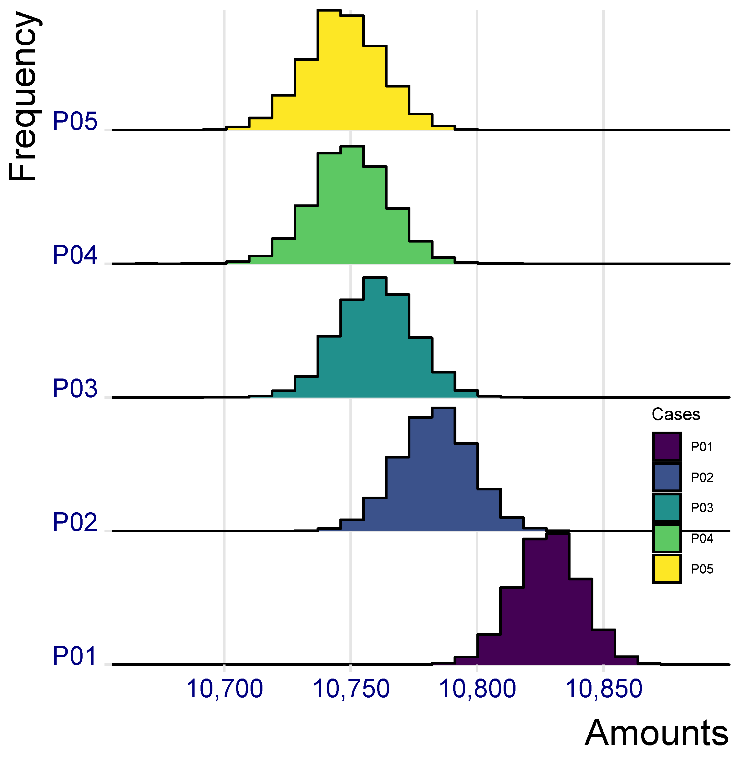
Empirical distributions at times 5 and 10 of the portfolio payout, that is, empirical distributions of $X\left(5\right)$ and $X\left(10\right)$, are sketched in Figure 3 and Figure 4, where the three portfolios are denoted by $\mathrm{P}01$, $\mathrm{P}02$ and $\mathrm{P}03$, respectively.

7.1.2. Cases 1.4

To assess the impact of a possible cannibalization effect, we consider three portfolios with the following sub-portfolio sizes:

$$\begin{array}{cc}\hfill n_1& =\mathrm{10,000}-\frac{n_2}{2}\hfill \\ \hfill n_2& =500,800,1000\hfill \\ \hfill n_3& =\frac{n_2}{2}=250,400,500\hfill \end{array}$$

As previously noted, to represent an improvement in mortality in the standard annuity sub-portfolio, we assume $M_1=91$ (instead of $M_1=90$). Empirical distributions of the portfolio payout $X\left(5\right)$ and $X\left(10\right)$ are sketched in Figure 5 and Figure 6, respectively, where the three portolios are denoted by $\mathrm{P}01$, $\mathrm{P}02$ and $\mathrm{P}03$.

7.1.3. Some Comments

Results are self-explanatory, and in line with the findings in the deterministic setting: the larger the (initial) number of enhanced annuities in Cases 1.1, the higher the dispersion in the annual payouts. The same effect is, of course, witnessed by the distributions of payouts in Cases 1.4, where presence of both enhanced annuities and impaired annuities is assumed.

7.2. Impact of the Lifetime Distribution

To assess the impact of uncertainty in biometric assumptions, we only analyze the Cases 2.1 considered in Section 6.2.

7.2.1. Cases 2.1

We consider a portfolio only consisting of standard annuities and enhanced annuities, with given sub-portfolio sizes. Hence:

$$\begin{array}{cc}\hfill n_1& =\mathrm{10,000}\hfill \\ \hfill n_2& =1000\hfill \\ \hfill n_3& =0\hfill \end{array}$$

We analyze the impact of diverse assumptions on the dispersion of lifetimes. Then:

$$D_2=4,6,8,10,12$$

(while keeping $D_1=5$). Empirical distributions of the portfolio payout $X\left(5\right)$ and $X\left(10\right)$ are sketched in Figure 7 and Figure 8, where the portfolios are respectively denoted by $\mathrm{P}01,\dots ,\mathrm{P}05$.

7.2.2. Some Comments

These results are self-evident: a larger dispersion in the lifetime distribution of annuitants with enhanced annuity implies a larger dispersion in the total portfolio payout (compare, in particular, distributions in portfolio $\mathrm{P}05$ and $\mathrm{P}01$. Moreover, for all the portfolios, dispersions increase with time (compare the distributions in Figure 7 to the ones in Figure 8).

7.3. Meeting the Annual Payouts

Appropriate resources must be assigned to the portfolio in order to meet the annual payouts with a high probability. Diverse criteria can be adopted to quantify the above resources which, whatever the criterion adopted, will partly be provided by single premiums cashed at policies issued (via decumulation of the portfolio reserve) and partly by shareholders’ capital allocated to the portfolio. In what follows, we focus on the annual total amount of resources needed, disregarding the funding source.

7.3.1. The Percentile Principle

Referring to a generic portfolio and the relevant cash flows, we recall that $X_1\left(t\right)$, $X_2\left(t\right)$, $X_3\left(t\right)$ denote the random payouts at time t, related to standard annuities, enhanced annuities and impaired annuities, respectively (see Section 5.4), and:

$$X\left(t\right)=X_1\left(t\right)+X_2\left(t\right)+X_3\left(t\right)$$

(15)

denotes the portfolio total payout at time t.

We adopt the percentile principle. Hence, we have to find, for $t=1,2,\dots$, the amount $A\left(t\right)$ such that:

$$Pr\left[X\right(t)>A(t\left)\right]=\epsilon$$

(16)

where $\epsilon$ denotes an assigned (small) probability; hence, $1-\epsilon$ can be interpreted as the “adequacy” level.

A more detailed analysis could be performed by separately addressing the risk profile of each sub-portfolio, thus calculating, for $k=1,2,3$ and $t=1,2,\dots$ the quantities $A_k\left(t\right)$ such that:

$$Pr[X_k\left(t\right)>A_k\left(t\right)]={\epsilon }_k$$

(17)

However, we only focus on the overall requirement (16), which clearly takes into account the pooling effect.

7.3.2. Numerical Results

We consider four portfolios with the structures defined in

Table 9. Portfolio structures.

Portfolio	${\mathit{n}}_1$	${\mathit{n}}_2$	${\mathit{n}}_3$
P01	10,000	0	0
P02	10,000	1000	0
P03	10,000	0	500
P04	10,000	1000	500

.

This way, we can analyze the risk profile of a “traditional” portfolio only consisting of standard annuities (P01), a portfolio including standard annuities and enhanced annuities (P02) or standard annuities and impaired annuities (P03) and finally a portfolio including both types of special-rate annuities (P04).

Values of the parameters $M_k$ and $D_k$ for standard life annuities ($k=1$), enhanced annuities ($k=2$) and impaired annuities ($k=3$), respectively, are as specified in Table 1.

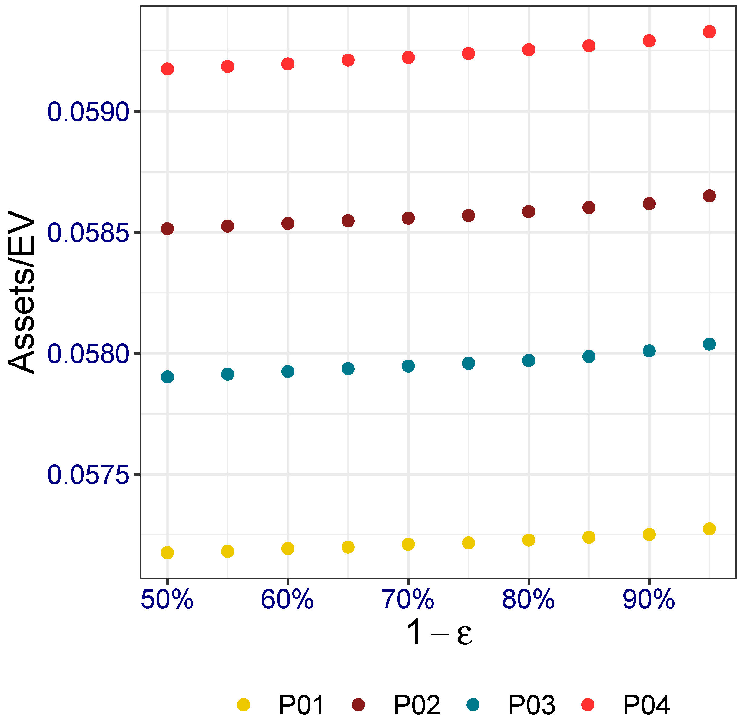
Asset requirements (at a given time t), in terms of ratios ${\displaystyle \frac{\mathrm{Assets}}{EV}}$, where $EV$ denotes the expected value of the total payout, are plotted in Figure 9, Figure 10 and Figure 11 against the probability $1-\epsilon$.

7.3.3. Some Comments

Results in terms of assets requirements are also encouraging. We note that the range of values, expressed by the ratio between assets required and expected values of total payout, corresponding to the various portfolio structures are very limited, whatever the adequacy level chosen. A higher sensitivity with respect to the adequacy level $1-\epsilon$ can be observed in particular for $t=10$, because of a dispersion of the numbers of survivors and hence of the total payouts, which increases with time.

We note that the portfolio structure of course evolves over time and, notably, the share of standard annuities progressively increases because of longer lifetimes of standard annuitants. Increasing shares of standard life annuities (characterized, according to a reasonable assumption, by a variance lower than that of special-rate annuities) imply a lower riskiness in the (total) annuity portfolio. In terms of the ratio Assets/EV, this effect appears in particular when comparing the requirements (according to each probability $1-\epsilon$) represented in Figure 9, Figure 10 and Figure 11.

8. Concluding Remarks

By offering special-rate life annuities, on the one hand, a higher premium income can be expected, while on the other hand, a higher variability of the total portfolio payout will follow because of both the larger size and the specific higher variability of payouts related to special-rate annuities.

The analysis, in quantitative terms, of the “balance” between the two aspects (that is, higher risk and higher premium income) has been the aim of this research. A number of numerical evaluations have been performed by adopting both a deterministic approach and a stochastic one as well. Diverse hypotheses on lifetime distributions have been assumed, and various portfolio sizes and structures (in terms of numbers of standard, enhanced and impaired annuities) have been considered.

It is worth noting that, whatever the choice of the parameter values for the Gompertz law, the mortality model is deterministic, in the sense that no uncertainty in future mortality trend is accounted for. In this context, it is reasonable to assume independence among the individual lifetimes. An interesting extension of our simple model should allow for uncertainty in mortality trends via an appropriate stochastic mortality model. Then, correlation among lifetimes would follow, so that independence assumption would be replaced by conditional independence. Moreover, diverse trends and diverse degrees of uncertainty could be considered for the various special-rate annuities by taking into account possible improvements in medical treatments, surgery, etc.

Special attention should be placed on the “cannibalization” effect. First, a reduction in the size of the standard annuity sub-portfolio may occur, provided that some applicants can be eligible to special-rate annuities. A lower average mortality in the standard sub-portfolio then follows (as noted in Section 6.1.5), leading to a (reasonable) increase in standard annuity premiums. This might in turn impact the demand of standard life annuities (even beyond the reduction mentioned above).

A further aspect that is interesting to investigate is the impact on the insurer’s liabilities (and, notably, on the portfolio risk profile) of an incorrect allocation of individual risks to the various rating classes. Because of the presence of unobservable risk factors, a misspecification of the rating class is always possible. This would result in an unfair annuity rate applied to some individuals and then in an increased (or reduced) probability of loss for the insurer. In this regard, the research task should concern, in particular, the modeling of the incorrect specification of the rating class.

The results we have obtained of course depend on assumptions (notably, regarding both the portfolio structure, the mortality model and the relevant parameters). Nevertheless, the broad range of assumptions regarding both the portfolio structure and the lifetime distributions has allowed us to perform an effective sensitivity analysis, whose interesting achievements witness the possibility of extending the life annuity business without taking huge amounts of risk. Hence, the creation of values for customers (and an increase in the insurer’s market share) can be pursued without a significant worsening of the company’s risk profile.