
A New Class of Counting Distributions Embedded in the Lee–Carter Model for Mortality Projections: A Bayesian Approach

1
Sakhnin Academic College, Galilee St. 100, Sakhnin 30810, Israel
2
Faculty of Industrial Engineering and Technology Management, HIT—Holon Institute of Technology, 52 Golomb Street, Holon 5810201, Israel
3
Actuarial Research Center, University of Haifa, 199 Aba Khoushy Ave. Mount Carmel, Haifa 3498838, Israel
*
Author to whom correspondence should be addressed.
Risks 2022, 10(6), 111; https://doi.org/10.3390/risks10060111
Submission received: 24 March 2022
/
Revised: 13 May 2022
/
Accepted: 18 May 2022
/
Published: 27 May 2022
(This article belongs to the Special Issue Actuarial Mathematics and Risk Management)
Abstract
:The Lee–Carter model, the dominant mortality projection modeling in the literature, was criticized for its homoscedastic error assumption. This was corrected in extensions to the model based on the assumption that the number of deaths follows Poisson or negative binomial distributions. We propose a new class of families of counting distributions, namely, the ABM class, which belongs to a wider class of natural exponential families. This class is characterized by its variance functions and contains the Poisson and the negative binomial distributions as special cases, offering an infinite class of additional counting distributions to be considered. We are guided by the principle that the choice of distribution should be made from a pool of distributions as large as possible. To this end, and following a data mining approach, a training set of historical mortality data of the population could be modeled using the ABM’s rich choice of distributions, and the chosen distribution should be the one that proved to offer superior projection results on a test set of mortality data. As an alternative to parameter estimation via the singular value decomposition used in the classical Lee–Carter model, we adopted Bayesian estimation, harnessing the Markov Chain Monte Carlo methodology. A numerical study demonstrates that when fitting mortality data using this new class of distributions, while traditional distributions may provide desirable projections for some populations, for others, alternative distributions within the ABM class can potentially produce superior results for the entire population or particular age groups, such as the oldest-old.
1. Introduction
The seminal paper by Lee and Carter (1992) (LC) introduced a model which is one of the most well-known and widely applied models for forecasting mortality rates. Within this model, the time series of the log mortality rates, of each age is described by an age-specific intercept plus a common trend for all age groups multiplied by an age-specific coefficient
The error term is assumed to be distributed with a mean 0 and variance , reflecting influences missed by the model. The age and time-specific mortality rate is calculated as , where denotes the number of deaths in a population at age and at time , and is the exposure to the risk of death. To ensure the identifiably of model parameters, constraints are imposed such that the sum of over age is 1 and the sum of over time is 0. To forecast mortality rates into the future, a simple random walk with drift is proposed for :
The homoscedastic error assumption of the Lee–Carter model was criticized for its limiting impact on predictions (Brouhns et al. 2002; Danesi et al. 2015; Idrizi 2018). This led to the introduction of the Poisson log-bilinear LC-type model (Brouhns et al. 2002), which, in contrast, is intrinsically heteroscedastic, namely:
Here, the number of dead is directly modelled by a Poisson distribution, whose parameter is estimated by maximum likelihood estimation (MLE). This alternative approach gained momentum and alternative discrete distributions were proposed. In particular, a binomial distribution was proposed by Wang and Lu (2005) and a negative binomial distribution was suggested by Delwarde et al. (2007) and Renshaw and Haberman (2008). See Azman and Pathmanathan (2022) for further discussion of these distributions within the GLM framework.
The Lee–Carter model has been widely used for many purposes (Shair et al. 2018), such as forecasting mortality reduction factors, assessing the adequacy of retirement income, population projections and the projection of mortality trends for the oldest-old (older than 80, and in some sources 85). This age group is of considerable interest for policymakers as it is destined to grow as a proportion of the entire population and can outstrip existing infrastructures’ capacity (Buettner 2002). This is a fairly recent phenomenon. In Canada, for instance (Legare et al. 2015), the 21st century brought about the most significant gain in life expectancy at age 85 (7.79% for women and 9.93% for men). Clearly, policies need to be devised that can meet people’s special needs in what is called the fourth age Baltes and Smith (2003), and accurate mortality projection for this age group is a must. We shall, therefore, focus on the adequacy of potential underlying discrete distribution functions to produce accurate mortality projections using the Lee–Carter model for this age group. This will be discussed in Section 4.
In essence, while the above-cited papers relied on popular and commonly used discrete distributions, one cannot say that one particular distribution is universally superior. Indeed, it is entirely plausible to assume that there is a winning distribution for any given population or even for a specific population at a certain age range. Ideally, one should consider a rich class of family of counting distributions, much richer than the two already suggested, and use the data to pick the most suitable distribution for the population under study. This paper proposes an infinitely countable set of families of counting distributions, where the Poisson, negative binomial and Abel families of distributions are special cases. Our aim is to study this family, incorporate it into the framework of the LC model and use real data to seek the most suitable distribution for mortality projection. While there is little doubt that the distributions discussed above could prove adequate for specific populations or age groups, other distributions within the suggested family could have the upper hand.
The paper is organized as follows. Section 2 presents the new class of counting distributions. Section 3 is devoted to the new class and its Bayesian framework. Section 4 (divided into Section 4.1: Methods and Section 4.2: Results) reports a numerical study in which superior members of this class are chosen for mortality projections of the oldest-old in three populations. Finally, Section 5 offers a discussion.
2. A New Class of Counting Distributions on the Set of Nonnegative Integers
The new class of families of counting distributions on the non-negative integers belongs to a wider class of natural exponential families (NEFs), characterized by their variance functions (VFs). In order to comprehend this class we decompose this section into subsections. We first present some preliminaries on NEFs and their associated VFs. We then introduce a class of NEFs having polynomial structure and then suggest the new class of families of counting distributions, named ABM, first introduced by Awad et al. (2016), where the class was defined and its usefulness for mortality projections was preliminary sketched. Furthermore, such a class has been investigated by Bar-Lev and Ridder (2021a, 2021b) from a classical frequency approach and has shown superiority with respect to various metrics or goodness-of-fit tests for different count datasets (for further details see item 6 in Section 2.3).
2.1. NEFs—Some Preliminaries
The following preliminaries are mainly taken from Letac and Mora (1990) and are briefly presented here for completeness.
Let be a non-Dirac positive Radon measure on , and its Laplace transform. Assuming that , then the NEF generated by is defined by the probability distributions
where , the cumulant transform of , is strictly convex and real analytic on . If represents a r.v. having distribution of the form given in (1) then the expectation and variance of are given, respectively, by and where is strictly monotone and thus its inverse, say, is well defined. The set M of all means of (1) is called the mean parameter space of . The variance of can be expressed in terms of m by . The pair is called the VF of and it uniquely determines within the class of NEFs. For example, and are, respectively, the VFs of the Poisson and exponential NEFs and are uniquely determined by them.
2.2. The Mean Value Parametrization of NEFs
As indicated above, the VF of an NEF uniquely determines F within the class of NEFs. Let be a given VF of an NEF generated by . Then, simple calculations show both and the cumulant transform of can be expressed in terms of m as:
where one needs to determine the constants and so that , constitutes a probability distribution (not an easy task). Accordingly, a mean value parametrization of an NEF generated by a measure is given by:
Such a representation of is more natural as it is expressed in terms of the mean m rather than a somewhat artificial parameter . A comprehensive description of NEFs in terms of their mean value representation is reviewed in Bar-Lev and Kokonendji (2017).
Remark 1.
The task of computing the constants and is not simple and might be rather cumbersome. However, from a Bayesian perspective, when (3) is used as a prior distribution on m, then in the calculation of the respective posterior distribution, such constants are cancelled out (as the likelihood function is the only relevant component). As this paper is concerned with a Bayesian framework, one can assume without any loss of generality that . Henceforth, we indeed assume so.
2.3. Polynomial VFs of Counting NEFs Supported on the Set of Nonnegative Integers
The innovative and breakthrough Proposition 4.4 of Letac and Mora (1990, p. 13) provided conditions under which a given VF is associated with a counting NEF F supported on the set of non-negative integers , i.e., where all members of F are composed of counting distributions on . They provided general examples of two classes of VFs which fulfill the premises of their Proposition 4.4 and thus their associated NEFs’ distributions are supported on the non-negative integers. One of these two classes has the form:
They proved that such VFs constitute counting NEFs supported on namely, counting distributions with non-negative integer support. Moreover, their Proposition 4.4 enables to compute (at least theoretically and numerically) the corresponding measure (we skip details as they are irrelevant for our Bayesian framework analysis). Note that the two special cases of (4) with and correspond, respectively, to the Poisson and negative binomial NEFs. However, the general setting (4) for does not allow an explicit calculation of and in (2), implying that the mean value parametrization of the corresponding NEFs in the form (3) is not explicitly expressible in terms of m and thus becomes useless for any practical consideration.
2.4. A New Class of Polynomial VFs—The ABM NEFs
As we already noted, the fact that a given pair is known to be a VF of some NEF does not necessarily enable the construction of the corresponding mean value parameterization (3), as in most cases the integrals for and in (2) are not explicitly expressible analytically in closed forms, and indeed, this is the situation for the class (4) in its general form. Consequently, one needs to search for subclasses of (4) for which the integrals in (2) can be computed explicitly. One such special subclass takes the above point into consideration. Indeed, by taking in (4) the special case where
and denoting
we obtain a subclass of (4) with VFs with the form:
As (5) is a subclass of (4) and (4) satisfies the premises of Proposition 4.4 of Letac and Mora (1990) it follows that the subclass (5) are VFs associated with counting NEFs supported on the non-negative integers.
The subclass of VFs in (5) (hereafter called the ABM class) was first introduced by Awad et al. (2016) who showed that the corresponding and (calculated from (2)) have, as opposed to the general form in (4), the following closed forms (the exact proof details appear in Bar-Lev and Kokonendji 2017):
and
Thus, its mean value parametrization is given by the probability distribution:
where hereafter we denote this probability distribution by where is a positive real number and is a non-negative integer. (For a classical frequency approach, the constants and have been computed by Bar-Lev and Ridder 2021b). However, as noted above, for a Bayesian framework they are cancelled out when computing the posterior distribution and thus can be taken to be without any loss of generality).
Note that the ABM class of VFs , or alternatively, the corresponding class of NEFs is composed of an infinitely countable set of families of counting NEFs supported on the non-negative integers. As special cases, this class contains the Poisson NEF (), the negative binomial NEF ( and the Abel NEF (), (c.f., Letac and Mora 1990, p. 31; Bar-Lev and Ridder 2019, for applications to car accident claims of a Swedish insurance company dataset).
Summarizing, this ABM NEF has the following features:
- It is a class of counting distributions supported on the non-negative integers;
- It is overdispersed as ;
- It allows a mean value parameterization in a closed form;
- It is infinitely divisible, which allows the construction of an exponential dispersion model (EDM) with dispersion parameter space equal to . EDMs are used to describe the error distribution in generalized linear models (see Jorgensen 1987, 1997);
- is an unknown parameter to be estimated (see next section). is a parameter governing the particular model within the ABM class and is considered to be a decision variable (note that different values of determine different ABM NEFs). Accordingly, for given national datasets (i.e., those of US, Ireland and Ukraine), the goal will be to locate that value of , which minimizes a respective RMSE (see in the sequel). However, due to the rather cumbersome and intractable structure of the ABM probabilities (or likelihood) in (6) and the fact that the larger the , the larger the number of elements in the summands appearing in (6), no analytic solution for an optimal is feasible at all for achieving such a goal. Consequently, only numerical search algorithms are plausible. The search starts with (the Poisson NEF), (the negative binomial NEF), (the Abel NEF) and so on;
- As already noted, the ABM class is composed of infinitely countable set of families of counting NEFs supported on the non-negative integers and thus can also be used to model real datasets by employing the classical frequency approach (and not only Bayesian). Indeed, the ABM class has been compared in Bar-Lev and Ridder (2021a, 2021b) with other common counting probability models (such as Poisson-inverse Gaussian distribution, new logarithmic distribution, an exponentiated discrete Lindley distribution) for various real count datasets stemming from automobile insurance claims, marketing, biometry, health, and social sciences (none of which is related to mortality projections). Members of the ABM counting class have shown superiority with respect to various metrics for goodness-of-fit tests (chi-squared test, Akaike information criterion (AIC), root-mean-square error (RMSE) and Kullback–Leibler divergence (KL)), and provided a much better fit for each of the datasets considered (more details can be found in Bar-Lev and Ridder 2021b).
3. ABM Based LC Model and its Bayesian Framework
As an alternative to parameter estimation via the singular value decomposition used in the classical LC model or the MLE in the cases discussed above, we adopt the Bayesian approach which offers advantages succinctly expressed in Antonio et al. (2015): a. The calibration and forecast steps are combined, which leads to more consistent estimates of the period effects; b. The Bayesian approach provides a natural framework for incorporating parameter uncertainty in mortality forecasts, which is relevant—for example—in the new insurance regulatory framework of Solvency II. The Bayesian approach allows adequate handling of small populations and missing data. Like Czado et al. (2005) and Pedroza (2006), we harness the power of the Markov Chain Monte Carlo (MCMC) methodology to estimate the model parameters and execute mortality projection. We note that the interest in Bayesian solutions in the context of mortality projections has recently gained momentum (Ellison et al. 2020; Graziani 2020; Hilton et al. 2019; Hunt and Blake 2020; Kogure et al. 2019; Liu et al. 2020; Njenga and Sherris 2020; Wong et al. 2018).
Suppose the number of deaths in a population at age x and time t is distributed as follow:
where
Bayesian estimation of the unknown parameters and are based on the joint posterior distribution function of and given , when . The first step in the Bayesian estimation is to determine the prior probability functions for these parameters.
The prior distribution for and
Let and let and hence . we assume and . The hyper-parameters and are arbitrary initial values.
The prior distribution for
We assume ∀ x, where . The hyper-parameters are arbitrary initial values.
The prior distribution for
We suppose that the prior distribution of ∀ x, where . The hyper-parameters and are arbitrary initial values.
The prior distribution for
We let . The hyper-parameters are arbitrary initial values.
MH (Metropolis–Hastings) Algorithm for Estimating the Parameters and
Suppose the are independent random variables, which are distributed as (6) and is the joint prior distribution of the unknown parameters . Then, the posterior distribution of given all available data and can be represented as follows:
See Appendix A for the marginal posterior distributions of and . We now describe the estimation of and using the MH, conditioned on the data and all other parameters at their respective iterations. The superscript denotes the iteration number of the parameter of interest.
Estimation of using the MH algorithm
Let the marginal posterior distribution of be . The estimation of is achieved by the following steps, where.
- Draw from the proposal density function , such that is assumed known;
- Calculate the following probability:where
- Draw a value u from uniform probability function in range and decide in accordance with the following formula:
- Going over all values of t, we have:
- Transforming and to assure identifiably:where
- Repeat steps 1 to 5.
Estimation of using MH algorithm
Let the marginal posterior distribution of be The estimation of is achieved by the following steps.
- Draw from the proposal density function , such that is assumed to be known;
- Calculate the following probability:where
- Draw a value u from uniform probability function in range and decide in accordance with the following formula:
- Going over all values of x, we have:
- Transforming and to assure identifiably:where
- Repeat steps 1 to 5.
Estimation of using MH algorithm
Let the marginal posterior distribution of be The estimation of is achieved by the following steps;
- Draw from the proposal density function , such that is assumed known;
- Calculate the following probability:where
- Draw a value u from uniform probability function in range and decide in accordance with the following formula:
- Receiving in th iteration as follows:
- Repeat steps 1 to 4.
Estimation of using MH algorithm
Let the marginal posterior distribution of be , proportional to the product of the likelihood (6) and the gamma prior distribution of . The estimation of is achieved by the following steps;
- Draw from the probability function , such that and are hyperparameters and are assumed known;
- Calculate the following probability:
- Draw a value u from uniform probability function in range and decide in accordance with the following formula:
- Then receiving in th iteration;
- Repeat steps 1 to 4.
Estimation of and using the Gibbs sampler
The Gibbs sampler can be used for estimating and since the marginal posterior distribution of these parameters can be written explicitly (See: (Czado et al. 2005)). The following are the marginal posterior sampling distributions of each of these parameters, conditioned on the data and all other parameters at their respective iterations.
1. Sampling :
The posterior probability function of the parameter , is presented as follows:
The prior probability function of the parameter is , and the hyper-parameters and are set by the user, hence the posterior probability function of the parameter is:
2. Sampling :
The posterior probability function of the parameter is presented as follows:
The prior probability function of the parameter such that , and the hyper-parameters and are set by the user, so the posterior probability function of the parameter is:
where
3. Sampling :
The posterior probability function of the parameter is presented as follows:
The prior probability function of the parameter such that , and the hyper-parameters and are set by the user, so the posterior probability function of the parameter is:
4. Sampling :
The posterior probability function of the parameter , is presented as follows:
The prior probability function of the parameter such that , and the hyper-parameters and are set by the user, so the posterior probability function of the parameter is:
4. Numerical Experiment
4.1. Methods
To test the adequacy of the ABM class, we analyzed mortality data of men in Ireland, Ukraine and the USA, downloaded from the database of Human Mortality Database (https://www.mortality.org accessed on 8 March 2013). The data contain the number of dead and the size of the population exposed to risk by age and year; Ireland’s and the USA’s data are for 1950–2007, and Ukraine’s data are for 1959–2009. This analysis aims to examine sixteen models within the ABM class, , with a particular emphasis on forecasting the mortality of the oldest-old (see below an argumentation for the restriction of the values of to ). These models also include the Poisson and negative binomial models which feature widely in the literature, for which and , respectively. Adopting a data mining approach, the models were fitted using training sets and were examined using test sets. The training sets contained data up to 2000 and the test sets, aimed at monitoring the quality of predictions, contained data from 2001 to 2007 for Ireland and the USA, and from 2001 to 2009 for Ukraine. Predictions are carried out with the estimated parameters, where model performance (using the test sets) was checked using the root of the mean squared errors (RMSE), which was calculated in two ways:
- Predicting mortality rates by age. In other words, after model parameters were estimated, mortality rates were predicted for a given age across years. For instance, predicting mortality rates for those age 70 was carried out over the years beyond 2000;
- Predicting mortality rates by cohort. In other words, after model parameters were estimated, mortality rates were predicted for a cohort that was at a particular age at the beginning of the test period. For example, predicted mortality rates in 2001–2007 for a cohort aged 70 in 2001.
For every member of the ABM class (controlled by ), the Markov chains used to obtain posterior distributions/parameter estimates comprised 4000 iterations with the first 1000 considered a burn-in period. Convergence was established using graphical means and a sensitivity analysis ascertained that the choice of arbitrary initial hyper-parameters did not affect the final outcomes. We report the outcomes for the Poisson distribution ( and the negative binomial distribution (. In addition, we examined the ABM members for which We limited our reporting to since, for the data under study, increasing beyond 15 (our study explored all models up to did not alter our findings of the optimal for varying ages and resulted in much larger RMSE than those found up to = 15. In practice, we analyzed all 16 models within the range and, for each, we estimated as well as all other unknown parameters. Finally, we reported graphically the RMSE for the Poisson, negative binomial and for the ABM member which produced the minimal RMSE for various ages.
4.2. Results
Figure 1a,b shows Ireland’s mortality projections by age and cohort, respectively. A superior model for an age range is the one which produced the smallest RMSE. It is evident that the Poisson performs best for most ages above 70, with the negative binomial lagging behind. However, at a very old age, the Poisson diverges and the best ABM member to be chosen instead is A similar result is shown for the USA (Figure 2a,b), except that the best ABM for the very old is . A different picture emerges when we focus on Ukraine’s mortality projections by age and cohort (Figure 3a,b, respectively). While the Poisson and negative binomial perform well (with Poisson being better), for ages above 96 (by cohort) or 104 (by age), the negative binomial drifts away, leaving to be the winner of the ABM class. Clearly, the recommended projection policy for Ukraine is to use the Poisson for most ages but to rely on for very old ages. Naturally, other countries with their specific national datasets may yield different ABM models (i.e., different ’s) for mortality projections.
5. Discussion
Several extensions to the LC model assume that the number of deaths is distributed Poisson or negative binomial. These distributions have offered adequate mortality projections in several populations reported in the literature. It is not implausible that cases where these two failed were not reported. Rather than deciding a priori to choose a particular distribution, we aimed to enrich the LC model by allowing a richer pool of candidate distributions. The chosen distribution would be the one providing the best projection for the population and age range under study. To achieve this goal, we proposed a new class of counting distributions on the non-negative integers, the ABM class, which belongs to a wider class of natural exponential families characterized by their variance functions. This class includes the Poisson and negative binomial distributions which are included in an infinitely countable set of additional members. A data mining approach was adopted whereby the model is fitted using a training set and tested using a test set with the RMSE used to pick the winning model. As an alternative to parameter estimation via the singular value decomposition (SVD) used in the classical LC model, we adopted Bayesian estimation, harnessing the Markov Chain Monte Carlo (MCMC) methodology. While we do not suggest that MCMC is superior to SVD (for a comparison of the two, see Ichikawa et al. 2021), we still promote the former since the Bayesian framework frees us from the burden of calculating the normalizing constant of the ABM. This is indeed a great plus, even though running the MCMC requires more computer time for the mid-size databases of the kind used for national mortality projections. We note, however, that the use of MCMC is rather costly and might fail if the dataset is huge. So, perhaps other Bayesian techniques such as Variational Bayes can be more helpful. However, employing such a suggestion is beyond the scope of this paper. We examined ABM models for three countries and established that, for the countries examined, the commonly adopted Poisson distribution is justified except for a very old age for which an alternative member of the ABM class offers better projection. We do not claim that to suggest a superior model. When deciding on an underlying model, one can adopt as an example the Poisson model or the negative binomial model. Rather than adopting a model, we suggest adopting a class of models (the ABM) comprising the Poisson, negative binomial, and numerous other counting distributions. The superiority of this approach lies in the ability to choose a model amongst candidate models. Since no one single model necessarily fits every population and every age group well, the ABM class could allow picking, as an example, the Poisson for members of the population aged under 50, the negative binomial for those aged 50 to 80, and another member of the class to the oldest-old. The suggested criteria for preferring one member of the class over another is the mean squared projection errors (RMSE). This advantage is gained at the cost of additional complexity, which is justified given the financial benefits associated with more accurate modeling. We conclude that it is no longer appropriate to assume a single distribution for the whole process of mortality projection. Instead, for every country and every relevant range of ages, a desirable approach is to pick a member of the ABM class that provides the best mortality projection. In the numerical study reported here, neither the Poisson nor the negative binomial distributions adequately serve the very oldest-old and superior alternatives are within reach in the suggested novel ABM class of distributions.
Author Contributions
Conceptualization, Y.A., S.K.B.-L. and U.M.; methodology, Y.A., S.K.B.-L. and U.M.; software, Y.A.; validation, Y.A., S.K.B.-L. and U.M.; formal analysis, Y.A., S.K.B.-L. and U.M.; investigation, Y.A., S.K.B.-L. and U.M.; resources, Y.A., S.K.B.-L. and U.M.; data curation, Y.A.and U.M.; writing—original draft preparation, Y.A., S.K.B.-L. and U.M.; writing—review and editing, Y.A., S.K.B.-L. and U.M.; visualization, Y.A., S.K.B.-L. and U.M. All authors have read and agreed to the published version of the manuscript.
Funding
This research received no external funding.
Institutional Review Board Statement
Not applicable.
Informed Consent Statement
Not applicable.
Data Availability Statement
Publicly available datasets were analyzed in this study. This data can be found here: the database of Human Mortality Database (https://www.mortality.org access on 8 March 2013).
Conflicts of Interest
The authors declare no conflict of interest.
Appendix A
Appendix A.1
The marginal posterior probability function of the time index is
where
For the remaining expressions we distinguish between three cases:
- For , the marginal posterior probability function of the time index is:where
- For , the marginal posterior probability function of the time index is:where
- For , the marginal posterior probability function of the time index is:where
Appendix A.2
The marginal posterior probability function of is
where
and
Appendix A.3
The marginal posterior probability function of is
where
and
References
- Antonio, Katrien, Anastasios Bardoutsos, and Wilbert Ouburg. 2015. Bayesian Poisson log-bilinear models for mortality projections with multiple populations. Eur. Actuar. J. 5: 245–281. [Google Scholar] [CrossRef]
- Awad, Yaser, Shaul K. Bar-Lev, and Udi Makov. 2016. A New Class Counting Distributions Embedded in the Lee–Carter Model for Mortality Projections: A Bayesian Approach. Technical Report No. 146. Israel: Actuarial Research Center, University of Haifa. [Google Scholar]
- Azman, Shafiqah, and Dharini Pathmanathan. 2020. The GLM framework of the Lee–Carter model: A multi-country study. Journal of Applied Statistics 49: 752–63. [Google Scholar] [CrossRef]
- Baltes, B. Paul, and Jacqui Smith. 2003. New frontiers in the future of aging: From successful aging of the young old to the dilemmas of the fourth age. Gerontology 49: 123–35. [Google Scholar] [CrossRef] [PubMed]
- Bar-Lev, K. Shaul, and Ad Ridder. 2019. Monte Carlo methods for insurance risk computation. International Journal of Statistics and Probability 8: 54–74. [Google Scholar] [CrossRef]
- Bar-Lev, K. Shaul, and Ad Ridder. 2021a. Exponential dispersion models for overdispersed zero-inflated count data. Communications in Statistics-Simulation and Computation. Available online: https://doi.org/10.1080/03610918.2021.1934020 (accessed on 10 August 2021).
- Bar-Lev, K. Shaul, and Ad Ridder. 2021b. New exponential dispersion models for count data—The ABM and LM classes. ESAIM: Probability and Statistics 25: 31–52. [Google Scholar] [CrossRef]
- Bar-Lev, K. Shaul, and Clestin C. Kokonendji. 2017. On the mean value parametrization of natural exponential families—A revisited review. Mathematical Methods of Statistics 26: 159–75. [Google Scholar] [CrossRef]
- Brouhns, Natacha, Michel Denuit, and Jeroen K. Vermunt. 2002. A Poisson log-bilinear regression approach to the construction of project life-table. Insurance: Mathematics and Economics 31: 373–93. [Google Scholar]
- Buettner, Thomas. 2002. Approaches and experiences in projecting mortality patterns for the oldest-old. North American Actuarial Journal 6: 14–29. [Google Scholar] [CrossRef]
- Czado, Claudia, Antoine Delwarde, and Michel Denuit. 2005. Bayesian Poisson log-bilinear mortality projections. Insurance: Mathematics and Economics 36: 260–84. [Google Scholar] [CrossRef] [Green Version]
- Danesi, L. Ivan, Steven Haberman, and Pietro Millossovich. 2015. Forecasting mortality in subpopulations using Lee—Carter type models: A comparison. Insurance: Mathematics and Economics 62: 151–61. [Google Scholar] [CrossRef]
- Delwarde, Antoine, Michel Denuit, and Christian Partrat. 2007. Negative binomial version of the Lee–Carter model for mortality forecasting. Applied Stochastic Models in Business and Industry 23: 385–401. [Google Scholar] [CrossRef]
- Ellison, Joanne, Erengul Dodd, and Jonathan J. Forster. 2020. Forecasting of cohort fertility under a hierarchical Bayesian approach. Journal of the Royal Statistical Society: Series A (Statistics in Society) 183: 829–56. [Google Scholar] [CrossRef]
- Graziani, Rebecca. 2020. Stochastic Population Forecasting: A Bayesian Approach Based on Evaluation by Experts. Developments in Demographic Forecasting 49: 21–42. [Google Scholar]
- Hilton, Jason, Erengul Dodd, Jonathan J. Forster, and Peter W. F. Smith. 2019. Projecting UK mortality by using Bayesian generalized additive models. Journal of the Royal Statistical Society: Series C (Applied Statistics) 68: 29–49. [Google Scholar] [CrossRef]
- Hunt, Andrew, and David Blake. 2020. A Bayesian Approach to Modeling and Projecting Cohort Effects. North American Actuarial Journal 25: S235–S254. [Google Scholar] [CrossRef]
- Ichikawa, Shota, Hiroyuki Yamamoto, and Takumi Morita. 2021. Comparison of a Bayesian estimation algorithm and singular value decomposition algorithms for 80-detector row CT perfusion in patients with acute ischemic stroke. La Radiologia Medica 126: 795–803. [Google Scholar] [CrossRef]
- Idrizi, Olgerta. 2018. The Heteroscedasticity Impact on Actuarial Science: Lee Carter Error Simulation. European Journal of Engineering and Formal Sciences 1: 1–12. [Google Scholar] [CrossRef]
- Jorgensen, Bent. 1987. Exponential dispersion models (with discussion). Journal of the Royal Statistical Society, Series B 49: 127–62. [Google Scholar]
- Jorgensen, Bent. 1997. The Theory of Exponential Dispersion Models. Monographs on Statistics and Probability 76. London: Chapman and Hall. [Google Scholar]
- Kogure, Atsuyuki, Takahiro Fushimi, and Shinichi Kamiya. 2019. Mortality Forecasts for Long-Term Care Subpopulations with Longevity Risk: A Bayesian Approach. North American Actuarial Journal 25: S534–44. [Google Scholar] [CrossRef]
- Lee, D. Ronald, and Lawrence R. Carter. 1992. Modelling and forecasting the time series of US mortality. Journal of the American Statistical Association 87: 659–71. [Google Scholar]
- Légaré, Jacques, Yann Décarie, Kim Deslandes, and Yves Carrière. 2015. Canada’s oldest old: A population group which is fast growing, poorly apprehended and at risk from lack of appropriate services. Population Change and Lifecourse Strategic Knowledge Cluster Discussion Paper Series/Un Réseau Stratégique de Connaissances Changements de Population et Parcours de vie Document de Travail 3: 1. Available online: https://ir.lib.uwo.ca/pclc/vol3/iss2/1 (accessed on 1 April 2021).
- Letac, Gerard, and Marianne Mora. 1990. Natural real exponential families with cubic variance functions. Annals of Statistics 18: 1–37. [Google Scholar] [CrossRef]
- Liu, Zhen, Xiaoqian Sun, Leping Liu, and Yu-Bo Wang. 2020. Bayesian Poisson Log-normal Model with Regularized Time Structure for Mortality Projection of Multi-population. arXiv arXiv:2010.04775. [Google Scholar]
- Njenga, N. Carolyn, and Michael Sherris. 2020. Modeling mortality with a Bayesian vector autoregression. Insurance: Mathematics and Economics 94: 40–57. [Google Scholar] [CrossRef]
- Pedroza, Claudia. 2006. A Bayesian forecasting model: Predicting U.S male mortality. Biostatistics 7: 530–50. [Google Scholar] [CrossRef]
- Renshaw, Arthur, and Steven Haberman. 2008. On simulation-based approaches to risk measurement in mortality with specific reference to Poisson Lee–Carter modelling. Insurance: Mathematics and Economics 42: 797–816. [Google Scholar] [CrossRef] [Green Version]
- Shair, N. Syazreen, Muhammad A. S. Rosmizan, Mohammad J. M. S. Ting, and Mohd A. A. Zaini. 2018. Projected Malaysian Lifetable: Evaluations of The Lee–Carter and Poisson Log-Bilinear Models. International Journal of Modern Trends in Social Sciences 1: 60–72. [Google Scholar]
- Wang, Duolao, and Pengjun Lu. 2005. Modelling and forecasting mortality distributions in England and Wales using the Lee—Carter model. Journal of Applied Statistics 32: 873–85. [Google Scholar] [CrossRef]
- Wong, S. T. Jackie, Jonathan J. Forster, and Peter W. F. Smith. 2018. Bayesian mortality forecasting with overdispersion. Insurance: Mathematics and Economics 83: 206–21. [Google Scholar] [CrossRef] [Green Version]
Figure 1.
RMSE for projecting mortality rate, Ireland, 2001–2007. (a) by age; (b) by cohort.
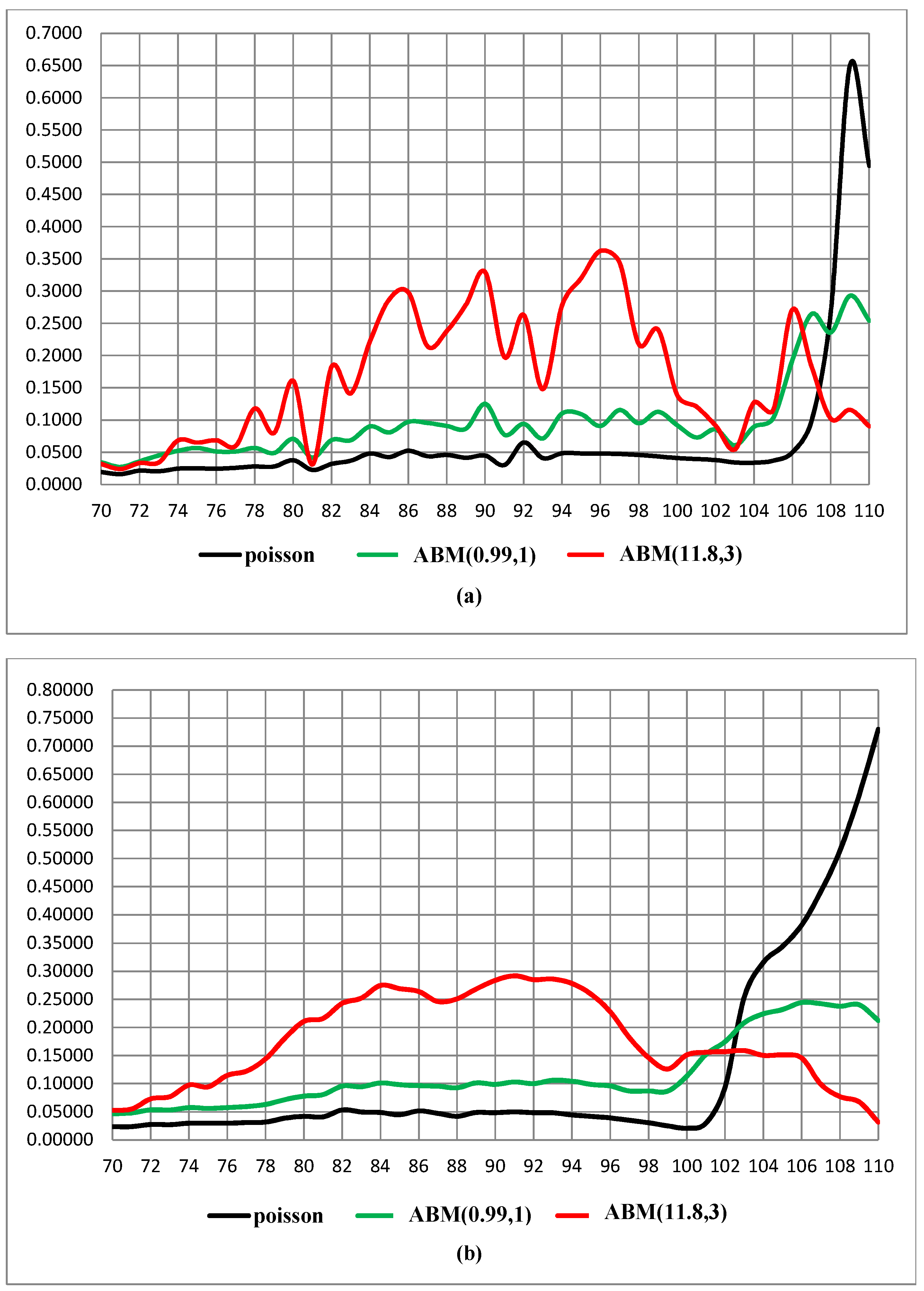
Figure 2.
RMSE for projecting mortality rate, USA, 2001–2007. (a) by age; (b) by cohort..

Figure 3.
RMSE for projecting mortality rate, Ukraine, 2001–2009. (a) by age; (b) by cohort..

Publisher’s Note: MDPI stays neutral with regard to jurisdictional claims in published maps and institutional affiliations. |
© 2022 by the authors. Licensee MDPI, Basel, Switzerland. This article is an open access article distributed under the terms and conditions of the Creative Commons Attribution (CC BY) license (https://creativecommons.org/licenses/by/4.0/).
Share and Cite
MDPI and ACS Style
Awad, Y.; Bar-Lev, S.K.; Makov, U. A New Class of Counting Distributions Embedded in the Lee–Carter Model for Mortality Projections: A Bayesian Approach. Risks 2022, 10, 111. https://doi.org/10.3390/risks10060111
AMA Style
Awad Y, Bar-Lev SK, Makov U. A New Class of Counting Distributions Embedded in the Lee–Carter Model for Mortality Projections: A Bayesian Approach. Risks. 2022; 10(6):111. https://doi.org/10.3390/risks10060111
Chicago/Turabian StyleAwad, Yaser, Shaul K. Bar-Lev, and Udi Makov. 2022. "A New Class of Counting Distributions Embedded in the Lee–Carter Model for Mortality Projections: A Bayesian Approach" Risks 10, no. 6: 111. https://doi.org/10.3390/risks10060111
Note that from the first issue of 2016, this journal uses article numbers instead of page numbers. See further details here.