Abstract
We construct a new age-specific mortality framework and implement an exemplar (DLGC) that provides an excellent fit to data from various countries and across long time periods while also providing accurate mortality forecasts by projecting parameters with ARIMA models. The model parameters have clear and reasonable interpretations that, after fitting, show stable time trends that react to major world mortality events. These trends are similar for countries with similar life-expectancies and capture mortality improvement, mortality structural change, and mortality compression over time. The parameter time plots can also be used to improve forecasting accuracy by suggesting training data periods and appropriate stochastic assumptions for parameters over time. We also give a quantitative analysis on what factors contribute to increased life expectancy and gender mortality differences during different age periods.
1. Introduction
A recent trend in mortality forecasting has been the development of models whose forecasts are robust to structural changes in mortality patterns. These include epidemiological changes, like the transition in major causes of death from infectious diseases to chronic diseases, and the decline in death rates due to chronic and degenerative diseases. For instance, Lin and Liu (2007) develop an insightful new type of model using a latent variable, “physiological age”, that aims to capture the aging mechanism. It has the potential to reveal trends in mortality and thereby allow the input of expert opinion about structural changes to mortality patterns. Other recent models incorporate automatic approaches to dealing with structural changes, such as by incorporating regime-switching behavior in the model itself Gylys and Šiaulys (2020); Milidonis et al. (2011). Most of these models do not directly incorporate the age-specific structure of mortality rates, which is known to follow a common shape across cultures and time periods Burger et al. (2012).
We introduce a framework for building parametric mortality models that captures the age-specific structure while using parameters with clear interpretations. We then demonstrate these aspects using a new parametric model as an exemplar of the framework: the Differential Logistic model with Growth rate and Controlling factor (DLGC). We show that the DLGC gives excellent and stable forecasts of future mortality, while at the same time revealing transient and structural changes in mortality patterns through the time plots of its parameters. Those patterns can then be used to fine-tune the forecasting method to give even better accuracy.
Most of the DLGC parameters reveal long-term trends, which, depending on the population being modeled, manifest either mortality improvement or mortality compression that arises naturally in tandem with mortality improvement at younger ages. The claimed interpretability of the parameters is justified in many examples where time plots of the fitted parameters reveal known historical mortality patterns. For instance, when fitting female data separately for the USA, Japan, France, and Switzerland, two of the parameters each revealed a sudden drop around the 1950s. Those drops are attributable to the vast and sudden decline in mortality during childbirth around that time in those countries. Mortality trends and structural changes in mortality patterns are context specific, and when fit, the DLGC reflects those differences. In some populations, we observe trends in specific parameters that represent mortality improvement, while in other populations, the trends in those same parameters are flattened or even reversed (always interpretable in those cases as “mortality compression” at higher ages). We also observed structural changes in one parameter in the mid-1990s in data only from Russia and Ukraine, but not from the other four (lower mortality) countries mentioned above.
DLGC is only one instance of the general framework introduced in Section 2 below. The advantages offered by the framework are:
- Familiarity and ease of implementation that comes with parametric models;
- Excellent fit; the exemplar of the framework, the DLGC, provides MSEs and AICs that are smaller than the Heligman–Pollard model Heligman and Pollard (1980);
- Good accuracy and stability in forecasting; projecting with the DLGC has comparable or better test MSEs in forecasting than the logit-binomial version of the Lee–Carter model, especially for 10-year-ahead forecasts. The forecasting accuracy is also more stable for DLGC than the logit-binomial Lee–Carter model, especially for those countries we examined with only intermediate overall life expectancy: Russia, Ukraine, and the USA.
- The structural changes in mortality revealed by DLGC provide insights that are useful for analyzing historical mortality and for improving forecasting. For example, parameter time plots not only give clues about historical structural changing times, but also help to select an appropriate historical data period to train the forecasting model, which is one of the main difficulties in mortality forecasting. Observed structural changes can also be used to suggest proper assumptions about parameter time series.
- Clear interpretation of each parameter: using the DLGC, trends are observed in almost all parameters; the trends provide evidence of mortality improvement or compression and can be used to quantify the proportion of improvement due to each parameter (see Section 3.5);
- Visibility of structural changes arising from the data, both transient (e.g., evident changes in mortality among French males during the World Wars) and persistent (e.g., observed sudden structural change in teenage female mortality around the 1950s); this allows objective, data-driven observation of structural changes without the need for the subjectivity that often backs expert opinion;
- Flexibility and interpretability of the framework: The framework is built starting with a heuristic modification of the logistic equation as a model for mortality with two functions and that are, respectively, interpreted as age-dependent mortality-decelerating factors (medical advances, broadly adopted healthy behaviors, etc.) and mortality-accelerating factors (aging, increasing pollution, etc.). The functions can be chosen to fit the context, and the DLGC shown below is the result of just one such choice. It shows stable and clear trends for parameters that match demographic characteristics, and it illustrates the model’s good interpretability.
We now place our new framework in the context of past literature. Mortality data are always organized by age, and mortality functions can additionally incorporate data groupings by period and/or cohort. From this perspective, models are grouped broadly into three categories depending on whether they use none, one, or both of the period/cohort groupings. Models incorporating all of age, period, and cohort as variables in the mortality function should, in principle, provide the best forecasts. However, the heavy data demands and the dependency between cohort, year, and age limit their uses. Continuous Mortality Investigation Bureau (2006) introduced a three-factor model that used p-spline regression and achieves a cohort forecast. Most research focuses on models grouping data as age-period or as age-cohort, and our approach considers only age-period.
Across a wide variety of modeling frameworks, it is often observed that mortality patterns are not purely deterministic, so forecasting models should include stochastic components. The most well-known example of this is the Lee and Carter (1992) age-time model, which uses many parameters and a single stochastic factor (see, for instance, Lee and Miller (2001), Booth et al. (2002), Renshaw and Haberman (2006) and He et al. (2021)). This model has several disadvantages (some shared by the many related models). When fitting, the model has an identifiability problem in which subjective constraints must be imposed to ensure that a unique choice of parameters will fit the data. It will also produce fitted mortality estimates that are not smooth functions of age.
In terms of forecasting, by including a single factor driving mortality improvement, Lee–Carter produces plausible forecast trends and allows a changing age pattern of mortality. However, its fixed-age pattern of change sometimes results in implausible age patterns over the long term, and it lacks smoothness across ages Booth and Tickle (2008). Callot et al. (2016) in 2016 also demonstrated that the dynamic model features of Lee–Carter are distorted by the deterministic trend component (i.e., a very strong negative time trend exhibited by age-specific log mortality) and suggest separating the deterministic and stochastic time series components to improve fit and forecasting performance. Furthermore, the Lee–Carter model assumes historical mortality patterns will hold for the future and no structural change will occur, which is not true for observed mortality patterns over the past century Lin and Liu (2007).
We adapt a separate established and common approach to mortality modeling and forecasting that begins by developing a parametric function describing the age-specific features of mortality that are observed regardless of the population being studied. For a given population and year, mortality almost always decreases sharply at young ages, increases quickly in teenage years or slightly later (often called an “accident hump”), and then increases through adulthood and into old age. The well-known Heligman–Pollard model Heligman and Pollard (1980) has three terms capturing the mortality in childhood, young adulthood (the accident hump), and senescence; it uses eight parameters across those terms. The five-parameter Siler model Siler (1979) also includes three independent terms presenting mortality during immaturity, adulthood, and old ages; it assumes a background mortality that is independent of age. Other examples of age-specific models include Rogers and Planck (1983), Carriere (1992), Hannerz (2001) and de Beer and Janssen (2016).
A function modeling mortality by age is by nature descriptive, but it can be converted to a stochastic forecasting model by fitting the model repeatedly to many years of data and then applying time series methods to the fitted parameters; see for example McNown and Rogers (1989) or Njenga and Sherris (2020), which both start with the Heligman–Pollard model for the age-specific mortality structure. These are multi-factor forecasting models: most or all parameters in the model are viewed as driving the stochastic mortality patterns. McNown and Rogers let each parameter be modeled by a separate ARIMA process. Njenga and Sherris take the more sophisticated approach of using vector error correction models (VECR), which account for cross-correlation or cointegration between these processes, as well as using a Bayesian VAR model for comparison as a way to assess parameter risk as it contributes to overall mortality uncertainty. Incorporating these multivariate forecasting methods significantly improved the forecast accuracy. The general methodology of fitting a parametric age-specific function and forecasting the parameters always leads to smooth forecasts across ages. It is usually easier to interpret the parameters and terms than with other approaches, such as the many-parameter Lee–Carter model and its extensions. Moreover, parameter time series often show clearer trends through time than those when using an extension of Lee–Carter.
We began with the observation that most of the parametric age-specific models cited above incorporate some parameters that do not have a clear connection to a variable observable or describable in terms of the mortality context. They also lack flexibility in the model itself: while certain features of mortality curves are universal, there are, of course, differences that are specific to the population and time period being considered. The framework introduced in Section 2 is broadly an age-specific model with three terms representing mortality in young childhood, in teenage years/early adulthood, and in adulthood and old age, as is now standard when modeling the entire mortality distribution (for instance, in the Heligman–Pollard model or the CODE model Bardoutsos et al. (2018); Heligman and Pollard (1980)). As mentioned above, we designed the model so that each parameter would have a clear interpretation in the context of mortality; we also kept the “accident hump”, as well as a background mortality. Following standard practice, we used simpler functional forms for infant and teenage mortality than for senescent mortality, but allowed flexibility in choosing the latter component.
The most interesting part of the framework is the component representing mortality in adulthood and old age. The Perks model Perks (1932) first proposed a logistic model for the force of mortality at high ages, and many well-known later studies have made similar assumptions Kannisto (1994). Modifying this idea and wanting to allow context-specific model adjustment, we began with the standard logistical differential equation and incorporated two functions of age, called and , to reflect the natural intuition that there are age-dependent factors that will accelerate mortality and others that will decelerate mortality. The two functions describing age-dependent mortality acceleration and deceleration can then be selected to have different functional forms depending on the context and the goals of the modeler. Altogether, a model produced within this framework has eight parameters plus however many are selected when specifying and .
We used the modified logistic equation as a heuristic, not claiming it as a law, but propose that the solution of the differential equation is a sensible way to model the part of the mortality distribution for old ages. Validation of this approach is provided by the points enumerated above: not just strong interpretation evidenced by general trends in parameters and functional forms for and showing decreasing and increasing trends that comport with intuition, but by the excellent fit to data, by excellent forecast accuracy, and from evident structural changes visible in the time plots of parameters. We expect that by examining more populations, over more time periods, with alternative choices for the functions and , a more nuanced understanding of mortality patterns will emerge.
Once the framework was developed, we created on specific age-specific mortality model, the DLGC, by selecting functional forms for and , bringing the total number of parameters to 14. Once we observed the good behavior of the parameter time plots and their ability to reveal structural changes, we set out to prove two points with forecasting: that the framework itself compared well with other models in terms of forecast accuracy and that the ability of the model to reveal structural change could be harnessed to improve the forecast accuracy. To forecast, we let each of the 14 parameters in the DLGC be a factor and forecasted each separately using an ARIMA model, following the approach of McNown and Rogers (1989). This approach served to prove the points just mentioned, but in future work, we plan to consider more carefully correlations and cointegrations between the parameter series by using VECR or BVAR multivariate forecasting models, as recently performed by Njenga and Sherris (2020).
To demonstrate the forecast accuracy afforded by the DLGC, we compared it with the logit-binomial version of the Lee–Carter model, performing validation both by comparing AICs with fits to historical data and by comparing five- and ten-year forecast accuracy, both across a variety of populations and then through a form of rolling-window cross-validation. The DLGC consistently outperformed the logit-binomial Lee–Carter model by each of these measures. (See Table 1, Table 2, Table 3, Table 4 and Table 5; in Table 3, Table 4 and Table 5, yellow indicates DLGC outperforming Lee-Carter and orange is the reverse. “HLE” and “ILE” refer to high-life-expectancy and intermediate-life-expectancy countries.).

Table 1.
AIC improvement between the Heligman–Pollard model and DLGC.
Table 2.
Comparing the fitting accuracy of DLGC and the Heligman–Pollard model for South Africa.
Table 3.
Comparing 5-year-ahead forecasts’ MSE[] of the logit-binomial Lee–Carter model and DLGC.
Table 4.
Comparing 10-year-ahead forecasts’ MSE[] of the logit-binomial Lee–Carter model and DLGC.
Table 5.
Five-year-ahead rolling-window cross-validation using USA male data.
More interesting, perhaps, is the second point: improving forecast accuracy by using the knowledge of structural changes revealed by parameter time plots. Some Lee–Carter modelers, such as Renshaw and Haberman (2003), have dealt with the problem of forecasting in the presence of changing mortality trends by including a second-order term in the singular-value decomposition underlying model, and while the forecast accuracy can be improved, the higher-order parameters were difficult to predict. Others have made a more fundamental shift by incorporating the potential for structural change into the model design, such as the regime-switching models employed by Milidonis et al. (2011) and Gylys and Šiaulys (2020). Originally used and well-developed in financial pricing, another advantage of regime-switching models is that they tend to be pricing friendly for mortality-based securities; many of them derive semi-closed or closed-form solutions for the concerned prices; see Gao (2015), Ignatieva et al. (2016) and Shen and Siu (2013). Like regime-switching mortality models, the methods underlying affine mortality models are borrowed from finance and are applicable to the pricing and risk management of mortality rates, e.g., Schrager (2006). Some recent mortality models combine affine and regime-changing characteristics, e.g., Blackburn and Sherris (2013).
We followed instead a simple approach to forecasting in the presence of structural changes taken by authors such as Tuljapulkar et al. (2000), Lee and Miller (2001) and Gylys and Šiaulys (2019): choosing to fit the model only to a shortened interval of years during which mortality patterns appear to be relatively stable. This allowed us to leverage the interpretability of the model parameters, which reveal changes in mortality patterns. As a case study, we identified two such structural changes and achieved considerably improved forecasting accuracy by choosing a significantly shorter time interval of training data that uses only data from after the changes revealed by the parameter plots from the fitted model. One could argue that this is only evidence that when forecasting with our method, older data quickly lose credibility. Therefore, we also tested this method over a time period with no observed structural changes and found that omitting older data instead decreased the forecast accuracy. In the future, we hope to run similar experiments with other models, i.e., we want to test whether we can improve other models’ forecasting performance by using training intervals suggested by DLGC.
This paper is organized as follows. Section 2 describes the construction of our framework, as well as the DLGC considered in this study. Section 3 shows the main results: goodness of fit and forecasting (Section 3.1); captured mortality improvement (Section 3.2); structural changes (Section 3.3 and Section 3.4); quantitative analysis on life expectancy (Section 3.5). Section 4 concludes.
2. Model Construction
2.1. Model Foundations
We begin by constructing an age-specific mortality model that predicts annual death probabilities; the target function we model is , the probability that a person age x dies before age .
We separate the probability into three components:
We interpreted as the contribution to mortality of factors arising during the youngest ages. In all contexts, this function starts from a high mortality rate near birth and decreases rapidly to 0 in a few years. We used the functional form for arising from the well-known Heligman–Pollard model Heligman and Pollard (1980): . This leads us to define as:
Sharrow et al. (2013) give a table describing the parameters in this model. The parameter A reflects the level of child mortality; it is approximately equal to , the probability of dying between age 1 and age 2. Since and are nearly zero, which can be derived from the definitions of and in Equations (3) and (6), respectively, A is also approximately equal to . The parameter B is the difference between age 0 and age 1 mortality probabilities, i.e., or ; C is the decline in mortality during childhood. All of A, B, and C are between 0 and 1. During fitting, we set the upper bound and lower bounds of A, B, and C to be , , , following the fitting results in Sharrow et al. (2013). Our testing confirms that those bounds do not lead to loss of generality.
We interpreted the term (3) as the contribution to mortality of factors arising during teenage years. We assumed that the factors influencing infant mortality have dissipated, while those factors leading to mortality in adulthood have not yet taken effect, so dominates and the other terms and in the model (1) are very near 0. During the teenage years, mortality increases, but is bounded, so as people move into adulthood, the mortality accumulated from factors is assumed to approach a limiting value, which then serves as background mortality in adulthood and old age. In this period, mortality data in almost all contexts show a relatively strong increasing pattern, especially at and near the “accident hump”. The model of Heligman and Pollard (1980) catches the sudden increasing pattern, but not a background mortality. The Siler model Siler (1979) includes a background mortality, but not the hump.
The logistic model has the desirable properties mentioned above, so we define as:
This arises in the usual way from the differential equation and initial condition:
The parameter is the limiting contribution to mortality from factors arising during the teenage years and the parameter is its growth rate. The age z represents the age at which this function grows fastest, so is interpreted as the age of the “accident hump”—from the functional form, at the age . When fitting, we bound , k, and z by assuming , , , where the upper bounds of and k are checked by experiments to be appropriate.
In the model (1), we interpreted the term as the contribution to mortality from factors arising during adulthood and old age. During those ages, we assumed that the contribution factors influencing infant mortality are negligible and background mortality coming out of the teenage years is stable at , so the increase in is dominated by the change in the term . We assumed that also has a limiting value. A logistic function would again have the requisite properties and has been commonly used in earlier work as the model for the component associated with old age.
We adopted instead a framework for creating a generalized form of logistic function to model . It still assumes a limiting mortality in the oldest ages, and besides effects counted in this value, the framework incorporates two types of age-dependent factors affecting mortality in adulthood: those with an accelerative effect on mortality and beneficial factors with a decelerative effect. For example, we would regard beneficial factors to include medical improvements, improved access to food and resources, avoiding risky activities, taking beneficial supplements, preventative medical care, and similar human actions, which would decelerate mortality, but often with contributions that depend on age.
We represent the cumulative effect of beneficial, mortality-controlling factors by and the cumulative effects of factors accelerating mortality by . Our generalized logistic model begins with the underlying logistic differential equation, modified to include as an accelerative factor and as a decelerative factor:
The parameters involved all have simple interpretations, as follows:
- : the maximum value of the contribution to one-year mortality from factors arising during adulthood and old ages. At extreme old age x, we have , which is the overall asymptotic mortality.
- : the age at which the function is half of its maximum. The main process causing to increase is happening fastest near .
- An increasing function of age with range : this represents the effect of natural factors cumulatively accelerating the mortality probability during adulthood and old ages. Such factors include biological aging processes and lifestyle patterns with a harmful effect. This adds nuance not found in the teenage term , which adopts the same model, but with a constant growth factor k. We view this as sensible because the increasing process during teenage years happens in a much shorter time period than that during old ages. The aging effect on mortality is obviously stronger at older ages. Therefore, we assumeed is increasing over age during this period. Without any beneficial factors decelerating mortality, would satisfy the special case of (5) with .
- A function of age with range : this represents the effects of beneficial factors decelerating mortality probabilities. We require that for any age x, in order to keep positive always. Furthermore, we require , since if , the function no longer represents a decelerative effect in the model (5). During ages with , beneficial factors and human actions controlling mortality are contributing to slow the mortality growing. During the ages with , these beneficial factors and actions have no extra beneficial effect on mortality compared to the asymptotic effect counted in g and the processes contributing to .
The parameter g is the major age-independent contribution to mortality at the oldest ages, and and can be viewed as age-dependent adjustments to g that can be chosen based on context. For g to have this interpretation, the differential Equation (5) imposes the additional constraint that is approximately 1 in the oldest ages.
After solving the differential equation system (5), we derive the function form of :
where denotes the average value of on , i.e., .
When fitting, we assumed that values are in and that , following the CODE model Bardoutsos et al. (2018), which assumes that .
2.2. The General Framework for Modeling Mortality
To summarize the full framework: is the one-year mortality probability for a life aged x. Based on (1), (2), (3), and (6), we can have the general model formula for .
This model includes eight constant parameters and two functions and chosen for one’s convenience and needs. This framework is not only flexible: it can give highly accurate fits as well, as will be shown in later sections.
Here is a table recording a brief description of all parameters and functions involved in the general form of the model.
2.3. DLGC: Death Probability Model with Chosen and
We now specialize to a model with particular choices for parametric forms of and that we call the DLGC, for “Differential Logistic model with Growth rate and Controlling factor”. We will fit the DLGC to mortality data in later sections.
As is naturally expected to be an increasing function, the DLGC applies an increasing logistic function for :
With this definition, we introduced four new parameters. At the younger ages of adulthood, we are assuming that the mortality acceleration factor keeps at or near the lower level . As the natural accelerating factors such as biological aging processes show relatively more and more obvious effects on mortality in older ages, we assumed that the acceleration factors increase toward a higher level at older ages. The fastest period of growth in happens at and near the age , and near this age, the accelerating factors would show the largest effect over a short time. The rate of increase of around this age is controlled by . With a larger value of , the main increase in occurs more drastically and over a shorter time. At ages well past , the function approaches a value near the higher level and levels off, so we are assuming the effects of these accelerative factors are not unlimited
For the function describing beneficial, decelerative factors, we chose the function:
introducing two more parameters to the model and satisfying the stipulations in Table 6 as well. In , we partitioned the ages of adulthood into three parts: before age 65, between age 65 and 85, and after age 85. The parameter represents the approximate average level of the decelerative factor for the lowest age group, while represents the approximate average level in the middle age group. We assumed that is approximately 1 at very old ages, i.e., that beneficial factors, especially those arising from human activity, have a limited effect at the oldest ages.
Table 6.
Parameters and functions assigned in the general model of .
We assumed that the changes between levels follow the logistic form. The location of the changes between levels were fixed at 65 and 85, rather than included as parameters, because we already obtained good fits and see no obvious benefit from including two additional parameters.
After choosing above and , we derived the model for as
where satisfies (9), satisfies (8), and (the average value of on ) satisfies the following:
The above is the precise description of the DLGC, which includes 14 constant parameters to model the death probability . Below is a table describing all the parameters.
When fitting, we bound , , , , , and by assuming , , , , , . The bounds for , , and were suggested by the CODE model Bardoutsos et al. (2018), and the upper bounds of , were checked by experiments to be appropriate.
2.4. MSE Minimization
We used a weighted MSE to fit the model and to measure goodness of fit. Bardoutsos et al. (2018) state that the mean-squared error (MSE) of gives a relatively large amount of weight to errors at young ages, the MSE of gives more weight to errors at old ages, and the MSE of , i.e., death rate at age x, gives more weight to errors around the modal age. As a result, we minimized the weighted MSE, denoted as , satisfying
to estimate our parameters, using the reciprocals of the data variances as weights. Here, are the measured mortality probabilities taken from period life tables in the Human Mortality Database (HMD) Wilmoth et al. (2007). The value is the death rate at age x derived from our fitted using the same life table calculations used in the HMD. We also calculated the from the weighted MSE, so that our model was fit by maximizing . We used values of near 100% as evidence of a good fit to the data.
2.5. Modal Age M Fitting
Once we have fit for non-negative integer x, we estimated the modal age of death as well, denoted as M. We assumed the force of mortality at age x, , is piecewise constant, satisfying
with constants . Since , we have for Therefore, we are able to fit the modal age M by
2.6. Mortality Forecasting with DLGC
We can extend the DLGC to forecast future mortality. For each calendar year, t, assume that the death rate, , follows the DLGC Equation (10), and denote the fourteen embedded parameters as , , , , , , , , , , , , , . Since the parameter values change for each year, they naturally form time series: , , , , , , , , , , , , , . To use those series for forecasting, assume:
- , , , , have values whose logs form random walks with drift, e.g., satisfies , where is the drift term and are normally distributed i.i.d. error terms;
- , , , , , , , have values that form random walks with drift, e.g., satisfies , where is the drift and are normally distributed i.i.d. error terms.
This simple approach using univariate ARIMA models for each parameter, pioneered by McNown and Rogers (1989), provides accurate forecasts in our context (see Section 3.1.2). Moreover, in Section 3.4, we significantly improve forecast accuracy by choosing a window of training data suggested by observed structural changes.
To project future values of , apply Equation (10) using the projected values of the time series. The MSE of the forecast test results and the stable tendency of the majority of the parameters (analyzed in Section 3.2) support the assumptions used in the mortality forecasting.
3. Main Results of DLGC
In this section, we analyze by age and year mortality data drawn from the Human Mortality Database (Human Mortality Database n.d.). We performed all data analysis using the statistical software R (R Core Team 2021). We used data for six countries, which we split into a group of four and a group of two based on average life expectancy at birth. For the ease of exposition, we give names to these groups:
- HLE countries
- France, Japan, Switzerland, and the USA have relatively high life expectancy at birth;
- ILE countries
- Russia and Ukraine have intermediate life expectancy at birth.
We focused primarily on the years 1959 to 2013, when the data for all six countries are available, although occasionally, we examined earlier years.
For each year of available data, we fit the DLGC to observed values of from the HMD using all ages x from 0 to 100. We truncated at age 100 because the data on supercentenarians in the HMD has been smoothed. In yearly data fitting, we used the R package DEoptim Mullen et al. (2011), which performs global optimization by differential evolution.
After fitting yearly data for all years with data available for all six countries, fitting each gender separately, we forecast mortality for each population using the R package forecast Hyndman and Khandakar (2008). Viewing each parameter as a time series, we modeled either the parameter or its log as a random walk with drift, as this seemed appropriate. We used 26 years of fit parameters and forecast each parameter out 5 years or 10 years, from which we obtained forecast mortality curves. Using data for these same years from the HMD as a validation set, we compared the test error of our forecast with that from a logit-binomial version of the Lee–Carter model in the R package StMoMo Villegas et al. (2018) by using the function lc.
In Section 3.1, we show that DLGC gives an excellent fit for every dataset—for each country and gender, the mean across the years is always bigger than 99%. It also provides a good forecast accuracy for each population, especially in ILE countries. We examine the variation of the fitted parameters through time in Section 3.2 and Section 3.3, interpreting trends and some mortality structural changes, including the influence of major wars. Section 3.4 shows the structural changes observed help improve forecasting accuracy. In Section 3.5, we give a quantitative analysis of parameter influence on life expectancy improvement and the gender gap.
3.1. Goodness of Fit for DLGC
3.1.1. Fits across Age
For each of the four HLE countries France, Japan, Switzerland, and the USA and each of the two ILE countries, Russia and Ukraine, we fit the DLGC to female, male, and total (both female and male) datasets in all data available years.1 The summary of the fit, measured by described in Section 2.4, is recorded in Table 7:
Table 7.
of the DLGC fitting results.
- Overall, the DLGC gives an excellent fit. For all datasets, we averaged the values across all fitted years for a given country and gender. All means were above 99%. The lowest was 99.55%, occurring for Russian males, and the highest mean was 99.94% for Japanese females.We also fit the Heligman–Pollard model Heligman and Pollard (1980) to the six countries’ data for all available years by maximizing the , to compare the goodness of fit with the DLGC model. (The year period for each country is the same as Table 7.) Table 8 summarizes the fit.
Table 8. of the Heligman–Pollard model fitting results.The means of for the fitted Heligman–Pollard model were between 93.18% and 96.68% for the six countries, while for DLGC, they were all above 99%. Overall, the DLGC shows much better accuracy than the Heligman–Pollard model does across countries and gender. Several particularly poor fits of the Heligman–Pollard have 71.74% for French male total population in 1915, 76.83% for Russian males in 1994, and 76.43% for Ukrainian males in 2005, while DLGC’s results are all above 91.90%. DLGC fits better than the Heligman–Pollard model on data from both recent years and from those over a century ago.Since our model has more parameters than some others, we also compared it against other models based on the AIC, defined aswhere k is the number of parameters in the model under consideration and n is the number of observations.The DLGC also performs better than the Heligman–Pollard model with respect to the AIC. This is observed universally among the six countries, for both female and male populations, both recent years and older years. For example, as one HLE country, the fitting results of Switzerland female have an AIC −1240.87 (DLGC) compared with −741.88 (Heligman–Pollard) in 2018, −1134.83 (DLGC) compared with −702.34 (Heligman–Pollard) in 1886; in 2013, as one ILE country, the fitting results of Russia have an AIC −1228.57 (DLGC) compared with −962.35 (Heligman–Pollard) for female and −1139.05 (DLGC) compared with −984.77 (Heligman Pollard) for male. We recorded the AIC improvement, i.e., , in each year’s data fitting for both genders in all six countries. Table 1 summarizes the ’s mean among years with available data shown in Table 7. One can notice that, by including 14 parameters, 6 more parameters than the Heligman–Pollard model with 8 parameters, the DLGC obtains great improvement in its fitting accuracy and is not overfitting.
- The DLGC sometimes gives a noticeably worse fit during a year that a country was at war. This is especially evident for French males during the World Wars. The eight years for which the for French total male population was less than 98.5% were 1914–1918 (exactly the span of World War I) and 1940, 1943, and 1944 (during World War II). By contrast, Switzerland maintained neutrality during the World Wars, and the fit to Swiss male data is not noticeably worse during the war years. Overall, the French civilian male population is fit better than the French total male population in the mean, SD, and range. Excluding the eight war years mentioned above, the fitting results for French total male population in all the remaining years have a mean of 99.75% and SD 0.00185, with a range of 98.94% to 99.94%. These are in line with the French civilian male data, especially if we remove 1919, the single year for which the model produced under 98% (at 96.17%) when fitting French civilian males. Excluding 1919, the French civilian males in all other available years have a mean of 99.75% and SD of 0.00198, with a range of 98.84% to 99.95%, almost identical to the values for French total males with the war years excluded. It is possible that the poorer fit for French civilian males in 1919 compared with other years is a continuation of the anomalous fit seen for total male population during war years: there was likely a number of soldiers who transitioned to civilian life immediately after the war and then died some months later in 1919, from wounds or other factors incurred during service.
- Excluding war years, the DLGC is observed to fit data from HLE countries better than ILE countries. Among the six countries, DLGC gives the best fit for for Japan and the USA, where the is at least 99.57% for all female, male, and total datasets over all available years of data. For Switzerland, over 144 years, the minimum is 99.26%. As mentioned above, for French data over the last 200 years, excluding the war years mentioned above, the minimum is 98.94%. Compared with these high-life-expectancy-at-birth countries, Russia and Ukraine show lower means, higher SDs, and lower minimum (still higher than 97.6%).
- For the four HLE countries, France, Japan, Switzerland, and the USA, the DLGC tends to fit better for female datasets than male datasets. For these countries, the mean for females is higher than that for males during the same time period, and the minimal appears with a male dataset, such as 91.90% for French total male population in 1915 and 96.42% for French civilian male population in 1919. The minimum for female data is at least 98% for all HLE countries and all years. For the two ILE countries, Russia and Ukraine, there is no clear distinction between for females and males.
- The fit is better in more recent years for all countries with data extending into the Nineteenth Century. For French civilian males over the period 1816–1917, the mean is 99.64%, and for females, the mean is 99.77%. For the period 1918–2018, the mean for French civilian males is 99.82%, and for females, the mean is 99.92%.
We now briefly consider how DLGC models mortality from South Africa, a low life expectancy country. Because of the limited availability of online mortality data for South Africa, we only tested a more recent period ( by age and year life tables in 2006–2008) and an older period ( by age and year life tables in 1925–1927) for both genders, using data drawn from the Human Life Table Database Human Life Table Database (n.d.). Table 2 summarizes the DLGC fitting accuracy by and the AIC and compares it to the Heligman–Pollard model, showing that the DLGC fits South Africa well.
3.1.2. Forecasting over Years
To examine the forecasting accuracy of DLGC, we compared it to the logit-binomial version of the Lee–Carter model (in the R package StMoMo Villegas et al. (2018)). For every population, we used the same training data to fit the two models and then compared their (mean-squared error of death rate) for forecasts of the following 5-year or 10-year period using available mortality data.
For the four HLE countries, we used data from years 1990 to 2015 and ages 0 to 100 to train the two models and forecast the following 5-year period (i.e., 2016 to 2020) as a shorter-term forecast. For longer-term forecasts, we trained the models on data for years 1985 to 2010 and ages 0 to 100 and forecast the following 10-year period (i.e., 2011 to 2020).
Since data for the two ILE countries are only available until 2014, we trained the models on data from years 1984 to 2009 and ages 0 to 100 and forecast from 2010 to 2014 as the shorter-term forecasting. For the longer-term forecast, we trained the models on data from years 1979 to 2004 and ages 0 to 100 and forecast from 2005 to 2014.
Table 3 and Table 4 summarize the test forecasting MSE[] in six countries for both genders for the recent 5-year-ahead and 10-year-ahead forecasts, respectively. Blocks where DLGC has a better test MSE[] than the logit-binomial Lee–Carter model are marked as yellow, while blocks where DLGC performs worse are marked as orange. The grey blocks indicate that data are unavailable for those years:
- In summary, DLGC has better forecasting accuracy than the logit-binomial Lee–Carter model. For the 186 years of death rate data, DLGC performs better on 81.18% of them (151 out of 186). For all test samples, DLGC’s MSE[] is below , while 9.14% (17 out of 186) of the logit-binomial Lee–Carter’s MSE[] are bigger than (and its largest MSE[] is ).
- Table 3 and Table 4 show that DLGC’s superiority to the logit-binomial Lee–Carter model is more pronounced for the longer forecasting period. In 5-year-ahead forecasts, DLGC performs better on 67.24% of test samples (39 out of 58), but in 10-year-ahead forecasts, the proportion rises to 87.50% (112 out of 128). Results for Switzerland and Japan repeat that pattern. For Switzerland, DLGC performs worse in the 5-year-ahead forecasts (2 yellow vs. 8 orange), but forecasts better on almost all 10-year-ahead tests (19 yellow vs. 1 orange). For Japan, DLGC and the logit-binomial Lee–Carter tie (5 yellow vs. 5 orange) for the 5-year-ahead forecasts, but DLGC is much better in the 10-year-ahead tests (19 yellow vs. 1 orange).
- For HLE countries, both models provide very accurate forecasts, but for ILE countries and the USA (which has the lowest life expectancy among the four HLE countries), DLGC’s forecasts are more stable, i.e., the total growth of over time is much smaller for DLGC than for the logit-binomial Lee–Carter, except for Ukraine females, where the comparison is distorted because the latter model has a much worse forecast in the first year.
- DLGC’s superiority to the logit-binomial Lee–Carter model is more pronounced for ILE countries. In both 5-year-ahead and 10-year-ahead forecasts, DLGC forecasts are almost always better (and stabler) for the two ILE countries and the USA. Comparing HLE and ILE countries, there are 21 yellow blocks out of 40 (52.5%) in 5-year-ahead forecasts and 75 yellow blocks out of 90 (83.33%) in 10-year-ahead forecasts for HLE countries, while for all test samples in ILE countries, there are 18 yellow blocks out of 18 (100%) in 5-year-ahead forecasts and 37 yellow blocks out of 38 (97.27%) in 10-year-ahead forecasts.
- DLGC forecasts better than the logit-binomial Lee–Carter model for both males and females, but the superiority appears similar for each gender. In 5-year-ahead forecasts with 29 test samples in each gender, 21 are yellow for female and 17 are yellow for male; in 10-year-ahead forecasts with 64 test samples in each gender, 57 are yellow for female and 55 are yellow for male.
Figure 1 plots the Russia male 2014 death rate forecasting of DLGC and the logit-binomial Lee–Carter model by fitting data from 1979 to 2004.
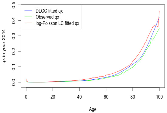
Figure 1.
RUS male 2014 death rate forecasting of DLGC and the logit-binomial Lee–Carter model.
Figure 2 plots the USA male 2019 death rate forecasting log value of DLGC and the logit-binomial Lee–Carter model by fitting data from 1985 to 2010.
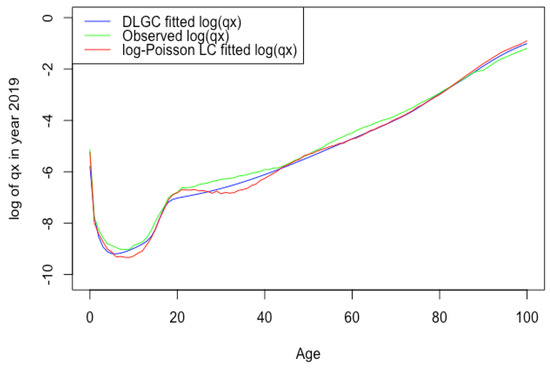
Figure 2.
USA male 2019 death rate forecasting log value of DLGC and the logit-binomial Lee-Carter model.
The above data were all from one time period. To further validate the DLGC, we performed a form of rolling-window cross-validation as in, for instance, SriDaran et al. (2022). The MSEs of 5-year-ahead forecasts of the two models were compared after training the models on data for USA males with time intervals starting with 1975–2000 and rolling forward one year at a time. The results are presented in Table 5 and show that DLGC outperformed the logit binomial Lee–Carter model. (Blocks are marked yellow if DLGC outperforms and marked orange if the logit-binomial Lee–Carter model outperforms.)
3.2. Variation of Parameters through Time
This section examines the trends of the fitted parameters through time, focusing specifically on parameters that show a relationship with mortality improvement, as well as differences in parameter levels and trends between countries and between genders. We primarily focus on the years 1959 to 2013, when the data for all six countries are available.2
The greatest mortality improvement is observed in HLE countries, as may be expected. This pattern is manifest in parameters from all three age groups—children, teenagers/young adults, and older adults. Indeed, the countries within the HLE and ILE groups show surprising consistency across a number of measures, such as the the change in parameter level or variance over time. By contrast, for some parameters, there are obvious differences between the two groups.
Mortality improvement at younger ages is evident simply in a decrease in the value of , but mortality improvement in older ages is generally observed to lead to compression and increased mortality at the oldest ages, because delaying the age at death increases the number of people at the highest ages and the proportion of people dying at those ages. We must therefore be more careful in describing the relationship between mortality improvement and the model parameters associated with old ages.
Summary of observations: We observed mortality improvement associated with lower infant mortality through downward trends in the parameters A and C. Mortality improvement among teenagers was observed just in one parameter, a decrease in the limiting teenage mortality , and only in HLE countries. Mortality improvement at old ages was observed in HLE countries through a modest decline in the limiting mortality g (except remaining flat in the USA) and an increase in the age at which fastest growth occurs in the model. Among the parameters of the associated functions and , which represent age-dependent mortality acceleration and mortality deceleration factors, respectively, we observed mortality improvement in all countries evident in a delay in the age of fastest growth of the function , as well as in increasing trends in the levels and of the function at younger old ages. Finally, we observed mortality improvement through an increase in the modal age at death M computed from our fitted model in all countries.
Compression was evident in ILE countries through a combination of an increase in the age of fastest increase in the component of mortality for the oldest ages occurring together with an increase in the limiting mortality g at the oldest ages. Compression was observed in all countries through an increasing trend in the age at which the mortality acceleration factor increases fastest, combined with an increasing trend in , the approximate level of the morality acceleration factor above the age .
3.2.1. Mortality Improvement in the Earliest Ages
The three parameters in the DLGC related to childhood mortality are A, B, and C appearing in the function (see Table 9). For fixed x, the value decreases when any of A, B, or C decreases, so a decrease in these parameters is evidence of infant mortality improvement.
Table 9.
Parameters in DLGC.
Parameter A shows a similar time variation whether comparing different countries or genders. For all six countries, both HLE and ILE, from 1959 to 2013, the parameter A decreases over time, leading to a decrease in for all ages x. Thus, A contributes to infant mortality improvement in all cases. Moreover, decreases approximately linearly, implying that A has a nearly stable decay rate over this period.
The parameter A exhibits well the consistency within country groups and contrast between groups, as the time plots of were very similar for each country within each group. Figure 3 shows plots of from 1959–2013 when female data were fit to DLGC for each country and year, i.e., female infant mortality . The left plot is for the four HLE countries; the right is the ILE countries; we see the approximately linear decrease from similar levels in both plots in 1959 to much lower levels in the HLE plot by 2013. While all countries have shown improvement in infant mortality over this time period, the improvement has been more dramatic in HLE countries during this period. Thus, the parameter A was seemingly not contributing much to a difference in mortality between HLE and ILE countries in 1959, but has since been responsible for some of the greater mortality improvement in HLE countries.
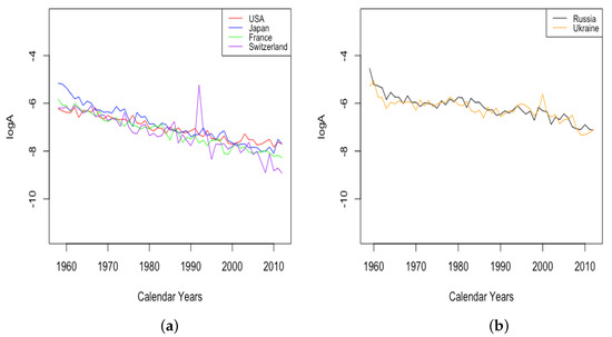
Figure 3.
(a) The log of infant mortality A for females from 1959 to 2013 across HLE countries. (b) The log of infant mortality A for females from 1959 to 2013 across ILE countries.
Comparing the plot of for males and females from a single country shows either no substantial difference or else a slightly lower curve for females than males. It is known that infant mortality is a little higher for males than females in most parts of the world, with several reasons being put forward Pongou (2013), so the curves produced by the DLGC are in line with the expectations.
While Figure 3 shows generally linear trends in for all six countries, examining all of the data from countries with older available data, France and Switzerland, shows that the trend has changed over time. Figure 4 shows the trend of for 203 years of fitted data for France and 142 years of fitted data from Switzerland. For both countries, infant mortality shows a relatively slow decline until the early 1900s, then a quicker decline, and France also shows slowing again in recent years, which is hard to see in the limited version in Figure 3.
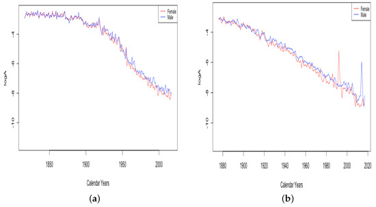
Figure 4.
(a) The log of infant mortality A in France, male vs. female. (b) The log of infant mortality A in Switzerland, male vs. female.
The parameter B shows no consistent trend, staying relatively flat for each country over time. There are differences between countries, however. Among the HLE countries, the largest contrast is between Japan and the USA. Figure 5 depicts the value of B for these countries over all years of available data. The value B is consistently higher for Japan than for the USA. Japan is the only one of the six countries exhibiting anything other than essentially flat behavior. It seems there was a sharp decline in the part of infant mortality attributed to B before 1960, and it is notable that in 1959, Japan had the lowest life expectancy at birth of 67.44 among all six countries, while in 2013, Japan had the highest life expectancy at birth of 83.47. It is not clear why B may have increased again in Japan since that time.
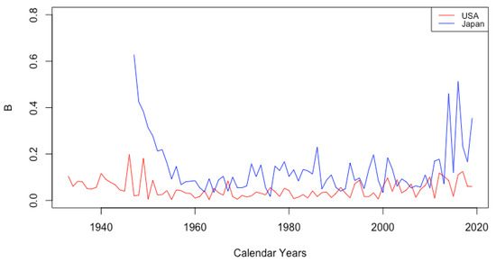
Figure 5.
Comparison of B between Japan and the USA.
The value for the ILE countries was generally higher than that for HLE countries. Interpreting B as a drop in between ages 0 and 1, this could be just a reflection of a higher probability for the ILE countries.
As shown in Figure 6, parameter C experienced a small decline between 1959 and 2013 for all countries except the USA, for which it remained essentially flat. The decline in C results from the infant mortality decreasing. Once again, C is somewhat larger for ILE countries than for HLE countries, suggesting that childhood mortality decreases faster in ILE countries than HLE countries, but that may be because there is a birth mortality gap between these two groups of countries. In Figure 6c, in France civilian population, C stays at a higher level before 1950s, decreases rapidly during 1950–60s, and then, levels off at a lower level after that.
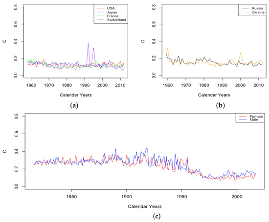
Figure 6.
(a) Decline in mortality during childhood, i.e., C, across HLE countries. (b) Decline in mortality during childhood, i.e., C, across ILE countries. (c) Decline in mortality during childhood, i.e., C, for France civilian population, male vs. female.
3.2.2. Mortality Improvement in Teenagers
The three parameters in the DLGC related to teenage/twenty-something mortality are k, z, and appearing in the function (see Table 9). For fixed x, the value decreases when or k decreases and when z increases, so these changes would indicate mortality improvement. This is intuitive for and z, since is the upper bound and limiting value for mortality caused by factors during teenage years, while an increase in z is a shift of the “accident hump” to a later age.
The parameter k was observed to be stable for all six countries, with occasional spikes above the stable level, seemingly random. More interesting behavior is exhibited by the other parameters.
We expect z to fall in a relatively small range of ages since it represents the age of the “accident hump”. It should not be able to trend up or down indefinitely; yet, there is also no particular limiting value that should be expected through biological mechanisms. It is not surprising, then, that over long time periods, the fitted z value is observed to wander up and down within the range of ages when it is typically observed.
Since 1960, the fitted z for HLE countries has mostly between 13.5 and 18, while the value for ILE countries has remained higher between about 16 and 21 until 2000 and has increased from 20 up to the low 20s for Russia and the mid-20s for Ukraine since the year 2000. In all countries, the fitted z for males is only rarely observed to be lower than females. The gap is generally observed to be smaller in HLE countries and to be negligible some of the time. In the ILE countries over all available data since 1959, the z for male data has almost always been 1–3 years higher than the z for female data, except in the growth period since 2000, when both datasets experienced comparable levels.
Figure 7 gives an example plot of for Switzerland for the long period 1876–2018 and for Ukraine for 1959–2013. All six countries were at fairly comparable levels in 1959. Comparing just the period from 1959–2013, the HLE countries all experienced a decline in , with each country except the USA showing continual improvement. For the USA, has remained flat since around 1970. By contrast, the ILE countries have experienced a moderate increase, as seen for Ukraine in the panel on the right. Since 1959, it seems the limiting mortality has been a factor in teenage mortality improvement for HLE countries, but not in ILE countries. For Russia and Ukraine, the combined effect of the recent trends in z and is that the average accident hump is occurring at a later age, and after the hump, the mortality climbs to a higher background level.
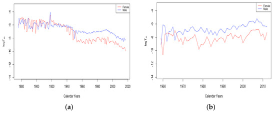
Figure 7.
(a) The log of the limiting teenage mortality for Switzerland, male vs. female. (b) The log of the limiting teenage mortality for Ukraine, male vs. female.
A striking feature of the above plot of is the sudden transition of the female mortality in Switzerland around 1950. While both curves generally trend down and are relatively close together until that year, the female curve exhibits essentially a discontinuity with a sudden improvement in the value . This seems to be a permanent change, and females have continued to have a drastically better value of than males ever since. All four of the HLE countries show this transition sometime during the 1950s. We see no transition in the plot of Ukrainian data on the right, but since the curves are separate with females below males for essentially the whole period, we assume that if data existed extending back through the 1950s, we may very well have seen this transition in the ILE countries as well. We will discuss the transition in more detail in Section 3.3.
The final feature to note here is the small spike in in Switzerland in the year 1918, a spike that is more evident in the plot of itself. French total population exhibits three periods of spikes in : the years 1870–1871, the years 1914–1918, and the years 1940–1943. We will return to consider these spikes in more detail in Section 3.3.
3.2.3. Mortality Improvement in Adulthood and Old Age
There are eight parameters in the version of the DLGC we implemented (recall that other versions can be produced by using different functions and )— and g are in the function regardless of how the framework is implemented, while , , , , , and were parameters in the particular functions and we chose when implementing the model (see Table 9).
Mortality improvement is generally observed to lead to compression and increased mortality at the oldest ages, so the oldest people will experience higher mortality even as the younger population is considered to be undergoing mortality improvement. We must then be more careful in specifying the relationship between these parameters and mortality improvement than we were in the previous sections. For instance, the parameter g is the limiting mortality for the component related to factors arising during adulthood and old age, and the parameter is the age at which has risen to half of that limiting value. An increase in g could be viewed as mortality getting worse, but if simultaneously accompanied by a large increase in , it could instead just be an indication of an increase in the age at which mortality increases fastest followed by a higher limiting value in the region of mortality compression. Regardless, we view either an increase in or a decrease in g as direct evidence of mortality improvement.
The model (5) incorporates as a factor causing mortality deceleration and as causing mortality acceleration. Thus, increases in the values of and , the approximate heights of below age 65 and between ages 65 and 85, should be viewed as mortality improvement. Similarly, we view decreases in the values of , , and as mortality improvement, as well as an increase in the age . We note that a second instance of mortality compression can be manifest in an increase in occurring simultaneously with an increase in , analogous to the situation with g and described above. We could then still view this as a form of morality improvement.
Finally, while the modal age at death is not a parameter in the model, we computed it from the fitted model as described in Section 2.5. We naturally view an increase in the modal age as mortality improvement.
Summary: Overall, we find that in all six countries, mortality improvement is substantially impacted by parameters associated with mortality in adulthood and old age. For these countries, almost all of the above-mentioned parameters in have trends that either show mortality improvement or else give evidence for compression.
For the four high-life-expectancy-at-birth countries, a decline in maximum mortality g (except in the USA, where it remained flat), an increase in the age at which the main increasing process in is occurring, and increases in the overall level of the mortality deceleration function all indicate mortality improvement coming from factors arising during adulthood and old ages. For the ILE countries, we observed increasing levels of g combined with a delay in the age , which, together, are evidence of compression, as well as increases in the overall level of the mortality deceleration function . For all countries, we observed evidence for compression in the form of an increase in the level of the mortality acceleration function at the oldest ages, as well as a delay in the age at which the increase to this level is occurring.
Limiting mortality and the age of fastest growth
Figure 8 shows how g, the limiting mortality caused by factors arising in adulthood and old age, changes over time for the six countries over the period when all countries have data. The HLE countries each experienced a modest decline, except the USA, for which g has remained essentially flat. The other countries caught up to the USA, reaching levels at the end of the time interval comparable with what the USA had experienced for decades. By contrast, the trend in g has been remarkably consistent in the ILE countries, with both curves staying close together through periods of slow growth, then faster growth, and then slow growth again—drastically different behavior than the gradual decline among the HLE countries.
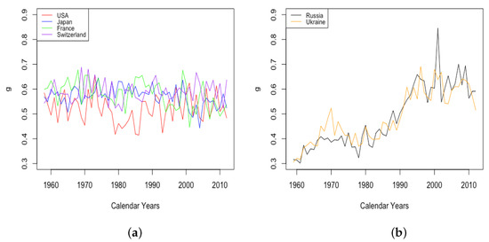
Figure 8.
(a) Limiting old age mortality g across HLE countries. (b) Limiting old age mortality g across ILE countries.
By comparison, the age at which the sharpest increase in occurs, also the point at which half of the limiting value is obtained, is observed to increase steadily among all six countries, although at different levels and rates (see Figure 9). Japan experienced the most drastic growth, from the lowest value among HLE countries of 92 in 1959 up to the highest observed value of 98 in 2013. By contrast, the value M1 for the USA experienced an increase of just 1 year or so through the same period. The value of for ILE countries was lower than that of HLE countries over this period, but showed an increase almost as large as that of Japan, so that by 2013, the value was comparable to the lowest values among the HLE countries.
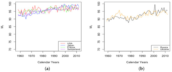
Figure 9.
(a) Age of fastest increase in senescent mortality across HLE countries. (b) Age of fastest increase in senescent mortality across ILE countries.
It is clear then that both parameters g and have contributed to mortality improvement for the HLE countries, with a lower limiting value approached at a later age. The situation with the ILE countries is more complicated—as mentioned above, the observed increase in g is not necessarily mortality getting worse because it was accompanied by a simultaneous delay in the age at which the growth toward that limiting value occurred, which we view as indicative of compression.
Figure 10 also shows how the parameter g changed over the last two centuries for French females. The limiting old age mortality g was increasing from 1816 to the early 20th Century and then started to decline after that. By contrast, the parameter increased from an average level around the high 80s in the early 19th Century up to the high 90s by the 21st Century. Thus, it appears that mortality improvement occurred over this entire period, but in the form of compression until the 20th Century and then more direct improvement since then.
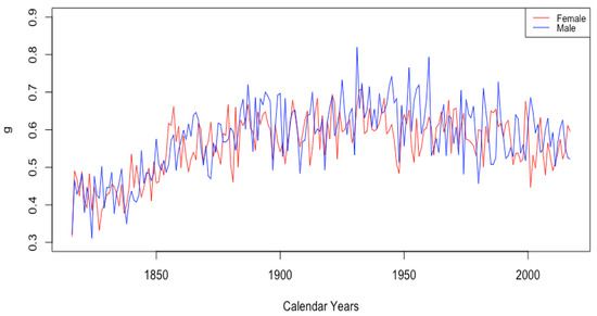
Figure 10.
Limiting old age mortality g for France civilian females during 1816 to 2018.
Mortality acceleration factor with parameters
The mortality caused only by factors during adulthood and old age, , involves the mortality acceleration function . For the DLGC, we chose the particular form of in Equation (8), a function that increases from a level to level , with the age of fastest growth and a growth rate.
For HLE countries, the plot of in Figure 11 shows large variance until around the 1950s, followed by a gradual decrease in the variance. The upper limit of is around 90 for the entire plot, but the lowest observed values gradually increase over time until values for all four countries stabilize between about 75 and 90 around 2000. ILE countries exhibit the inverse behavior, starting with low variance from 1959 until the 1980s, with values of from the low-50s to the low-60s. Starting in the 1980s, the largest observed values of increased rapidly, in some years exceeding 90, while the lower bound has increased perhaps just a little, with several years since 2000 still experiencing values in the low-60s.
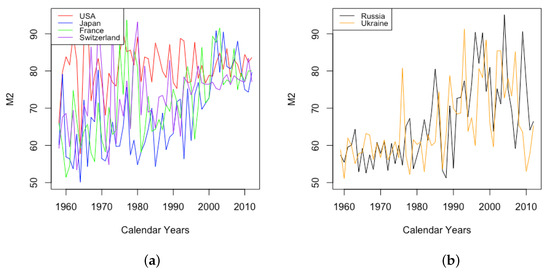
Figure 11.
(a) The age of fastest growth of the mortality acceleration factor across HLE countries. (b) The age of fastest growth of the mortality acceleration factor across ILE countries.
In both cases, the overall tendency is toward larger values, suggesting that contributed somewhat to mortality improvement in all countries.
The parameter is essentially flat, staying around the value 0.1 with occasionally spikes below this level, for all six countries over years when they all have data. The parameter is observed to stay flat or trend slightly upward for all six countries, with occasional spikes above the gradual trend (see Figure 12). The value of is consistently above for all six countries, although still usually less than 0.2. Intuitively, it is reasonable that age-dependent factors that accelerate mortality would have a lesser effect at younger ages and a stronger effect at old ages. Looking at older data, the flat nature of is observed in France all the way back to 1816, while in Switzerland, the value increased significantly between 1876 and 1960.
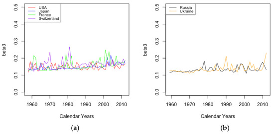
Figure 12.
(a) Level of the mortality acceleration factor at old ages across HLE countries. (b) Level of the mortality acceleration factor at old ages across ILE countries.
A plot of does not show a trend for any country/gender combination, except a trend downward for Ukrainian female data. An augmented Dickey–Fuller test provides the same conclusions—only the Ukrainian female dataset shows evidence of non-stationarity. However, an examination of the sample autocorrelations for the other datasets indicates positive autocorrelations at most lags, except for Japanese males and females. For France and Russia, there is enough data that the first few autocorrelations are significantly different from 0.
In summary, after 1950, for all the six countries, the growth rate function for the mortality caused by factors during adulthood and old ages has a stable mortality growth rate in young adulthood , a gradually increasing mortality growth rate in very old adulthood , and a gradual delay in the age of fastest increase , while the growth rate at that age is seen to remain stable, except for a decrease observed for Ukrainian females.
Mortality deceleration factor with parameters and
The mortality caused only by factors during adulthood and old age, , involves the mortality deceleration function . This would intuitively include the effect of technological advancements and other improvements in personal health and healthcare systems. For the DLGC, we chose the particular form of in Equation (9). This function takes on three main approximate levels: before age 65, between 65 and 85, and 1 above age 85. The change between two adjoining levels is logistic, the two changes occurring at ages 65 and 85, and beyond 85, the model assumes that , so that the parameter g will represent the limiting mortality from factors arising during old age. We intuitively view increases in or as mortality improvement, since such changes indicate a greater decelerating effect on mortality.
The value of was generally seen to trend upward for all countries for the complete period of available data, indicating that it consistently contributes to mortality improvement, as seen in the top panels of Figure 13. The bottom panel shows for French males and females. For both datasets, stays between 1 and 3.7 for the first century of data. Then, there is a gradual increase for both datasets, whose values still continue to stay close together. Starting in 1956, there is a sustained upward trend in the value of for females. While the value for males has also generally trended up since, with a couple of periods of retreat, starting with the 1950s, there is a marked difference between males and females, with seeming to contribute much more to mortality improvement for females than for males. This separation of the female and male curves occurs in all of the HLE countries at around the same time and will be discussed further in Section 3.3.
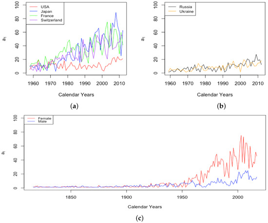
Figure 13.
(a) Mortality deceleration level before age 65 across HLE countries. (b) Mortality deceleration level before age 65 across ILE countries. (c) Mortality deceleration level before age 65 for France, male vs. female.
Plots of for HLE countries reveal either a trend upward or else an increase in variance, with the lowest values remaining near 1 in some years, but the maximum observed values increasing over time. Either situation is evidence that is contributing to mortality improvement. In ILE countries, there is another transition point after which the male and female values show sustained separation. In 1993 in Russia and 1995 in Ukraine, we see for the male data jump up to significantly higher levels and remain above the value for female data ever since, as depicted in Figure 14.
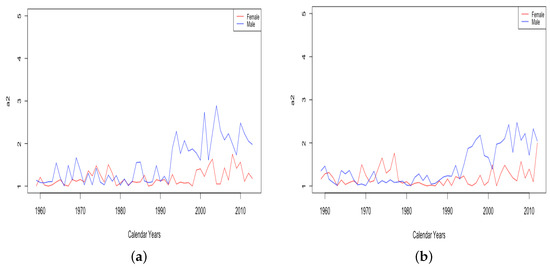
Figure 14.
(a) Mortality deceleration factor between ages 65 and 85 for Russia, male vs. female. (b) Mortality deceleration factor between ages 65 and 85 for Ukraine, male vs. female.
Comparing the levels of and , in all contexts, it is observed that is much greater than , so the beneficial factors that decelerate mortality have more of an effect at younger ages than older ages. This justifies the assumption that at very old ages, will be approximately 1.
Modal age at death calculated from fitted
After fitting the DLGC, we used the method described in Section 2.5 to calculate the modal age at death M from the fitted values of . Figure 15 shows the derived modal age at death M changing over years in each country, with HLE countries on the left and ILE countries on the right. An increasing M indicates mortality improvement, a result of synthesizing the improvement of the mortality from the youngest ages , the mortality from the teenage years , and the mortality from adulthood and old age .
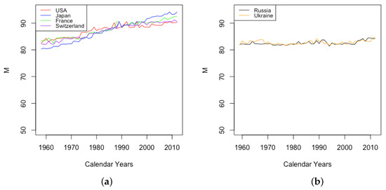
Figure 15.
(a) The modal age M for females in HLE countries. (b) The modal age M for females in ILE countries.
The HLE countries show increasing modal age at death, while the ILE countries have essentially stable values of M, except for a small increase starting in 2010. All countries had comparable values in 1959, but HLE countries now have considerably higher M than ILE countries. Separating by gender shows generally the expected gender gap, with modal age at death for females higher than that for males in the same country. The modal age at death for females was stable in Ukraine and increased in Russia, while the value has steadily decreased for Ukrainian males. In Russia, the value for males was stable at around 75 years until 1993, after which it dropped by several years, finally returning to stabilize around 75 years again in 2011.
3.3. Events and Inventions—Effects on Parameters
Some world events and developments have such an impact on mortality that their effects can be observed in time plots of the fitted parameters of the DLGC. These were mentioned in several places in previous sections:
- The effect of World Wars both on the goodness of fit of the model and on the value of , the limiting teenage mortality.
- The spike in in Switzerland in 1918, larger for males than females.
- The sudden and sustained drop in for females in all HLE countries, starting in 1949 in France, 1952 in the USA, 1953 in Switzerland, and less sudden in Japan, but trending down sharply beginning around 1950.
- The sudden and sustained increase for females of , the mortality deceleration factor for adults under 65, staring in 1950 in Switzerland and the USA, 1952 in France, and 1958 in Japan.
- The sudden and sustained increase for males of , the mortality deceleration factor for adults between 65 and 85, starting in 1993 in Russia and 1995 in Ukraine.
Our attribution of causes to these patterns is speculative and not scientific. Nevertheless, we think it is clear that Observation (1) is because of the World Wars. The spike is most evident in France, which saw many deadly battles in both wars; it is far larger in males than in females; it is far larger in the dataset of all males than just the dataset of civilian males. Examining all years of data for the total male population, the spikes are present in 1870–1871, 1914–1918, and 1940, 1943, and 1944. The first spike coincided with the Franco-Prussian War, and the others cover almost completely the periods of the World Wars. Switzerland stayed neutral through these wars, and we see no corresponding spike in the Swiss values of (see Figure 16).
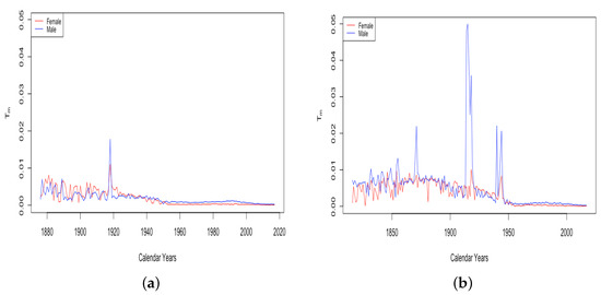
Figure 16.
(a) The limiting teenage mortality for Switzerland, male vs. female. (b) The limiting teenage mortality for France total population, male vs. female.
Item 2 above concerns the spike evidenced in the above graph of for Switzerland in 1918. A spike in this year is also observed in both male and female datasets in France, the only countries in our study with data going back that far. We speculate that this is because of the “Spanish Flu” pandemic, which was introduced to Europe by American soldiers in the spring of 1918. Two waves of the flu swept through Switzerland in 1918, infecting as much as 50% of the population and killing 6.2%. Part of the reason for the wide transmission is that the flu corresponded with the general strike. This involved 250,000 workers and also 90,000 soldiers mobilized to put down the strike. It is thought that this particular event contributed greatly to the spread of the virus around Switzerland, occurring as it did in the midst of the most deadly wave to spread through the country.
Items 3–5, by contrast, indicate a sustained improvement in mortality to one particular gender, occurring in multiple countries at approximately the same time. Both 4 and 5 indicate a significant improvement for females occurring mostly through the 1950s. Because is the limiting mortality caused by factors occurring in teenage years, while is the mortality deceleration factor in adults under age 65, there is an overlap in the age ranges involved with these parameters. In particular, we speculate that both of these developments indicate a sustained drop in mortality due to childbirth, which was the most common cause of death in teenage and young adult females before the advent of modern medicine (and is still the most common cause today in some developing countries).
Rather than a single factor, it is probable that several medical developments that occurred around the same time together led to the great decrease in mortality due to childbirth:
- The introduction of penicillin, which came into wide production in the mid-1940s and reduced death in many circumstances Sewell (1993). Deaths due to abortion in the USA dropped by 1950 to a fraction of their level in 1940 Gold (2003), perhaps due to the use of antibiotics to prevent infection after the procedure;
- Improvements in the healthcare environment during labor, including a huge increase in the percentage of births occurring in hospitals. In the USA in 1938, about half of births were occurring in hospitals, while by 1955, this had risen to 99 percent Sewell (1993);
- The widespread introduction of birth control pills starting in 1960.
Figure 17 shows the graph of for each of the HLE countries. (For the ILE countries, data begin in 1959, by which time, the separation between the male and female graphs is already evident.) Figure 18 shows the graph of for each of the countries. In each case, it is striking how similar the timing is of the separation between the curves, as well as the sustained nature of the separation.
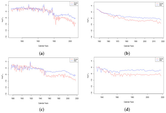
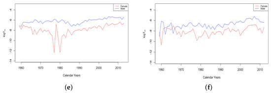
Figure 17.
(a) The log of limiting teenage mortality in France. (b) The log of limiting teenage mortality in Japan. (c) The log of limiting teenage mortality in Switzerland. (d) The log of limiting teenage mortality in the USA. (e) The log of limiting teenage mortality in Russia. (f) The log of limiting teenage mortality in Ukraine.
Figure 18.
(a) The log of mortality deceleration factor before age 65 in in France. (b) The log of mortality deceleration factor before age 65 in in Japan. (c) The log of mortality deceleration factor before age 65 in in Switzerland. (d) The log of mortality deceleration factor before age 65 in in the USA. (e) The log of mortality deceleration factor before age 65 in in Russia. (f) The log of mortality deceleration factor before age 65 in in Ukraine.
Finally, Item 5 indicates a significant improvement in the mortality deceleration factor between ages 65 and 85 for males in Russia and Ukraine, starting in the early 1990s (see Figure 14). We speculate here that this is related to the dissolution of the USSR and the end of the communist economic model in these countries a few years prior.
3.4. Use Observed Structure Change in Mortality to Choose Fitting Data in Forecasting
Section 3.3 demonstrated that the parameter interpretability of DLGC can reveal systematic structural changes in mortality patterns over time. When forecasting, the existence of such a change during the time interval of the training data casts doubt on the credibility of the data from before the change.
To test whether this idea had practical import for forecasting using DLGC, we noted the structural change in the limiting log teenage mortality around 1950 or a little after for females in Switzerland, the USA, France, and Japan, as described in Section 3.3, and we chose a training interval that placed the time of the change during the first 10 years of the training interval. We then cut the first ten years out of the training interval and fit the model a second time. Although the amount of training data was significantly reduced, we guessed we might see nonetheless an improvement in forecast accuracy because the period with the structural change had been removed. We performed the same experiment with Russia since the diagrams in Section 3.3 reveal that the log of teenage mortality in Russian females exhibited some spikes a little before 1980, and the spikes marked a transition from a trend that had been steadily decreasing to one that was steadily increasing. The training and forecast years for these data were several decades later than those used for the experiment on the four HLE countries.
The results of these experiments are presented in Table 10. The main body of the table shows pairs of columns—a white column and then a column with colors. Each cell in these columns shows the forecast error (expressed as an MSE) when forecasting a single year and comparing with that year’s realized mortality data from the HMD. The white columns use the full training set, while the colored columns use the truncated training set that excludes the noted structural change. Forecasts were made for each of the first ten years immediately following the training interval. Yellow cells indicate that the truncation idea has merit: in those cells, the forecast error using the truncated training set had decreased compared to the error when using the full dataset. Orange cells indicate the opposite.
Table 10.
DLGC 10-year-ahead forecasts’ accuracy is improved by fitting chosen data.
Table 11 shows a control for this experiment. After fitting the data for males from the same countries over the same time intervals, no major structural changes were observed in any parameter for France, Switzerland, and the USA. It seemed reasonable to use the male data from these countries as controls, since if older data are still reasonably credible, we would expect shrinking the training dataset to decrease forecast accuracy. The table supports this thinking.
Table 11.
DLGC 10-year-ahead forecasts’ accuracy in males as controls to Table 10.
These experiments demonstrate an advantage offered by a model based on highly interpretable parameters—the parameter plots can help the forecaster select a training set to improve forecasting accuracy. The dominance of yellow cells in the first table is evidence that training the model on data from before a structural change to forecast mortality for a period after the structural change is detrimental. The dominance of orange cells in the second table shows that otherwise cutting out the first ten years of a training dataset has a harmful effect on forecast accuracy (so that the dominance of yellow in the first table does not seem to be a result of just a significant lack of credibility in the data being removed because of the time lapse since it was recorded).
3.5. Life Expectancy Improvement and Gender Gap Quantitative Analysis
In this section, we use the fitted DLGC to give a quantitative analysis of life expectancy improvement over a chosen time period, and we analyze the life expectancy gap between genders for each country. We used the same life table techniques as used by HMD Wilmoth et al. (2007) to derive life expectancy at age x, denoted as , focusing only on , the life expectancy at birth.
We followed the same technique as used in de Beer and Janssen (2016) to decompose the change in life expectancy. In order to quantify the contribution from each parameter to life expectancy improvement, we began by specifying an order for the parameters and fixing country/gender and time interval. We fit the DLGC model to the specified country/gender for the first and final years of the time interval. Then, beginning with the model fitted to the earlier year’s data, we proceeded through the sequence of parameters, replacing the next parameter value by its value when the model is fit to the later year, while keeping other parameters unchanged. As each change was made, we determined the life expectancy estimated from the model using the updated values of the parameters. For example, to decompose the improvement in life expectancy at birth from year 1947 to 2019 in Japan, we may start our sequence of parameters with A followed by B. We fit the DLGC to the 1947 data for Japan and computed the life expectancy at birth . We then changed the value of A in the model to that produced by fitting DLGC instead to the 2019 data, leaving the other parameters fixed, and then recomputed using the fitted mortalities from this updated model. Then, we moved on to parameter B, replacing the value of B in the updated model with the value produced by fitting DLGC to 2019 data, keeping all other parameters unchanged, and recomputed . The change in after the first update is viewed as the contribution of A to the improvement of life expectancy at birth in this context, while the change in after the second update is viewed as the contribution from B. We proceeded through the parameters until, after the last update, the model being used was precisely the one obtained by fitting DLGC to the 2019 data.
There was a difference between the overall life expectancy change from our fitted model and the change in the life expectancy observed in the data. We label this difference as “unexplained”.
The ordering of the parameters we will use is: A, B, C, , k, z, , g, , , , , , . By changing only, we produce a contribution to the total life expectancy improvement from improved mortality at the earliest ages. The increase in life expectancy after changing is regarded as the contribution from mortality improvement during teenage years. Finally, we changed the remaining parameters, and the change in life expectancy varying is regarded as the contribution from adulthood and old age. We ran this quantitative analysis for each of the four HLE countries, in each case over the total interval of available data. The results are summarized in Table 12. We then ran the analysis over the largest time interval (1959–2013) for which all countries, both HLE and ILE, have data, using data for females only. The result is summarized in Table 13. In both tables, the incremental change in life expectancy at birth is given first for the raw data, then the parts explained and unexplained by the fitted model, and then, broken down into the three age categories, singling out in particular the contributions from the parameters A, , g and .
Table 12.
Life expectancy improvement quantitative analysis over all available years for 4 HLE countries.
Table 13.
Female life expectancy improvement quantitative analysis during years 1959 to 2013 for 6 countries.
As is shown by the life tables, there is an overall increase in life expectancy at birth in all countries and for both genders, with sightly less total improvement for males than females. The detailed quantitative analysis in the table reveals more: the life expectancy improvement contribution from the earliest ages and teenage years in males is usually near or even higher than that of females. By contrast, the contribution to life expectancy improvement from adulthood and old ages is higher for females than males and is a larger effect than the contributions from the lower age groups. This dominating effect of the contribution from improvement in adulthood and old age then leads to the overall life expectancy improvement being larger for females than males.
The life expectancy at birth in Switzerland and France has improved by more than 40 years from the 19th Century to 2018, with most of the improvement happening in the 20th Century. From quantitative analysis (not shown), French females exhibited an increase of 38.54 years of life expectancy between 1900 to 2018, while Swiss females exhibited an increase of 35.44 years over the same period.
Table 13 reveals, as expected, that the four HLE countries saw much higher increases in total life expectancy at birth than the two ILE countries. It also reveals that the contribution gap between the four HLE countries and two ILE countries from the earliest ages and teenage years are very small. Thus, the main reason for the HLE countries’ greater overall improvement is their much greater improvement within adulthood and old ages.
Among the four HLE countries through 1959 to 2013, the quantitative analysis reveals that the main contribution to improved life expectancy is from adulthood and old age. Furthermore, for the six countries studied, the ordering of countries by overall improvement in life expectancy matches the order when looking just at the contribution to improvement from adulthood and old ages. Japan shows the most impressive mortality improvement in every age category, and indeed, it had the lowest life expectancy at birth in 1959 and the highest by 2013.
Finally, we note that it appears that for the simpler parts of the model, and , representing the contribution to mortality from the youngest children and from teenagers, the improvement in life expectancy is explained mostly by changes just in the parameters A and . By contrast, the parameters and g representing the main processes in the logistic model for do not account for most of the increased life expectancy in most cases. The value of g can actually contribute to decreased life expectancy, and this is especially observed in the Russian and Ukrainian female data. However, the contribution from the simultaneous increase in the age more than compensates for the decrease in these cases, giving a quantitative view of compression at work.
Overall, the inability of g and to explain most of the life expectancy improvement in adulthood, as well as the dominating effect of the contribution to improvement from this age group lends further credibility to the choices made in the framework introduced in this paper. It seems the new factors and serve a substantive role in the model and that the particular choices for and made for DLGC were effective in capturing some of the nuance in mortality among adults.
4. Conclusions
The DLGC introduced in this paper uses a deterministic form to describe mortality features across ages and applies stochastic processes to model and forecast changing mortality over time. We used the model to fit and forecast the mortality of France, Switzerland, Japan, the USA, Russia, and Ukraine, for both genders.
At the age-specific level, DLGC produces smooth fits and predictions across age and provides insights about mortality structure and development with good interpretability. The yearly fitting results for all six countries are excellent through two centuries of data for female and male and for both HLE countries and ILE countries. Considering future mortality, DLGC creates accurate in-sample forecasts, especially the 10-year-ahead forecasts, which almost always outperform the logit-binomial Lee–Carter model in the R package StMoMo Villegas et al. (2018) for all six countries and both genders.
The DLGC parameters have clear mortality interpretations, and their time plots show stable tendencies that match known demographic characteristics and trends. In addition, the plots can reveal mortality structural changes such as mortality compression at the age-specific level and temporary or persistent changes in mortality trends caused by transitions in major causes of death (see Section 3.3). The structural change revealed by the plots can also suggest appropriate intervals of data to train the model (see Section 3.4). Furthermore, the plots can suggest an appropriate stochastic model for each parameter. In addition, the contribution of each parameter in life expectancy improvement was analyzed quantitatively.
The mortality framework introduced in Equation (7) depends on two age-specific functions, one for mortality-accelerating factors and one for mortality-decelerating factors. DLGC is an exemplar of the framework created by specifying those two functions, but the framework can be applied to different populations by changing the functions. For example, DLGC performs better for HLE countries than ILE countries, and we suspect that that is because we chose the functions based on the population features of HLE countries. In future research, we plan to explore other choices of the functions that better fit ILE and also to study low life expectancy countries.
To forecast with DLGC, we fit parameters over a given time interval with respect to the original (age-specific) model and assumed that their future values followed ARIMA time series. In doing so, our primary goal was to show that parameter plots can identify real structural changes in mortality patterns and that strategic choices in training data that avoid such changes improve forecasting.
However, the simple approach of forecasting each parameter time series using ARIMA does not capture correlation among the series. In future research, we plan to study in more depth how such relationships impact forecasting fit, as well as parameter interpretations. We also hope to use parameter time plots to revise our forecasting model to include stochastic and deterministic time-varying parameters in the age-specific component. The model would then have time-varying parameters and age-specific parameters and would have fewer parameters than the DLGC forecasting model does.
[custom]
Author Contributions
Conceptualization: W.F. and B.R.S.; methodology: W.F., B.R.S. and P.B.; software: W.F. and S.D.; validation: S.D. and B.R.S.; formal analysis: W.F.; investigation: W.F. and S.D.; resources: publicly available data from Human Mortality Database (HMD); data curation: HMD data are ready-to-use; writing—original draft preparation: W.F. and B.R.S.; writing—review and editing: W.F., B.R.S. and P.B.; supervision: W.F. and P.B.; project administration: W.F. and P.B.; funding acquisition: P.B. All authors have read and agreed to the published version of the manuscript.
Funding
This research received no external funding.
Institutional Review Board Statement
Not applicable.
Informed Consent Statement
Not applicable.
Data Availability Statement
Data available in a publicly accessible repository that does not issue DOIs. Publicly available datasets were analyzed in this study. These data can be found here: Human Mortality Database. University of California, Berkeley (USA), and Max Planck Institute for Demographic Research (Germany). Available at www.mortality.org or www.humanmortality.de (data downloaded on 15 July 2021).
Conflicts of Interest
The authors declare no conflict of interest.
Notes
| 1 | The data are period life tables from Human Mortality Database (n.d.), either female, male, or total. France has both data for the civilian population and the total population. |
| 2 | We use French civilian data instead of French total population data, since the DLGC generally provides a better fit to civilian data. |
References
- Bardoutsos, Anastasios, Joop de Beer, and Fanny Janssen. 2018. Projecting delay and compression of mortality. Genus 74: 17. [Google Scholar] [CrossRef]
- Blackburn, Craig, and Michael Sherris. 2013. Consistent dynamic affine mortality models for longevity risk applications. Insurance: Mathematics and Economics 53: 64–73. [Google Scholar] [CrossRef]
- Booth, Heather, and Leonie Tickle. 2008. Mortality Modelling and Forecasting: A Review of Methods. Annals of Actuarial Science 3: 3–43. [Google Scholar] [CrossRef]
- Booth, Heather, John Maindonald, and Len Smith. 2002. Applying Lee–Carter under conditions of variable mortality decline. Population Studies 56: 325–36. [Google Scholar] [CrossRef] [PubMed]
- Burger, Oskar, Annette Baudisch, and James W. Vaupel. 2012. Human mortality improvement in evolutionary context. Proceedings of the National Academy of Sciences USA 109: 18210–14. [Google Scholar] [CrossRef] [Green Version]
- Callot, Laurent, Neils Haldrup, and Marlene Kallestrup-Lamb. 2016. Deterministic and stochastic trends in the Lee–Carter mortality model. Applied Economics Letters 23: 486–93. [Google Scholar] [CrossRef] [Green Version]
- Carriere, Jacques F. 1992. Parametric models for life tables. Transactions of Society of Actuaries 44: 77–99. [Google Scholar]
- Continuous Mortality Investigation Bureau. 2006. Stochastic Projection Methodologies, Further Progress and p-Spline Model Features, Example Results and Implications. Working Paper 20. London: The Faculty of Actuariaes and Institute of Actuaries. [Google Scholar]
- de Beer, Joop, and Fanny Janssen. 2016. A new parametric model to assess delay and compression of mortality. Population Health Metrics 14: 46. [Google Scholar] [CrossRef] [Green Version]
- Gao, Huan, Rogemar Mamon, Xiaoming Liu, and Anton Tenyakov. 2015. Mortality modelling with regime-switching for the valuation of a guaranteed annuity option. Insurance: Mathematics and Economics 63: 108–20. [Google Scholar] [CrossRef]
- Gold, Rachel B. 2003. Lessons from before Roe: Will past be prologue? Guttmacher Report on Public Policy 5: 1–4. [Google Scholar]
- Gylys, Rokas, and Jonas Šiaulys. 2019. Revisiting Calibration of the Solvency II Standard Formula for Mortality Risk: Does the Standard Stress Scenario Provide and Adequate Approximation of Value-at-Risk? Risks 7: 58. [Google Scholar] [CrossRef] [Green Version]
- Gylys, Rokas, and Jonas Šiaulys. 2020. Estimation of Uncertainty in Mortality Projections Using State-Space Lee–Carter Model. Mathematics 8: 1053. [Google Scholar] [CrossRef]
- Hannerz, Harold. 2001. Presentation and derivation of a five-parameter survival function intended to model mortality in modern female populations. Scandinavian Actuarial Journal, 176–87. [Google Scholar] [CrossRef]
- He, Lingyu, Fei Huang, Jianjie Shi, and Yangrong Yang. 2021. Mortality forecasting using factor models: Time-varying or time-invariant factor loadings? Insurance: Mathematics and Economics 98: 14–34. [Google Scholar] [CrossRef]
- Heligman, Larry, and John Pollard. 1980. The age pattern of mortality. Journal of the Institute of Actuaries 107: 49–80. [Google Scholar] [CrossRef]
- Human Life Table Database. n.d. Available online: Https://www.lifetable.de/cgi-bin/country.php?code=zaf (accessed on 20 March 2022).
- Human Mortality Database. n.d. University of California, Berkeley (USA), and Max Planck Institute for Demographic Research (Germany). Available online: www.mortality.org (accessed on 15 July 2021).
- Hyndman, Rob J., and Yeasmin Khandakar. 2008. Automatic time series forecasting: The forecast package for R. Journal of Statistical Software 26: 1–22. [Google Scholar]
- Ignatieva, Katja, Andrew Song, and Jonathan Ziveyi. 2016. Pricing and hedging of guaranteed minimum benefits under regime-switching and stochastic mortality. Insurance: Mathematics and Economics 70: 286–300. [Google Scholar]
- Kannisto, Väinö. 1994. Development of Oldest-Old Mortality, 1950–1990: Evidence from 28 Developed Countries. Odense: Odense University Press. [Google Scholar]
- Lee, Ronald D., and Lawrence R. Carter. 1992. Modeling and Forecasting U.S. Mortality. Journal of the American Statistical Association 87: 659–71. [Google Scholar] [CrossRef]
- Lee, Ronald D., and Timothy Miller. 2001. Evaluating the performance of the lee-carter method for forecasting mortality. Demography 38: 537–49. [Google Scholar] [CrossRef] [PubMed]
- Lin, X. Sheldon, and Xiaoming Liu. 2007. Markov Aging Process and Phase-Type Law of Mortality. North American Actuarial Journal 11: 92–109. [Google Scholar] [CrossRef]
- McNown, Robert, and Andrei Rogers. 1989. Forecasting mortality: A parameterized time series approach. Demography 26: 645–60. [Google Scholar] [CrossRef] [PubMed]
- Milidonis, Andreas, Yijia Lin, and Samuel H. Cox. 2011. Mortality Regimes and Pricing. North American Actuarial Journal 15: 266–89. [Google Scholar] [CrossRef]
- Mullen, Katherine M., David Ardia, David L. Gil, Donald Windover, and James Cline. 2011. DEoptim: An R Package for Global Optimization by Differential Evolution. Journal of Statistical Software 40: 1–26. [Google Scholar] [CrossRef] [Green Version]
- Njenga, Carolyn Ndigwako, and Michael Sherris. 2020. Modeling mortality with a Bayesian vector autoregression. Insurance: Mathematics and Economics 94: 40–57. [Google Scholar] [CrossRef]
- Perks, Wilfred. 1932. On some experiments in the graduation of mortality statistics. Journal of the Institute of Actuaries 63: 12–57. [Google Scholar] [CrossRef]
- Pongou, Roland. 2013. Why is infant mortality higher in boys than in girls? A new hypothesis based on preconception environment and evidence from a large sample of twins. Demography 50: 421–44. [Google Scholar] [CrossRef]
- R Core Team. 2021. R: A Language and Environment for Statistical Computing. Vienna: R Foundation for Statistical Computing, Available online: Https://www.R-project.org/ (accessed on 31 December 2021).
- Renshaw, Arthur E., and Steven Haberman. 2003. Lee–Carter mortality forecasting with age-specific enhancement. Insurance: Mathematics and Economics 33: 255–72. [Google Scholar] [CrossRef]
- Renshaw, Arthur E., and Steven Haberman. 2006. A cohort-based extension to the Lee–Carter model for mortality reduction factors. Insurance: Mathematics and Economics 38: 556–70. [Google Scholar] [CrossRef]
- Rogers, Andrei, and Friedrich Planck. 1983. MODEL: A General Program for Estimating Parametrized Model Schedules of Fertility, Mortality, Migration, and Marital and Labor Force Status Transitions. IIASA Working Paper. Available online: https://pure.iiasa.ac.at/id/eprint/2210/ (accessed on 31 December 2021).
- Schrager, David F. 2006. Affine stochastic mortality. Insurance: Mathematics and Economics 38: 81–97. [Google Scholar] [CrossRef] [Green Version]
- Sewell, Jane Eliot. 1993. Cesarean section—A brief history. A Brochure to Accompany an Exhibition on the History of Cesarean Section at the National Library of Medicine Part 3 30. [Google Scholar]
- Sharrow, David, Samuel J. Clark, Mark Collinson, Kathleen Kahn, and Stephen Tollman. 2013. The Age-Pattern of Increases in Mortality Affected by HIV: Bayesian Fit of the Heligman–Pollard Model to Data from the Agincourt HDSS Field Site in Rural Northeast South Africa. Demographic Research 29: 1039–96. [Google Scholar] [CrossRef] [PubMed] [Green Version]
- Shen, Yang, and Tak Siu. 2013. Longevity bond pricing under stochastic interest rate and mortality with regime-switching. Insurance: Mathematics and Economics 52: 114–23. [Google Scholar] [CrossRef]
- Siler, William. 1979. Competing-Risk Model for Animal Mortality. Ecology 60: 750–57. [Google Scholar] [CrossRef]
- SriDaran, Dilan, Michael Sherris, Andrés M. Villegas, and Jonathan Ziveyi. 2022. A group regularization approach for constructing generalized age-period-cohort mortality projection models. ASTIN Bulletin 52: 247–89. [Google Scholar] [CrossRef]
- Tuljapulkar, Shripad, Nan Li, and Carl Boe. 2000. A universal pattern of mortality decline in the G7 countries. Nature 405: 789–92. [Google Scholar] [CrossRef]
- Villegas, Andrés M., Pietro Millossovich, and Vladimir K. Kaishev. 2018. StMoMo: An R Package for Stochastic Mortality Modeling. Journal of Statistical Software 84: 1–38. [Google Scholar] [CrossRef] [Green Version]
- Wilmoth, John R., Kirill F. Andreev, Dmitri Jdanov, and Dana A. Glei. 2007. Methods Protocol for the Human Mortality Database. Berkeley: University of California, Berkeley, and Max Planck Institute for Demographic Research, Rostock. [Google Scholar]
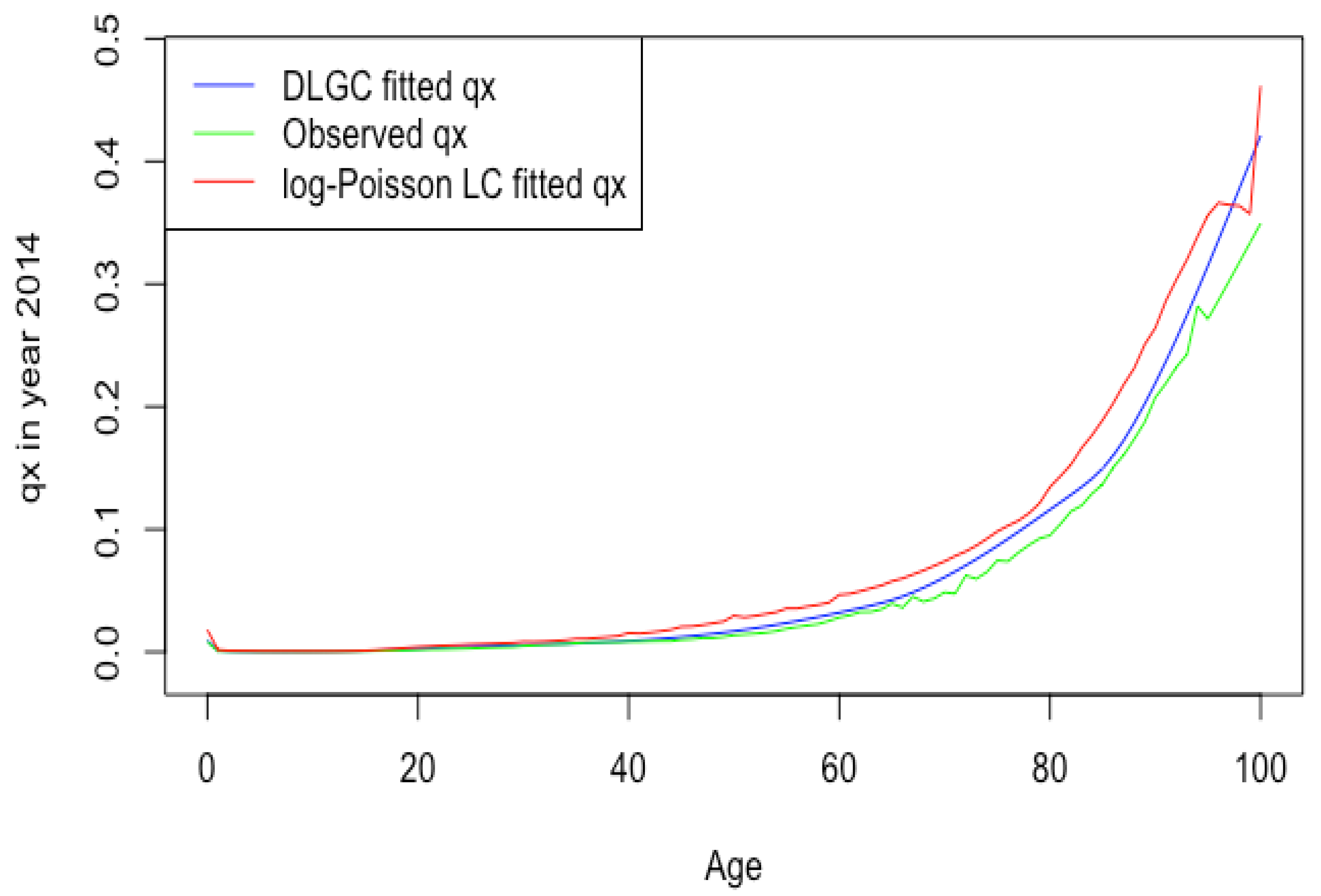
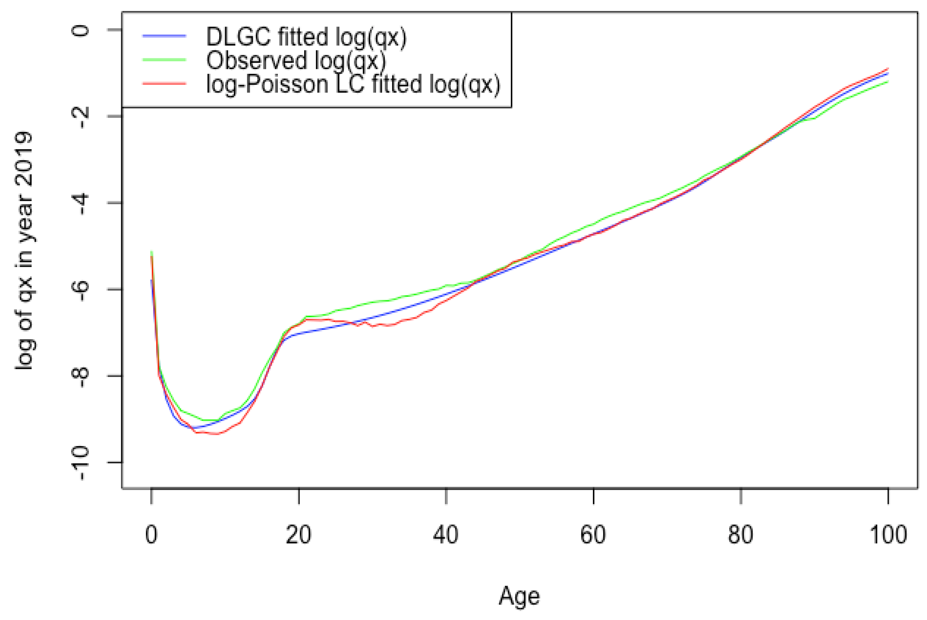
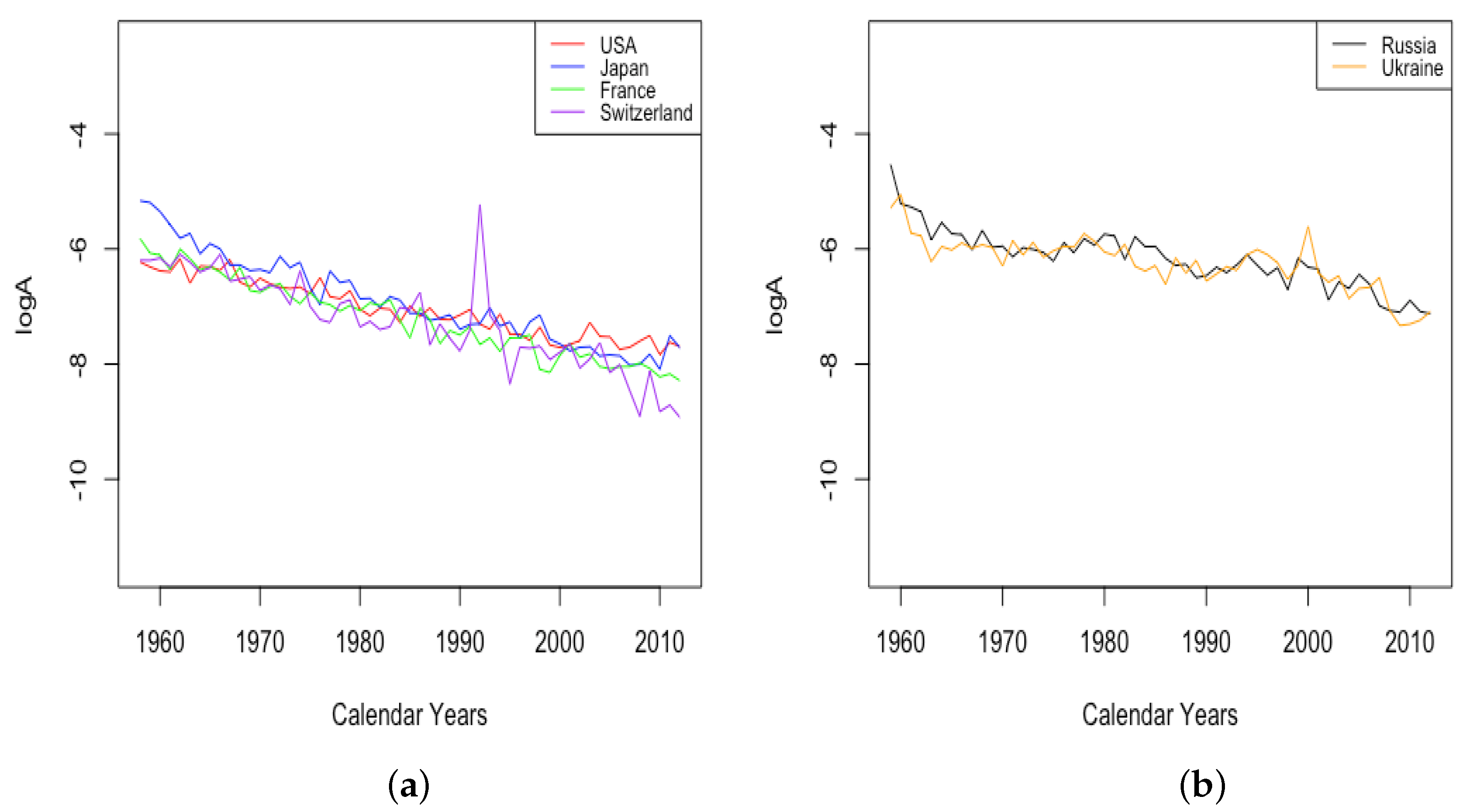
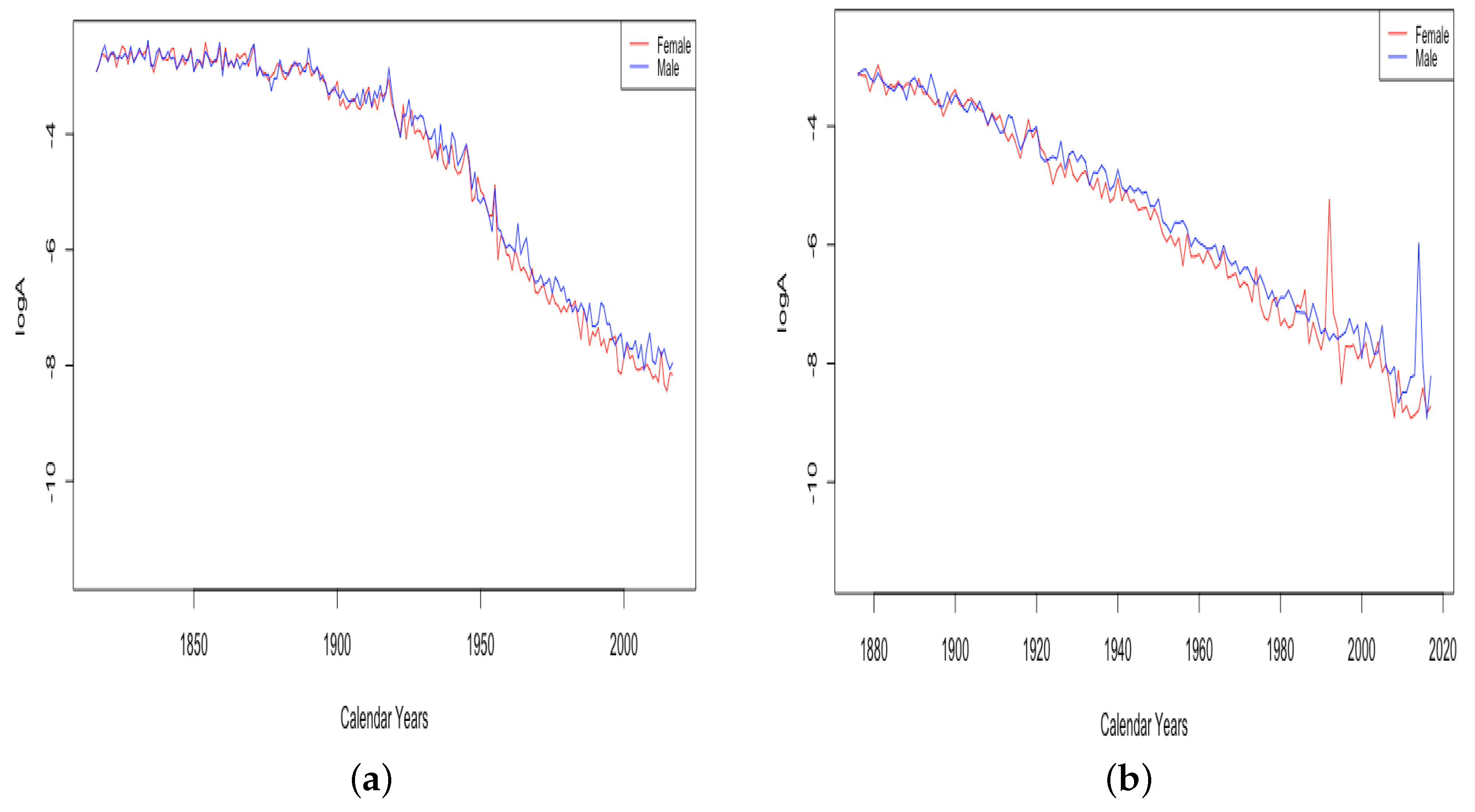
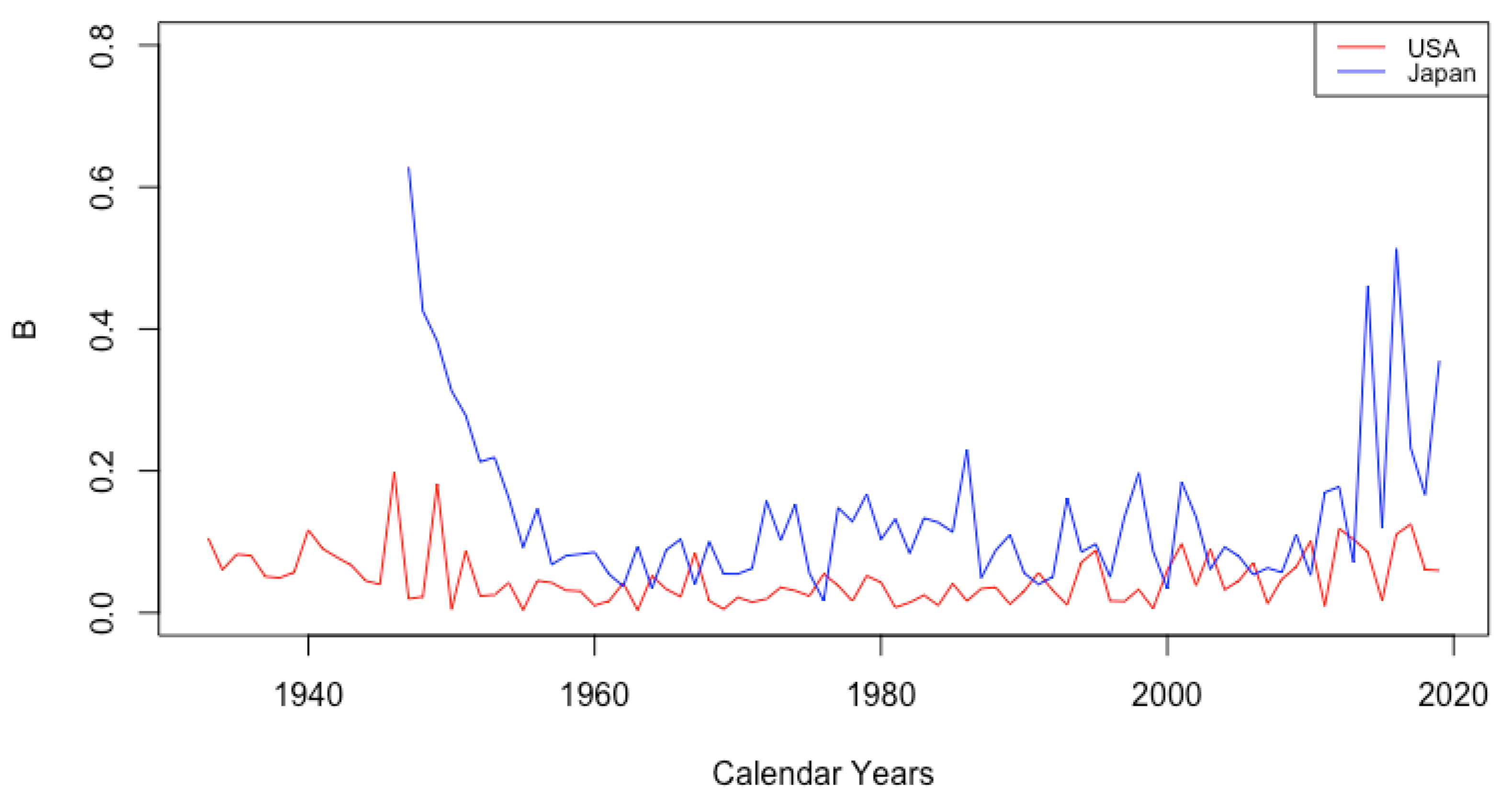
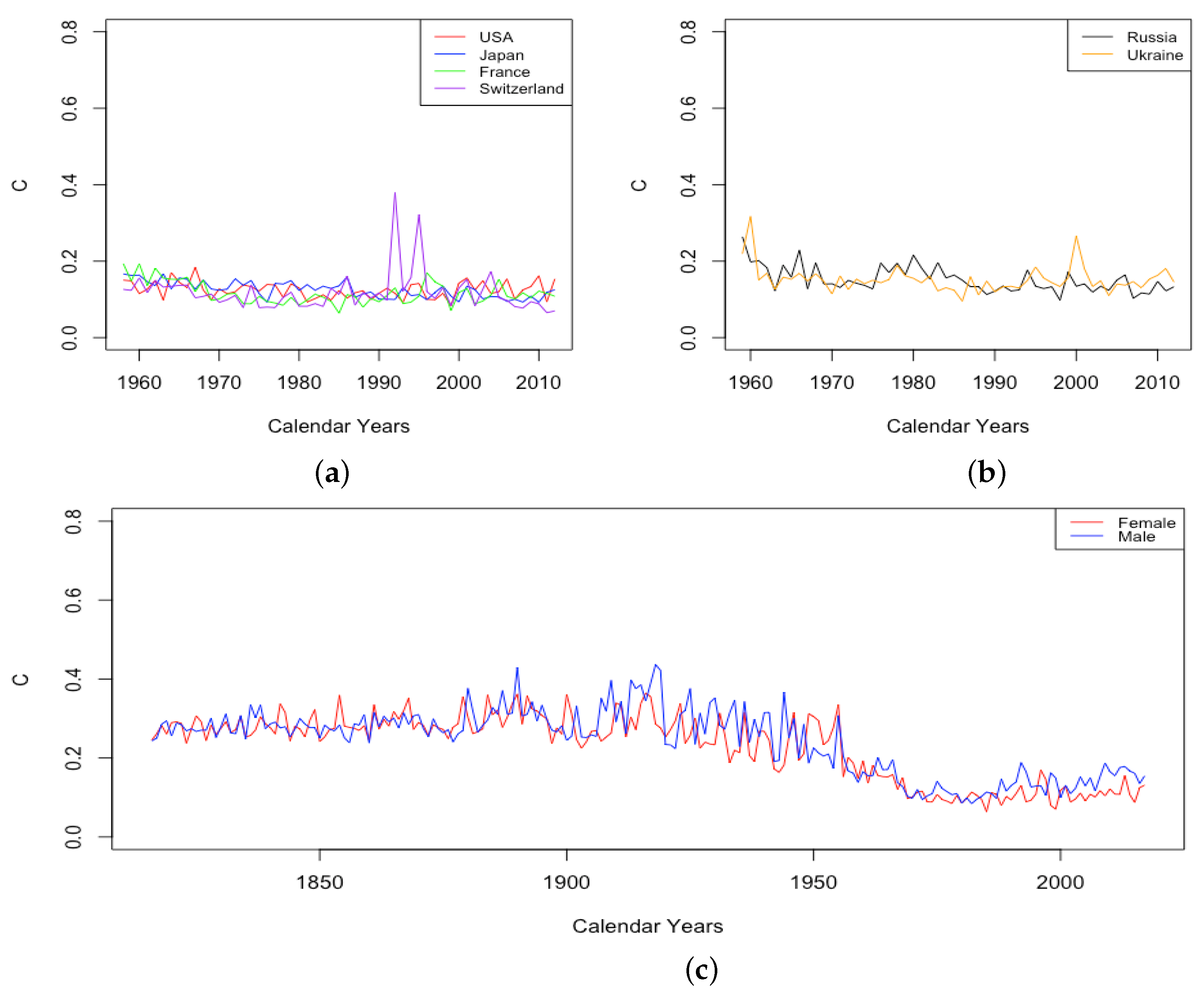
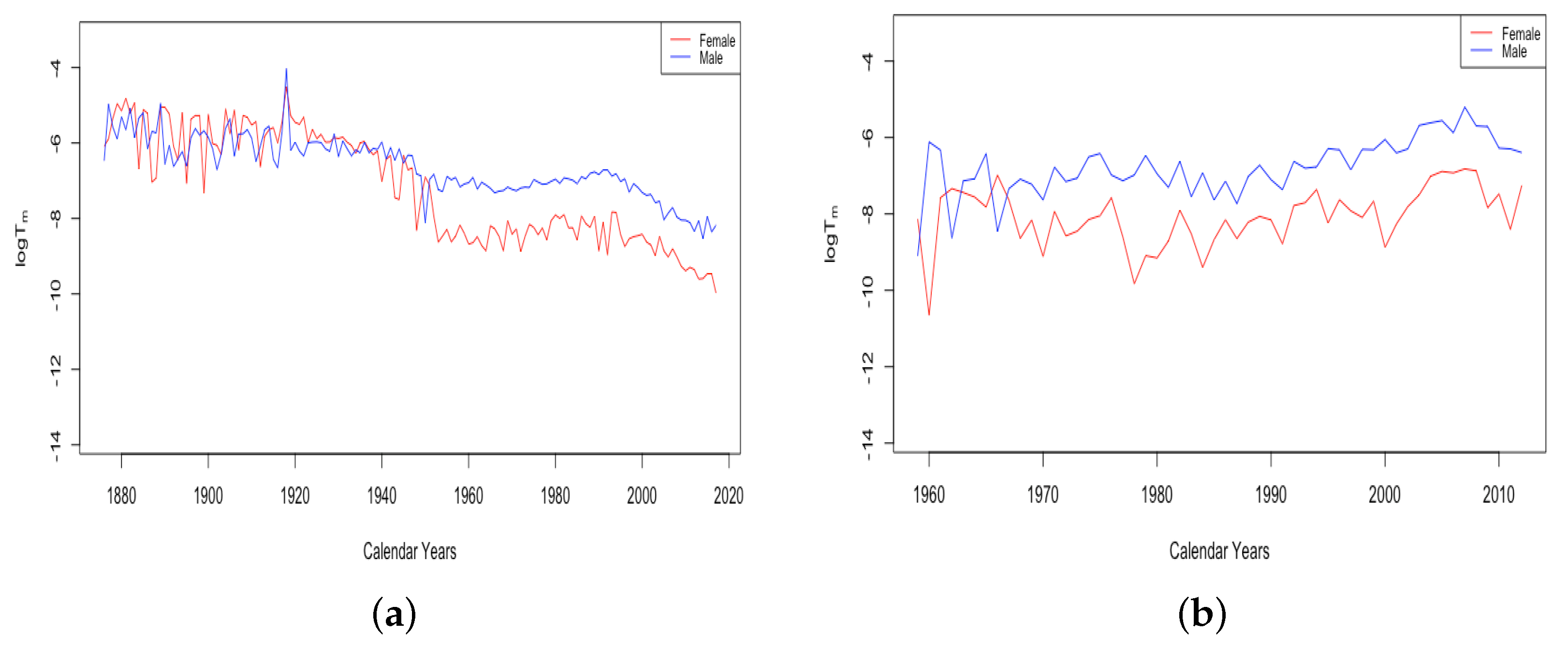

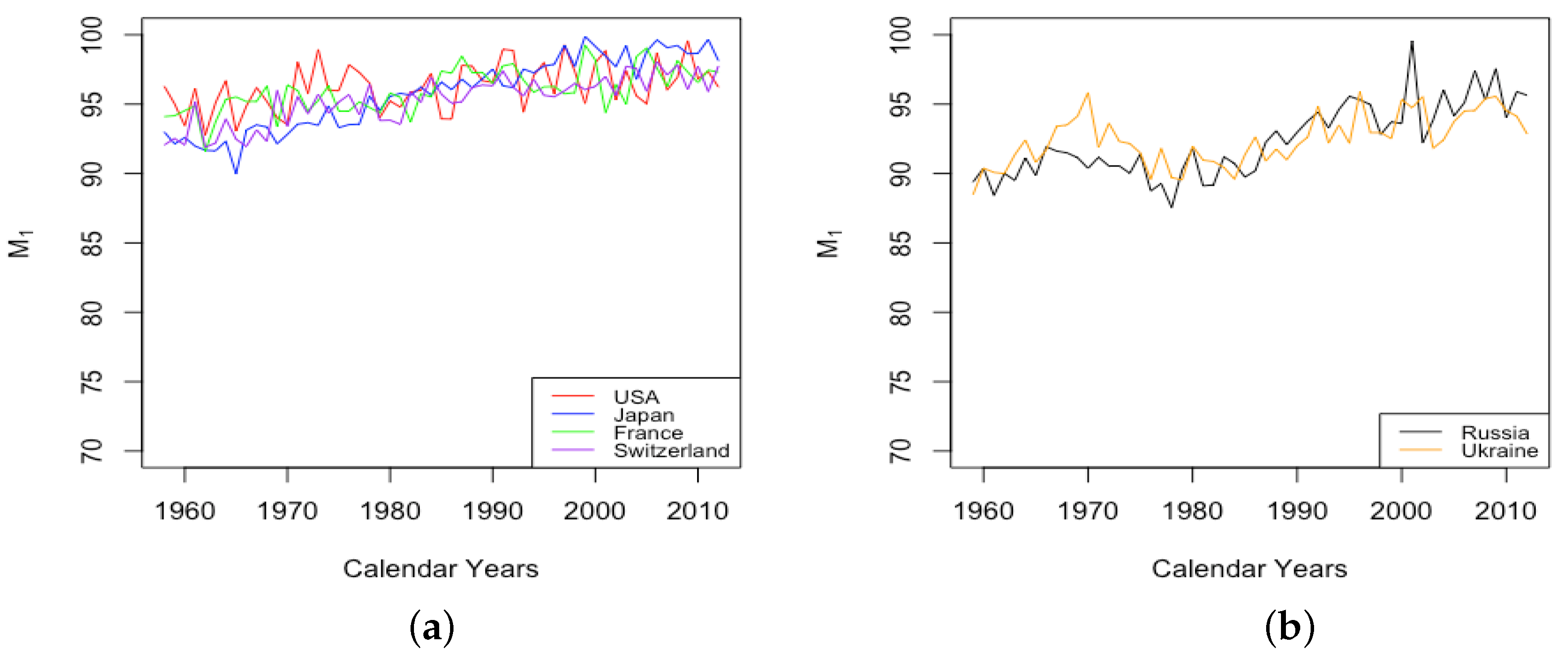


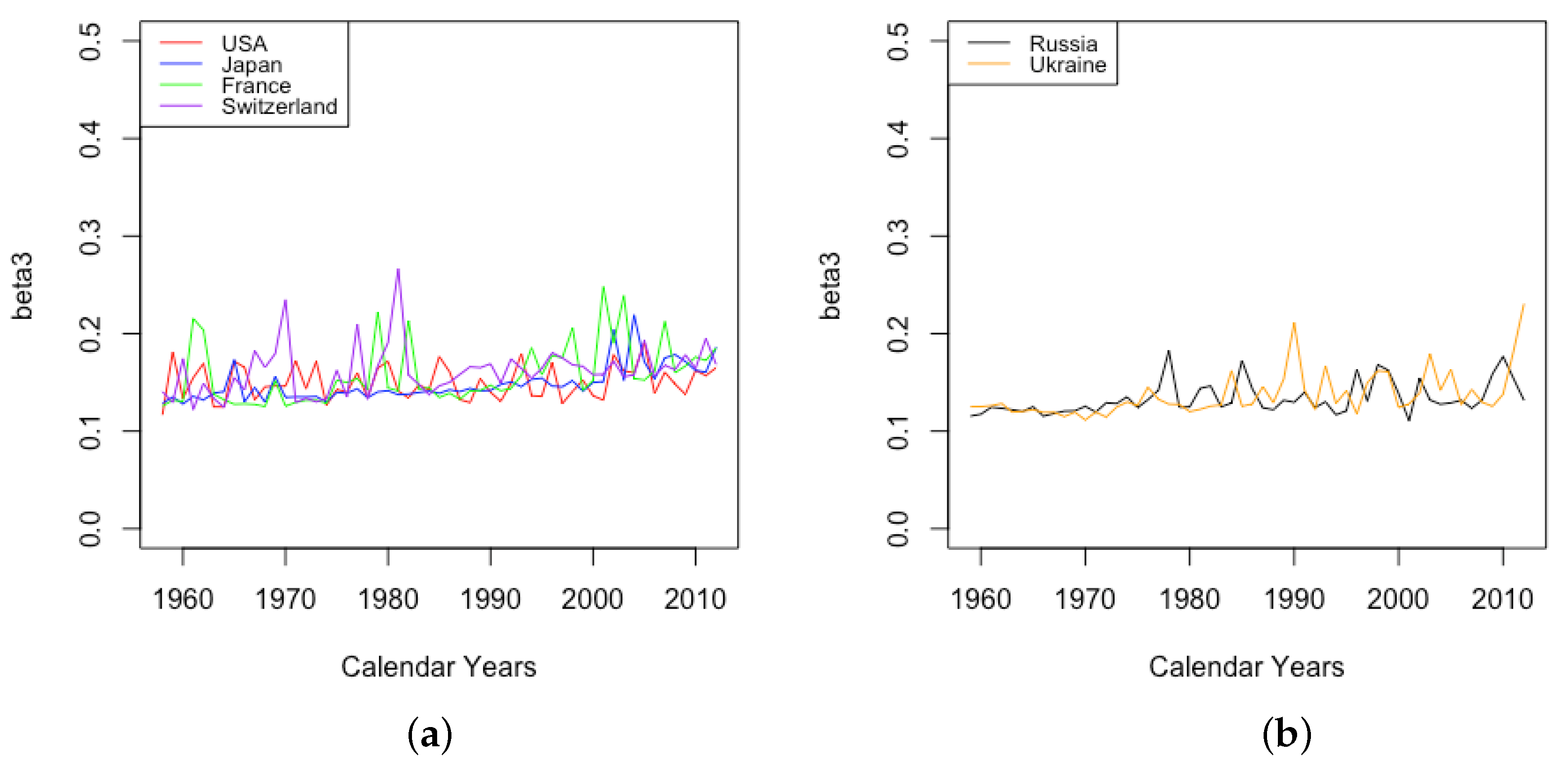
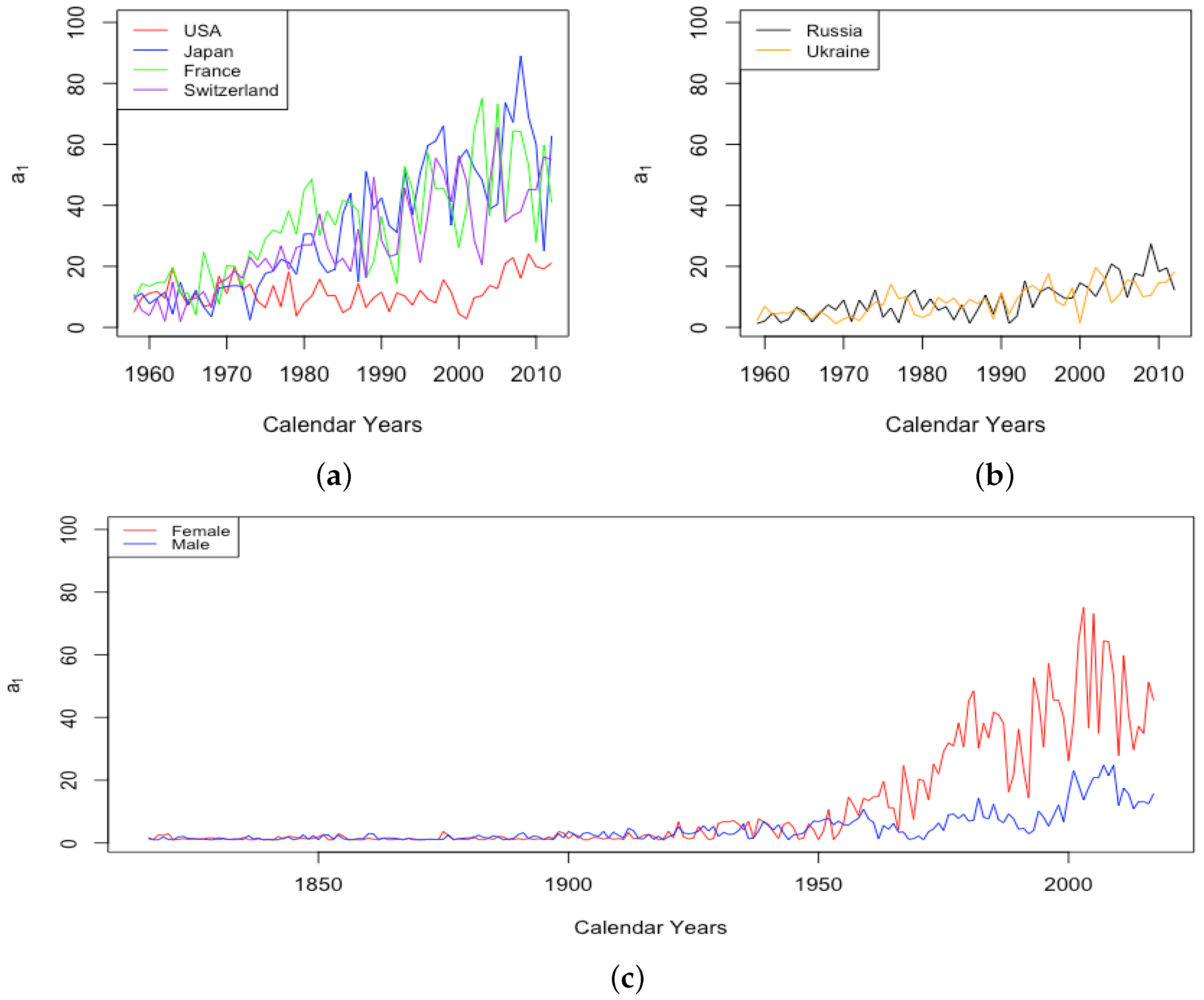
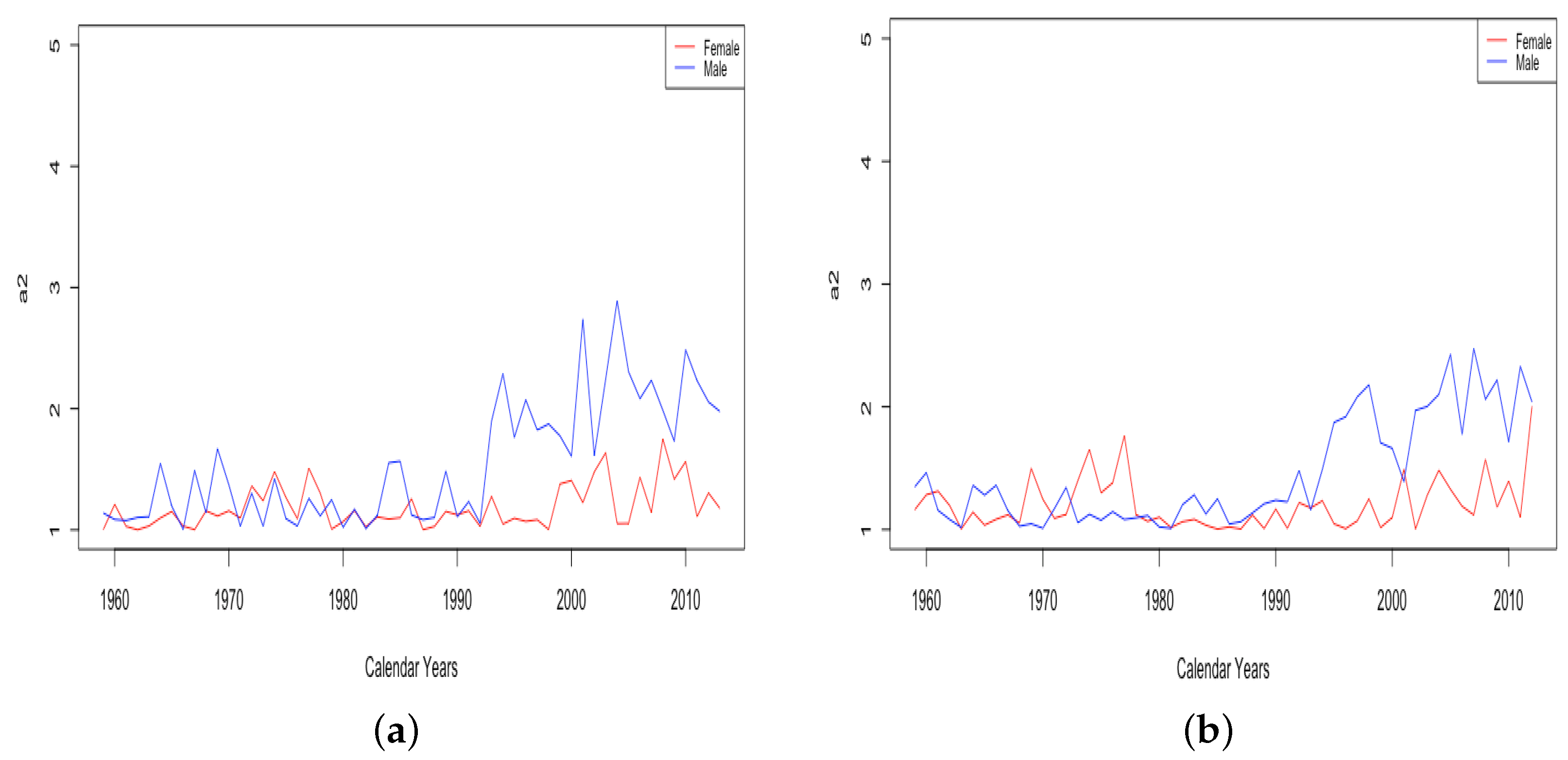
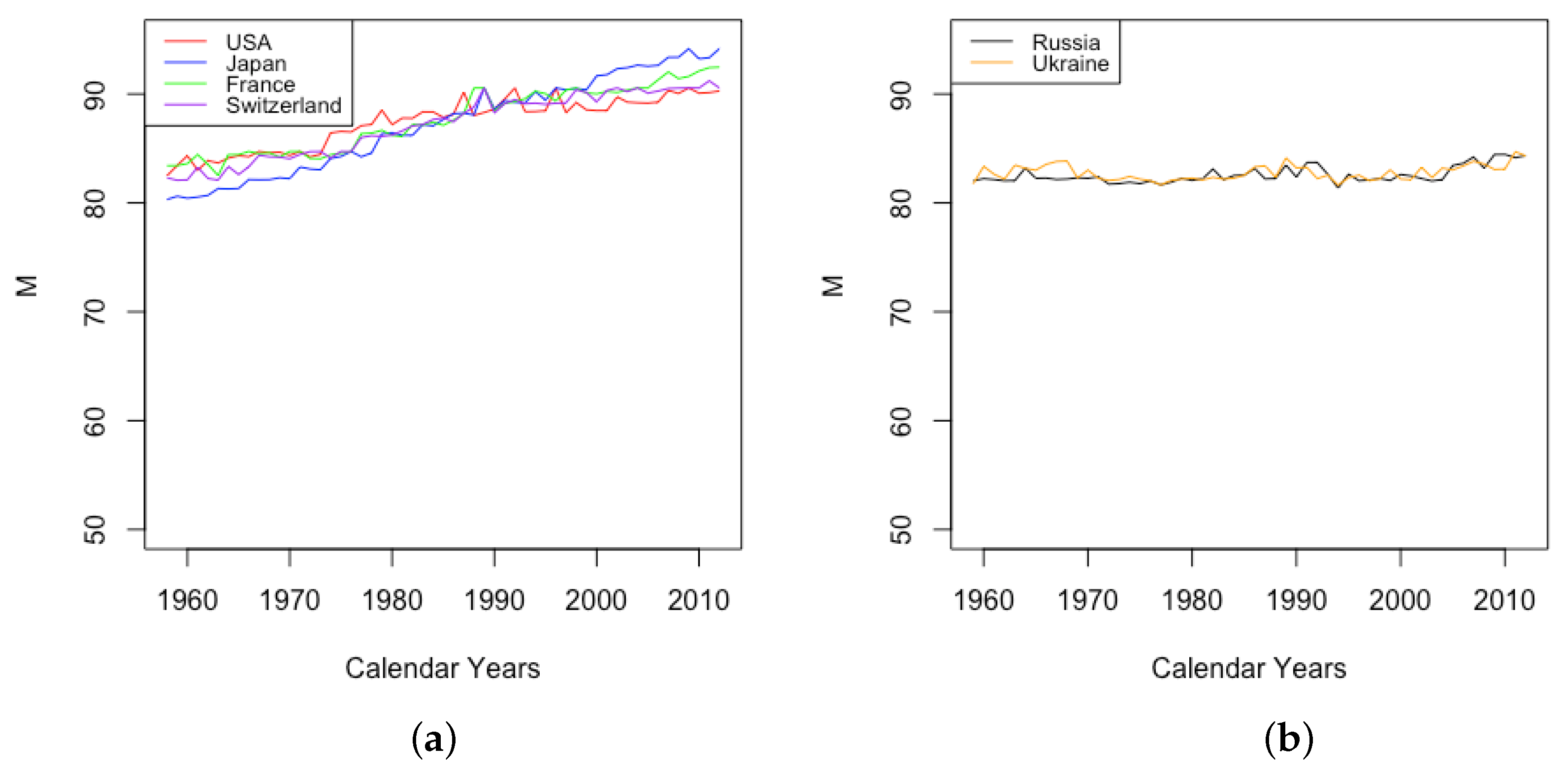
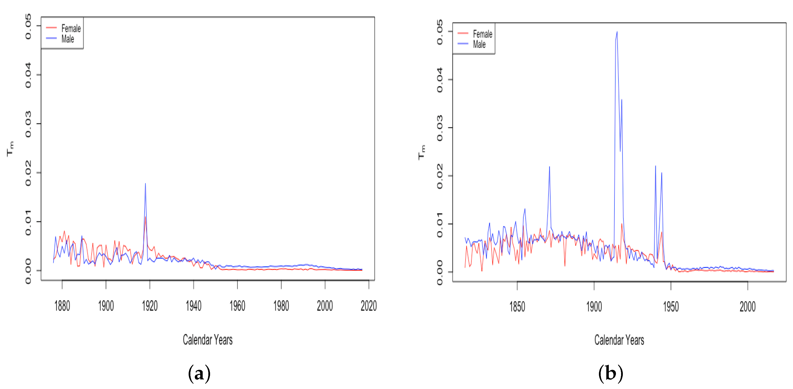

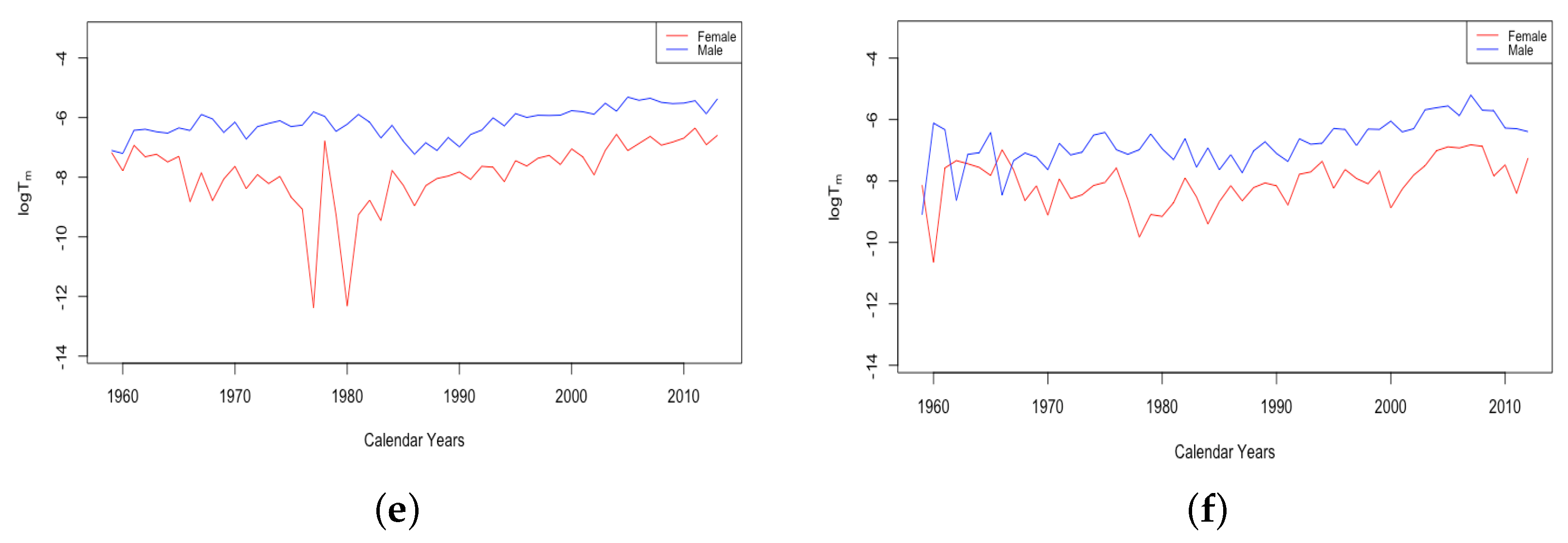
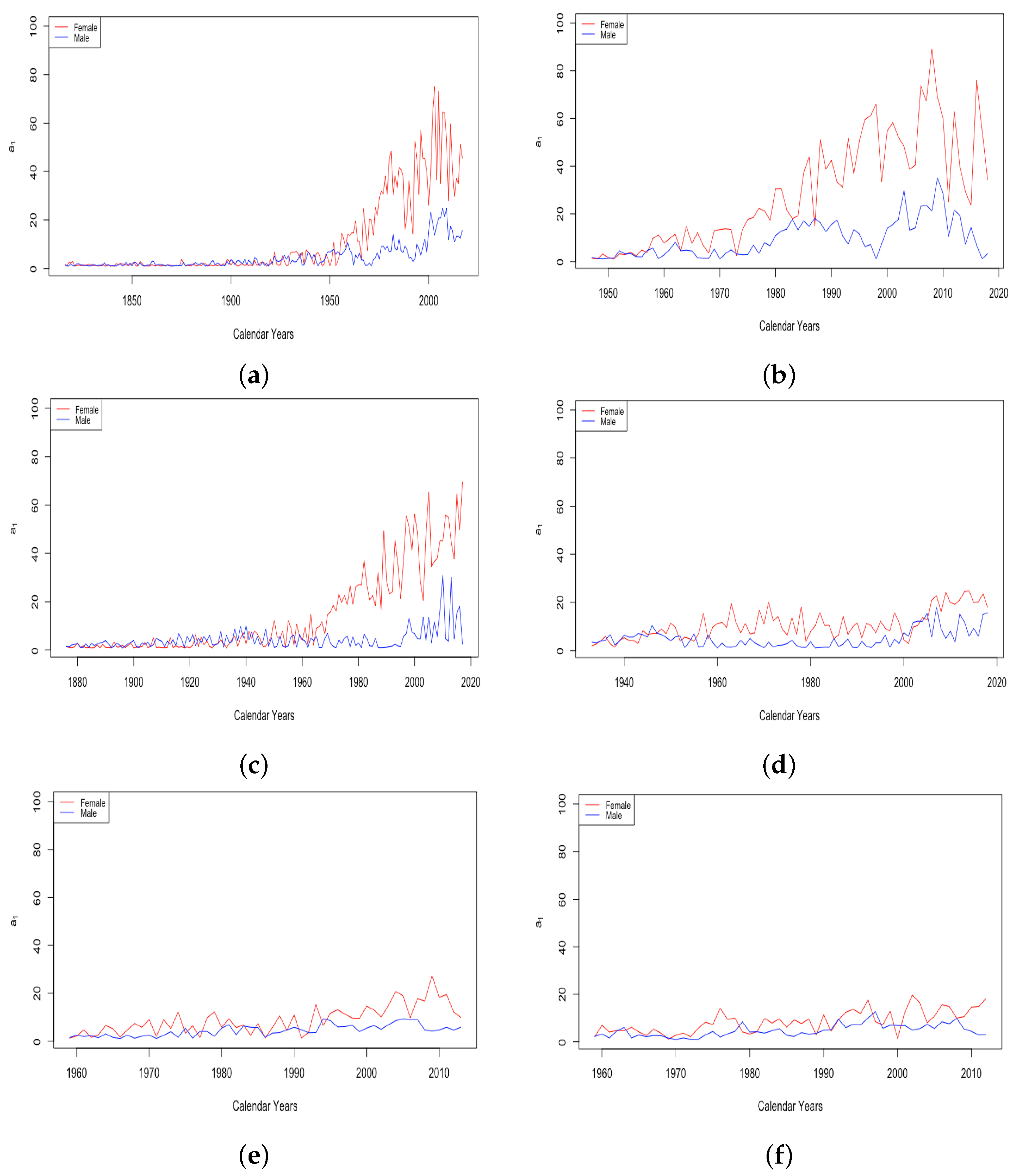
Publisher’s Note: MDPI stays neutral with regard to jurisdictional claims in published maps and institutional affiliations. |
© 2022 by the authors. Licensee MDPI, Basel, Switzerland. This article is an open access article distributed under the terms and conditions of the Creative Commons Attribution (CC BY) license (https://creativecommons.org/licenses/by/4.0/).