Abstract
The aim of this work is to introduce an innovative methodology for performing risk attribution within a multifactor risk framework. We applied this analysis to the assessment of systemic, climate, and geopolitical risks relative to a representative sample of Eurozone banks between 2011 and 2022. Comparing the results to the output of a bivariate approach, we found that contemporaneous tail crises generate combined equity losses exceeding partial analysis estimates. We then attributed the combined risk to each factor and to the effect of their interaction by employing our proposed frequency-based approach. For our computations, we used multivariate GARCH, Monte Carlo simulations, and a suite of Eurozone-specific factors. Our results show that total combined risk is on average 18% higher than traditional systemic risk estimates, that climate risk more than doubled in our period of analysis, and that geopolitical risk surged to over 5% of total combined risk. Our climate risk estimate is in line with the results of the 2022 European Central Bank climate stress test, and our geopolitical risk measure shows a positive correlation with the GPRD and Threats index.
1. Introduction
All banks are subject to specific risks that require regulatory capital: credit risk, market risk, and operational risk (Hull 2023). Lenders are also subject to macro risk factors concerning the broad financial system, which manifest themselves following events of various natures suddenly provoking unexpected losses, thus undermining the standing of supposedly solid enterprises. Banks are particularly vulnerable to these shocks due to their structural high leverage and the confidence needed to conduct their business, prone to be shaken abruptly by unexpected situations. Given the banking system’s role as a provider of credit to the economy and as a monetary policy transmission channel, solvency is a prerequisite to ensure economic prosperity, and regulators are continuously tuning their assessment of the consequences of potential crises using stress tests, risk exercises, and ad hoc measurements: these efforts have identified systemic, geopolitical, and climate risks as the main types of macro risks menacing the stability of the banking system. Our work presents an innovative methodology that facilitates simultaneous risk assessment and attribution for these three combined factors based exclusively on publicly available data.
Allen and Carletti (2013) identified four major sources of systemic risk: panics, asset price dislocations, contagions, and foreign exchange mismatches. When such events occur, the failure of one or more banks has the potential to impair other financial institutions, thus provoking economic damages much greater than the nominal gross exposure, possibly severe enough to put overall financial stability into question. Regulators constantly monitor the health of the banking system and conduct regular stress-test exercises to keep systemic risk at a minimum, whereas scholars have devised different approaches to quantify combined losses. We identify three consolidated approaches for estimating capital shortfalls: CoVar, network-based analyses, and SRISK. Introduced by Adrian and Brunnermeier (2016), CoVar concentrates on the tail dependency between the banking system and a particular lender in distress to measure the aggregate value at risk (VaR) for the financial sector. Network-based models explore cross-exposures to capture the interdependencies that spread contagion within the system: Battiston et al. (2012) show how banks can be treated as interconnected nodes whose solvency depends on the strength of their counterparts. SRISK, developed by Engle et al. (2015) and Brownlees and Engle (2017) based on the concept of Marginal Expected Shortfall pioneered by Acharya et al. (2017), estimates negative equity by using the output of a bivariate MGARCH analysis on index and banks’ returns to perform a Monte Carlo simulation that projects the potential capital shortfall in the event of a dislocation in the equity market. Our contribution is closely related to the latter, as we extend the traditional bivariate approach by introducing both a multifactor assessment and an attribution framework applied to an SRISK-type approach.
Climate change is a further risk factor that could impair banks’ assets. It manifests itself in two ways: as physical risk, linked to the occurrence of natural disasters due to changing climatic conditions that destroy economic capital, and as transition risk, which affects carbon-emitting companies whose business model might be disrupted by sudden economic, market, or regulatory shifts related to the transition towards a low-carbon economy. In the EU, the sectors these activities belong to are identified as Climate Policy Relevant Sectors (CPRS). Lenders have committed plenty of capital to these companies: according to the European Central Bank (ECB 2021), the total Eurozone credit sector exposure vis-à-vis CPRS was approximately EUR 1.9 trillion. These assets might sooner or later transform into “stranded assets” due to their perceived long-term loss of value in a fully decarbonized world. Currently, the methodology used to assess climate risk properly is in its early stages of development, and its quantification is therefore difficult. The ECB, building on the methodology proposed by Battiston et al. (2017)1, carried out its first climate stress-test exercise2 (CST) in 2022 and estimated potential losses linked to climate change amounting to EUR 70 billion, with the caveat that this figure may materially understate transition risk due to the lack of accurate carbon emission data. However, there exists a complementary, market-based methodology3 for assessing transition risk: CRISK, introduced by Jung et al. (2021). CRISK adopts the same bivariate approach designed to compute SRISK applied to a different climate factor tracking the relative performance of stranded assets vis-à-vis the main stock market index. In this work, we move toward a macro risk multifactor framework that includes climate risk.
Geopolitical risk is doubtless the third major macro risk factor menacing bank solvency. It can be broadly defined as risk caused by war, terrorism, and political tensions or actions that might undermine banks’ balance sheets: some of the costliest capital write-downs of either assets or goodwill can be traced back to the effects of political events, such as Brexit, or to the consequences of a conflict, such as the war in Ukraine. There is no straightforward way of quantifying geopolitical risk: current approaches rely on indices that track global or regional risk levels based on relative frequencies of non-financial data—such as news articles related to such events, like the GPRD by Caldara and Iacoviello (2022)4—or on custom-made composite indicators published by universities5, large institutions6, and organizations. To the best of our knowledge, there is no specific methodology for quantifying the effect of geopolitical risk on banks’ assets based on publicly available data only, but this result can be achieved by using our multifactor risk assessment framework.
Since each bank has only one balance sheet and mandatory capital requirements are designed to prevent bankruptcies regardless of the nature of a crisis, we think that these three macro risks should be assessed simultaneously. However, both SRISK and CRISK compute the amount of negative equity independently by using a bivariate, partial analysis. Why is this the case? We suspect that the lack of well-established methods for attributing risk in a multifactor framework might be the root of the problem: a bivariate approach relies only on one dynamic correlation between factor and bank returns, whereas a multifactor framework depends on unique pairwise correlations, with n indicating the number of factors. Additionally, the number of possible factor combinations is 2n, or (2n − 1) if only non-zero occurrences are considered. Therefore, a multifactor analysis needs to take into consideration all the possible outcomes and attribute risk accordingly. Our work aims to provide a solution to this issue by proposing an innovative methodology for performing risk attribution within a multifactor risk framework: using this approach, we are able to measure the combined maximum shortfall and attribute tail risk caused by simultaneous crises to the relevant factors. We applied this analysis to the assessment of systemic, climate, and geopolitical risks on a representative sample of Eurozone banks between 2011 and 2022, and when comparing our results to the output of a bivariate approach, we found that contemporaneous tail crises generate combined equity losses that exceed partial analysis estimates. We then attributed the combined risk to each factor and to the effect of their interaction by employing our proposed frequency-based approach. Our computations are based on multivariate GARCH, Monte Carlo simulations, and a suite of Eurozone-specific factors. This paper is organized as follows. In Section 2, we present our methodology, whereas in Section 3, we show how to apply it simultaneously to systemic, climate, and geopolitical risk factors on our sample of Eurozone banks. In Section 4, we present our results by including a sensitivity analysis. Section 5 concludes the study.
2. Methodology
2.1. Expected Capital Shortfall
If a bank fails, the most important step is to identify the capital shortfall, defined as the losses that exceed its equity. The magnitude of this equity deficit represents the haircut imposed on creditors or the amount of the potential bailout to be borne by taxpayers. The expected capital shortfall, , estimated at time t is computed following the methodology adopted by Brownlees and Engle (2017) up to the definition of Long-Run Marginal Expected Shortfall (LRMES). Hereafter, we introduce the notation adopted in this paper by showing the bivariate process in six equations, whereas multifactor risk attribution is discussed in Section 2.2.
At time t, by indicating with the book value of a bank’s liabilities, with denoting the market capitalization of the company, and with k denoting the minimum proportion of assets to be held as equity, we define as
where is a prudential capital buffer expressed as a percentage of a bank’s liabilities.
A positive value for indicates a potential capital shortfall. In other words, signals the possibility of recording losses exceeding the market value of a bank. The parameter k varies depending on the jurisdiction: Engle et al. (2015) recommend setting k = 8% when dealing with balance sheets that follow the US GAAP accounting standard, whereas k = 5.5% is preferable in the case of banks reporting using IFRS rules7.
Indicating with w ( the time span used in our projection window, can be expressed as the expected capital shortfall at time t conditional on a crisis occurring:
Assuming there is no bail-in, the market value of is supposed to remain close to par, and, consequently, the expected value of the bank’s debt is equal to its nominal value8. By expanding and substituting, we arrive at Equation (3):
represents the capital buffer expressed in terms of the reporting currency that needs to be covered by the expected market capitalization of a bank, which, given a crisis, is projected to fall in accordance with the multiperiod arithmetic return Rb. Since the occurrence of an event is signaled by a factor return Rf breaking a critical level thresh, the magnitude of the fall given a crisis is defined as LRMESt (Long-Run Marginal Expected Shortfall at time t), and it is expressed as shown in Equation (4):
In a dynamic bivariate context, with being the indicator function signaling a factor drop below the crisis threshold, is computed as the Monte Carlo average for S runs of a series of simulated bank arithmetic returns Rb over the projected time span w:
Rearranging Equation (3), we obtain the expression for the expected capital shortfall :
2.2. Multifactor Risk Attribution
Bivariate approaches use Equation (6) to compute the magnitude of an equity deficit at time t, but to calculate within a multifactor framework, we need to apply MGARCH analysis to n factors and to the bank, that is, to n + 1 variables. In our case study, we estimate capital shortfall using a quartet of variables, including the three macro factors (systemic or market: MKT; climate: CFE; geopolitical: GFE) and the bank. The factors MKT and CFE lead to a break of the threshold when their return is lower than thresh, whereas the geopolitical factor GFE behaves oppositely9, and the threshold is broken when the return of GFE is higher than (−thresh). The MGARCH output is then elaborated in a simulation window of length w. By indicating the simulated returns with
- (1)
- for the return of the market factor MKT;
- (2)
- for the return of the climate factor CFE;
- (3)
- for the return of the geopolitical factor GFE;
- (4)
- for the return of the bank;
we analyze each one of the (23 − 1) possible, non-zero, combinations of events ( occurring with frequencies f(EVENT), as summarized in Table 1.

Table 1.
Simulation occurrences, with non-zero possible combinations.
We then derive an expression for , which varies with each of the (23 − 1) outcomes:
- G—only GFE above (−thresh), with frequency f(G)
- C—only CFE below thresh, with frequency f(C);
- CG—only CFE below thresh and GFE above (−thresh), with frequency f(CG)
- S—only MKT below thresh, with frequency f(S);
- SG—only MKT below thresh and GFE above (−thresh), with frequency f(SG)
- SC—only MKT below thresh and CFE below thresh, with frequency f(SC)
- SCG—MKT below thresh, CFE below thresh, and GFE above (−thresh), with frequency f(SCG)
Each case generates a specific capital shortfall , computed as a Monte Carlo average. Hence, at time t, there is an array of (2n − 1) different equity deficit estimates to be analyzed. Of these, n depend on single-factor outcomes, (2n-n − 2) depend on a combination of more than one factor, and only depends one on the occurrence of all the events at once.
By ranking the n single-factor occurrences by the magnitude of the respective capital shortfall, it is possible to determine whether there exists a dominant type of risk: this assessment should give the same result as the comparison operated using bivariate shortfall estimates. In our case, the expectation is for the systemic (market) shortfall to be consistently higher than the one generated by either climate () or geopolitical () isolated events:
This expectation is confirmed by the results.
Furthermore, by ranking all the outcomes, it is possible to identify the major source of aggregate risk, which we define as MAX_RISKt. The expectation is for MAX_RISKt to correspond to the negative equity generated by the simultaneous outbreak of all the crises at once; in our case specifically, across the entire period, we expect to be the largest shortfall compared to all composite occurrences in addition to the ones related to the single dominant factor:
We find that holds 99.7% of the times10.
After identifying a dominant risk factor and quantifying the maximum combined risk, we use relative frequencies to attribute excess tail risk. We define excess tail risk, MAX_RISK_NETt, as the difference between and the shortfall generated by the dominant risk. In our example, the attribution of tail risk is necessary when a systemic incident occurs in conjunction with either a geopolitical, a climate crisis, or both (SG, SC, and SCG types of events). Hence, MAX_RISK_NETt is the difference between MAX_RISKt and the systemic risk estimate :
MAX_RISK_NETt measures the potential losses exceeding the dominant systemic risk caused by the simultaneous occurrence of systemic, climate, and geopolitical events or combinations thereof. We then proceed by attributing MAX_RISK_NETt to either climate, geopolitical, or interaction risk using the relative frequencies f(EVENTt) of each single occurrence at time t.
Using Dt to indicate the denominator, computed as the sum of all frequencies or Dt = f(SCt) + f(SGt) + f(SCGt), the climate tail risk relative share MCRISK-Xt is expressed as f(SCt)/Dt, the geopolitical tail risk part MGRISK-Xt is expressed as f(SGt)/Dt, and the portion of the interaction effect INTt among factors is expressed as f(SCGt)/Dt. A summary is provided below:
- (a)
- MCRISK-Xt is the deficit exceeding attributed to climate risk, computed as
- (b)
- MGRISK-Xt is the excess shortfall over resulting from geopolitical risk, quantified as
- (c)
- INTt is the negative equity surpassing attributable to the interaction of all factors, calculated as
Risk assessment and attribution is now complete.
This methodology is also applicable in situations where there is no dominant single risk factor: in these instances, once has been determined, risk attribution is carried out based on relative frequencies calculated with respect to all composite occurrences that exceed the single risk factor that produces the highest shortfall at time t.
2.3. Conditional Correlation Models (CCC and DCC)
The proposed approach employs conditional correlations modelling to analyze data and generate simulation parameters. Over any given period, correlations between factors can be either constant or dynamic: after checking the specific sample properties, we apply either Constant Conditional Correlation (CCC) introduced by Bollerslev (1990) or Dynamic Conditional Correlation (DCC) developed by Engle (2002, 2009, 2016).
CCC is a multivariate GARCH model used when correlation is constant. It allows individual variables to follow idiosyncratic variance processes but forces correlations to be time-invariant. As such, CCC estimation is carried out in two, computationally efficient steps:
- (1)
- Univariate volatility and standardized residual estimation using an appropriate GARCH model;
- (2)
- Constant correlations estimation using the standardized residuals.
DCC is a multivariate GARCH method that allows for dynamic correlation. It is based on a combination of time-varying conditional correlations and volatility-adjusted returns, using standardized residuals with mean zero and both conditional and unconditional variance equal to 1 to estimate the correlation matrix directly. DCC calculations, as outlined by Engle (2009), are carried out in three steps, with the first one sharing commonalities with CCC:
- (1)
- “DE-GARCHING”—univariate volatility and standardized residuals estimation using the selected GARCH model;
- (2)
- Dynamic quasi-correlations estimation using the standardized residuals;
- (3)
- Rescaling of the quasi-correlations to produce a correlation matrix.
We adhere to the standard financial practice of estimating each series variance using the univariate asymmetric GJR-GARCH model introduced by Glosten et al. (1993), which is modeled as a function of the unconditional variance , the lagged squared shock , the lagged variance , and an indicator function :
This asymmetric GARCH specification11 is most useful in financial econometrics since it takes into consideration the greater impact of negative shocks on volatility12. In our case, it produces the standardized residuals used to generate the quasi-correlation matrix .
We use an Engle (2002, 2009, 2016) DCC mean-reverting process: using to indicate the residual vector and to indicate its transpose and by using correlation targeting with being the unconditional variance–covariance matrix, can be expressed as
under the constraint applied to the mean-reverting parameters and . Equation (8) represents the dynamic conditional correlation equation. Finally, needs to be rescaled to generate the proper correlation matrix
with being the inverse of a matrix formed by the volatilities on the main diagonal and zeros elsewhere.
DCC calculations are executed maximizing the joint log likelihood with respect to all volatility and correlation parameters, and this can be computationally demanding, especially in the case of large multifactor frameworks.
In our study, estimates are based on the DCC output whenever the data show that correlations are dynamic; otherwise, we use CCC.
3. Multifactor Risk Attribution Applied to the Eurozone Banking Sector
3.1. Sample Selection
We apply our multifactor risk framework to a sample comprising large Eurozone banks in the July 2011–April 2022 period. To the best of our knowledge, this is the first attempt to simultaneously analyze the effect of the three macro risks of interest (systemic, climate, and geopolitical) with the aim of quantifying and attributing tail risk. Given the multivariate nature of this context, we now identify systemic risk as MSRISK (corresponding to the shortfall ), climate risk as MCRISK (), and geopolitical risk as MGRISK () to differentiate these estimates from their bivariate specifications, whereas MCRISK-X, MGRISK-X, and INT denote the parts of tail risk attributable to climate, geopolitical, and interaction risk, respectively.
The sample includes BNP, Credit Agricole (ACA), and Société Générale (GLE) for France; Deutsche Bank (DBK) and Commerzbank (CBK) for Germany; Santander (SAN) and BBVA for Spain; Unicredit (UCG) and Intesa (ISP) for Italy; and ING (INGA) for the Netherlands. We maintain that this sample represents a good proxy for the Eurozone banking industry for two main reasons.
Firstly, it includes all the Eurozone-based institutions that contribute the most to systemic risk, both in terms of TA and of Risk-Weighted Assets (RWA). These are key metrics used by the EU and international regulators to identify Global Systematically Important Institutions (G-SII): in 2019, net of UK lenders cuts, the European Banking Authority (EBA) determined that large French banks tended to carry the most in terms of TA and RWA, followed by a group of German, Dutch, Spanish, and Italian lenders. Country-wise, the situation was similar, with France, Spain, Germany, Italy, and the Netherlands contributing the most to the Eurozone total bank assets. Following the release of the 2021 exercise by EBA, these data were confirmed.
Secondly, during the period considered, these 10 banks were always among the Eurozone bank index STOXX SX7E components and represented more than 70% of its combined market cap. This index, maintained by Deutsche Boerse’s Qontigo, is based on market capitalization and free float. It tracks the largest Eurozone blue chip bank stocks and is recognized as the sectoral benchmark for the region. Zhang et al. (2021) selected a sample of large lenders comprising about 70% of the pertinent total assets to analyze the relationship between liquidity creation and systemic risk for Chinese banks. Measures of risk such as MSRISK, MCRISK, and MGRISK (or their bivariate specifications) rely on market capitalization to evaluate the potential equity shortfall attributable to a specific entity: by including in our study over 70% of the combined market valuation of the top Eurozone lenders, we consider this group of banks a representative sample of listed equities contributing the most to systemic risk. In terms of balance sheet aggregates, from January 2011 to April 2022, the total assets (TA) for the basket increased 15.4%, from EUR 11.99 trillion to EUR 13.84 trillion, whereas risk-weighted assets (RWA) decreased 0.6%, from EUR 3.95 to EUR 3.92 trillion, with standard deviations of 5.7% and 2.8%, respectively. Gehrig and Iannino (2021) show that the attempts by the successive rounds of Basel regulations have failed to reduce systemic risk for large banks: given this dichotomy between TA and RWA shown by the aggregate sample, we should not assume a decrease in total risk since trends in regulatory measures of exposure, such as RWA, might not be very good indicators of the overall financial sector’s systemic risk.
3.2. Systemic Risk Factor
To compute MSRISK, we took the Euro STOXX 600 market index as a reference. The EURO STOXX 600 index (SXXE) comprises only the euro-denominated securities included in the wider STOXX 600 index, thus representing a smaller, currency-homogeneous subset of equities. At the beginning of 2022, SXXE included 291 stocks13.
SXXE returns are considered net of the Eurozone overnight (O/N) risk-free rate returns. The choice of which rate is used in the computations, with the rates being money market rates, such as the overnight or the 3-month interbank rate, as opposed to a benchmark derived from the capital markets like bond or interest rate swap returns, might influence the results of an analysis, especially in the presence of persistently steep yield curves. This is not the case considered herein. The ECB’s monetary policy in the Eurozone has been remarkably stable across the entire period considered: the three key rates (deposit, repo, and marginal lending) were kept at around zero percent (or slightly below this level in the case of the deposit rate) from 2012 until mid-2022. Consequently, money market rates as measured by the overnight EONIA rate, replaced by EUR STR at the end of 2021, have remained close to 0% (or below) since 2012. Similarly, yields on 10-year Bunds, the German government bonds considered the long-term risk-free rate benchmark for the Eurozone, during the period considered dropped from being above 2.5% in 2011 to close to 0% in 2015, hovering around this level until April 2022 (see Appendix A Figure A7 for more details). Therefore, given the characteristics of the timeseries considered, it would have been equally appropriate to use a risk-free rate of 0% for the Eurozone during the entire period: the results would have been the same.
Hence, we define the Market Factor for the Eurozone MKT as a long position in the Euro Stoxx SXXE net of the overnight risk-free return :
3.3. Climate Risk Factor
In this work, we include climate risk within our multifactor framework using a Eurozone-specific climate factor denoted as CFE. As a proxy for the world markets14, we use a liquid ETF listed in Europe that tracks the S&P500 index but hedges the EURUSD currency risk regularly and is marked to market at the close of European bourses: our choice is Blackrock’s iShares IUSE15. Listed on 11 European exchanges under different tickers, IUSE16 is an accumulation fund whose net asset value in November 2021 was close to EUR 5 billion.
With respect to the stranded assets portfolio, it is not easy to identify a proper coal tracker for the Eurozone: most European coal and lignite production is concentrated in Germany and Poland, with the majority of the mines operated by utilities companies (CPRS 2) like RWE (Germany) or PGE (Poland). The biggest mining companies in terms of market capitalization are diversified, multinational entities listed in the UK, with the largest share of the extraction activity, mostly non-coal focused, taking place outside the continent. Therefore, we think that the best option is to use only the EURO STOXX Energy index, SXET, which represents the net return plus dividends of the SXEE Euro Energy index: it comprises companies whose main legacy business is fossil fuel exploration and production (E&P, a good proxy for CPRS 1) and does not include any renewable energy pure plays. In 2020, all sectors were heavily affected by the outbreak of the COVID-19 pandemic, but oil and gas equities were also hit by the temporary collapse of fossil fuel prices that depressed sector returns long after the broader market recovered.
For the reasons discussed, we define the Climate Factor for the Eurozone (CFE) as the combined return of a long position in the Energy index (SXET) and a short position in the IUSE euro-hedged SPX ETF:
This definition of the climate factor makes a bank with a higher exposure vis-à-vis energy companies more inclined to experience a sharper drop in its market capitalization when transition risk rises.
3.4. Geopolitical Risk Factor
Geopolitical risk is the third risk factor included in our multivariate framework. Typically, global tensions cause “flight-to-quality” dynamics that are likely to boost the prices of perceived safe assets, such as Treasury bonds, gold, or stocks of companies operating in the defense sector, and depress the equities most geared towards economic expansion and international trade, including the banking sector. We introduce a metric constructed as the combined return of a long position in a basket composed of 50% gold and 50% European equities operating in the defense sector and a short position in the IUSE ETF as a Geopolitical factor for the Eurozone (GFE). We have not included any fixed income instrument return in our analysis due to the rate dynamics described in Section 3.2, but such an addition would likely benefit the accuracy of a geopolitical factor meant to be used for a different macro area and/or timeframe.
Gold returns are computed using the PHAU physical gold ETF issued by Wisdom Tree that tracks closely the price of gold expressed in USD both in London and Tokyo but trades in EUR in three European exchanges. Given that the US Dollar itself is often perceived to be a safe haven, PHAU EUR-denominated returns embed the effect of the appreciation or depreciation of EUR vis-à-vis USD as well, with an increase in geopolitical risk usually causing PHAU returns in euros to be higher, and vice versa. PHAU ETF NAV at the beginning of 2022 was close to EUR 5 billion and consisted entirely of registered gold bullion stored in London safes. As PHAU is entirely bullion-based, the ETF does not offer any form of distribution.
The defense industry return is calculated using the STOXX SXRARO Defense and Aerospace index, which represents the return including net dividends of the European stocks included in the SXPARO index. It comprises all major European companies involved in the defense sector, which is positively correlated with an increase in the perceived geopolitical risk.
Hence, the long component of GFE is computed as the average daily return of a position that is 50% in PHAU and 50% in SXRARO against a short position that is 100% in the IUSE ETF:
Banks with a higher sensitivity with respect to the geopolitical factor (GFE) experience sharper market capitalization declines when geopolitical-driven flight-to-safety flows take place.
4. Results
4.1. Data
The computation of systemic, climate, and geopolitical risk and combinations thereof requires the collection of balance sheet data. We used Datastream to gather all the reported quarterly results for our sample of banks starting from Q2 of 2011 to Q1 of 2022. The adjusted price data for the 10 securities start on 30 June, 2011, and log returns were computed from the following day, 1 July, 2011, up to and including 29 April, 2022. To ensure synchronicity, only days when all the components of a basket had been traded have been included17, for a total of 2735 observations per each security, index, or factor and an average trading year consisting of 252 sessions. Given that all the banks operate in the same time zone and have adopted the euro as both an operating and reporting currency, there was no need to implement any lag or forex adjustment to complete our study, making the whole estimation process much simpler and faster.
4.2. Simulation Procedure
We started by applying either Bollerslev (1990) Constant Conditional Correlation (CCC) or Engle (2009) Dynamic Conditional Correlation (DCC), as warranted by the characteristics of each sub-sample18, to estimate the parameters for the factors and the banks that serve as an input for the simulation. The results were cross-checked using two different statistical packages19. We then combined these parameters with the balance sheet and market capitalization data recorded on a given date to compute specific and aggregated conditional shortfall estimates and simultaneously assess systemic risk, climate risk, geopolitical risk, and combinations thereof. This simulation, inspired by Brownlees and Engle (2017) and Engle (2016), is structured to reflect the multivariate framework employed. It was coded using MATLAB and run separately for each bank, with batches of demeaned returns used as DCC (or CCC) inputs. In our study, we used a simulated time window w with w = 63 (3 trading months), 75,000 iterations S per each date, and a crisis threshold vector thresh = (−30%, −35%, and −40%). During the observation period, the first percentile for the cumulative arithmetic return (loss) registered over any 3-month window is represented by a fall of approximately 30% for the market factor (MKT) and by a 20% drop for the climate factor (CFE)20; with respect to the geopolitical factor, which functions in reverse, the GFE 3-month return (gain) that corresponds to the 99% percentile of the sample is 18.5%.
For computation, Brownlees and Engle (2017) used a recursive estimation scheme: from the start date, this method gradually expands the period and the number of data used as an input for each multivariate GARCH calculation, ending up including the entire time sample. The loglikelihood of the estimates grows with the sample size. We have adopted both this method and a rolling window approach; the latter is closer to an actual risk management set-up. It is also nimbler and faster to compute, albeit its output is somewhat more volatile and less robust in terms of construction due to the fewer datapoints. Hereafter, we present the results generated using the expanding (recursive) method, a −30% threshold for all the factors, a 5-day interval between each sampling (498 dates), and over 2 billion simulated returns per bank, whereas the rolling window results could be used to assess relative riskiness among banks21.
For each window, either expanding or rolling, the multivariate simulation consists of the following steps:
- Generate a quartet of data composed of the standardized shocks, i.e., three factors and one bank;
- Select the best-fitting multivariate GARCH model (CCC or DCC) based on likelihood;
- Generate the parameters to be used in the simulation;
- Perform a coarse sampling with replacement of the shocks;
- Simulate conditional log returns for the selected number of runs over a time window w using, as a starting set, the last parameters generated by the multivariate GARCH;
- Convert the log returns to arithmetic returns;
- Compute the Monte Carlo average capital shortfall conditional on either factor, or a combination thereof, breaking the crisis threshold thresh (MKT and CFE below thresh; GFE above minus thresh). Taking into consideration all seven non-zero breaks’ possible occurrences, we record both the size of the deficit and the frequency of each specific type of event resulting from the simulation.
4.3. Tail Risk Estimation and Attribution
As explained in Section 2.2 and Section 3.1, we define systemic risk MSRISKt as the capital shortfall , climate risk MCRISKt22 as , and geopolitical risk MGRISKt as . Each risk measure was computed as the Monte Carlo average of the equity deficit recorded during the simulation runs when only the return of their respective market factor breaks its threshold: MKT < thresh for , CFE < thresh for , and GFE > (−thresh) for .
Risk estimation was carried out as follows: We first checked how MSRISKt, generated by type-S occurrences, compared with MCRISKt or MGRISKt, originating from type-C or type-G events, respectively. Since MSRISKt was consistently larger than MCRISKt and MGRISKt, the simulation results confirm that systemic (market) risk is the dominant risk factor: neither climate nor geo-political risk seem to be capable of provoking losses exceeding the effects of a Eurozone financial crisis.
This result is expected since the EUR 1.9 trillion total exposure of Eurozone banks to CPRS relevant sectors is only a fraction of the approximately EUR 14 trillion combined assets contained in our sample; similarly, it is reasonable to assume that the scale of losses caused by a widespread financial crisis would surpass the impact of a severe geopolitical event barring an apocalyptic incident that most likely would also provoke a market dislocation (comprised in type-SG events). Moreover, type-CG events, which estimate the effects of simultaneous climate and geopolitical events that do not trigger a wider systemic crisis, rarely produce a corresponding equity shortfall that surpasses ; when this is the case, the two estimates are close23. Therefore, we deduced that MSRISKt represents the maximum loss that can be reasonably expected following the occurrence of either type-S, type-C, type-G, or type-CG events. In other words, the capital shortfall provoked by a systemic event is likely to comprise the maximum losses caused by separate financial, climate, or geopolitical crises or even by a concurrent climate and geopolitical event; MSRISKt can be used as the reference risk to calculate and allocate tail risk.
This step is necessary when a systemic incident occurs in conjunction with either a geopolitical crisis, a climate crisis, or both. As described in Section 2.2, these are the events SC, SG, and SCG. In our work, we verified that the condition
holds in 4966 out of 4980 cases, that is, 99.7% of all the single-bank instances considered, whereas in terms of aggregate risk, the condition was always verified.
These results show that MAX_RISKt always surpasses MSRISKt: across the 498 dates considered, MAX_RISKt was higher than MSRISKt by a minimum of +4.1% and a maximum of +56.4%, registering a +18.1% average increase and a median gain of 17.1%. These results quantify potential losses exceeding systemic risk caused by the occurrence of contemporaneous crises of different natures: this is tail risk, which would be unaccounted for without this type of multifactor analysis due to the way bivariate risk measures such as SRISK are constructed. Therefore, we conclude that bivariate systemic risk measures appear to underestimate maximum capital shortfall because they ignore the effects of climate, geopolitical, and interaction risks.
Hereafter, we present the results24 of our analysis based on an expanding window. MAX_RISK_NET was attributed to MCRISK-X, MGRISK-X, and INT using relative frequencies recorded at the end of each run.
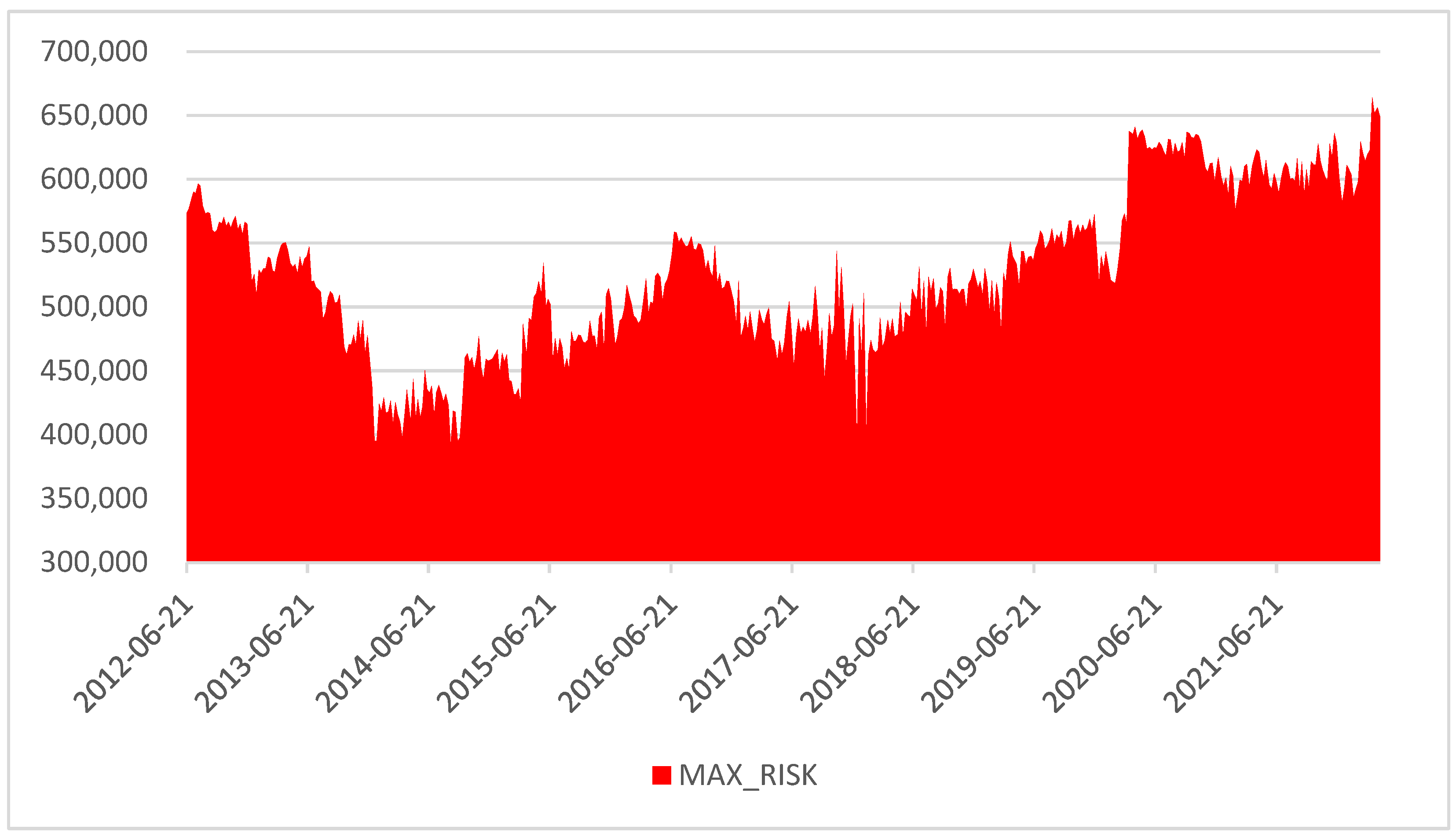
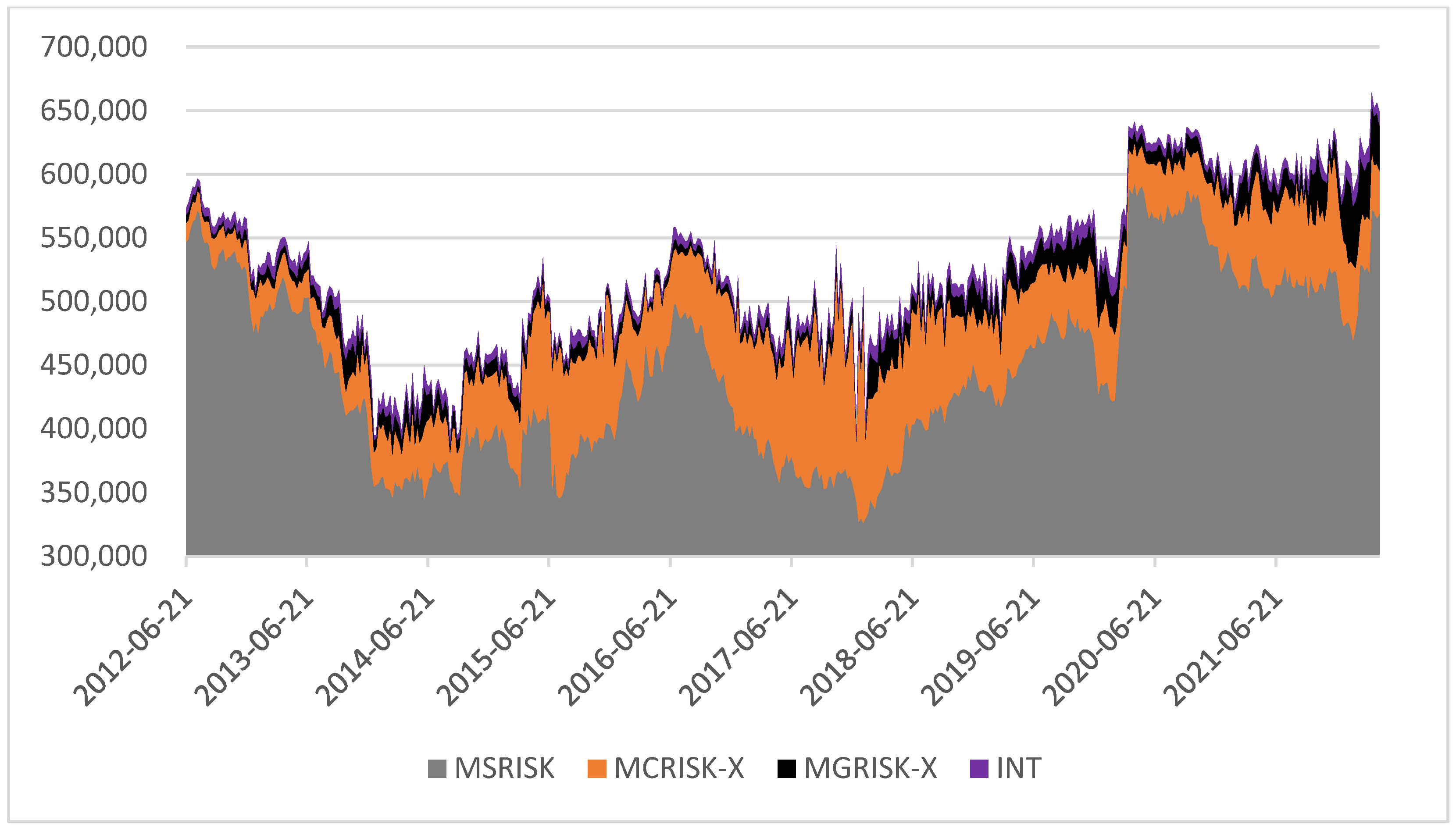
Figure 1 shows aggregate risk MAX_RISK increasing from EUR 573 billion to EUR 649 billion (+13.2%) during the whole period: after bottoming below EUR 400 billion in 2014Q3, it reaches its peak right at the beginning of 2022Q1. Figure 2 decomposes MAX_RISK in MSRISK, MCRISK-X, MGRISK-X, and INT values.

Figure 1.
Aggregate MAX_RISK.
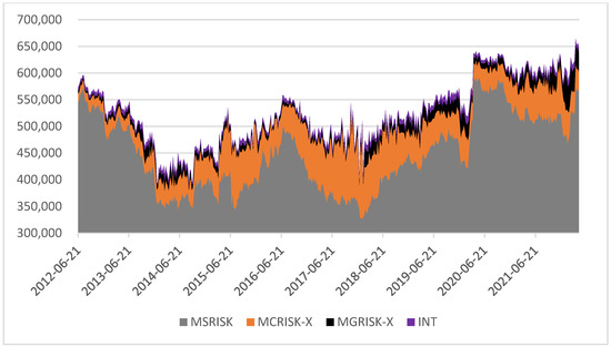
Figure 2.
Aggregate MAX_RISK decomposition.
MSRISK increases from EUR 547 billion to EUR 569 billion (+4.0%), increasing less than MAX_RISK and staying closer to being unchanged, as suggested by the static value in RWA. In line with the findings presented by Gehrig and Iannino (2021), our study reveals that the modest fall in regulatory exposure fails to capture the increase in the aggregate systemic risk, especially considering climate and geopolitical tail risks as measured by MCRISK-X and MGRISK-X.
From July 2011 to April 2022, our proposed climate risk measure MCRISK-X more than doubles, increasing from approximately EUR 15 billion to over EUR 34 billion after surpassing EUR 160 billion following the ratification of the Paris Climate Agreement. On average, MCRISK-X increases MAX_RISK by 13.2% with respect to MSRISK estimates (median hike: 11.5%). As presented in Figure 3, MCRISK-X rose sharply during the 2015 and 2020 energy bear markets25 due to the related surges in transition risk. Conversely, MCRISK-X’s recent fall was likely caused by a temporary reduction in transition risk, likely attributable to the sharp rise in the price of fossil fuels provoked by the breakout of the Russo-Ukrainian war. Given the attention reserved for climate by Eurozone governments and regulators, this situation appears to be transitory: in its 2022 CST exercise, the ECB quantified the potential climate losses for Eurozone financial institutions as approximately EUR 70 billion, of which EUR 53 billion was due to a disorderly transition. It also cautioned that this estimate might significantly understate the extent of the problem. Our aggregate MCRISK-X measure in the first months of 2022 is above EUR 47 billion for a sample of listed banks that represents approximately 70% of the EUROSTOXX sectoral market capitalization. Therefore, we concur with the central bank and conclude that the actual climate risk hanging over the Eurozone financial sector is likely to be somewhat higher than this appraisal.
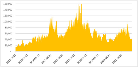
Figure 3.
Tail risk attributable to climate risk MCRISK-X.
A bivariate approach would produce results that strongly diverge from the CST output. Figure 4 compares climate tail risk MCRISK-X with MCRISK and its bivariate equivalent CRISK. MCRISK, represented in our analysis by the event C and the shortfall , that is, when only the climate factor (CFE) breaks the threshold, closely tracks CRISK. Climate risk estimates based on either metric would be, on average, more than nine times those for MCRISK-X26, which also exhibits a markedly different trend. This finding shows the limits of bivariate risk analysis and validates the adoption of a multifactor risk framework in conjunction with the proposed risk attribution methodology.
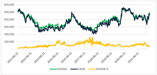
Figure 4.
Multivariate MCRISK vs. bivariate CRISK vs. multivariate MCRISK-X.
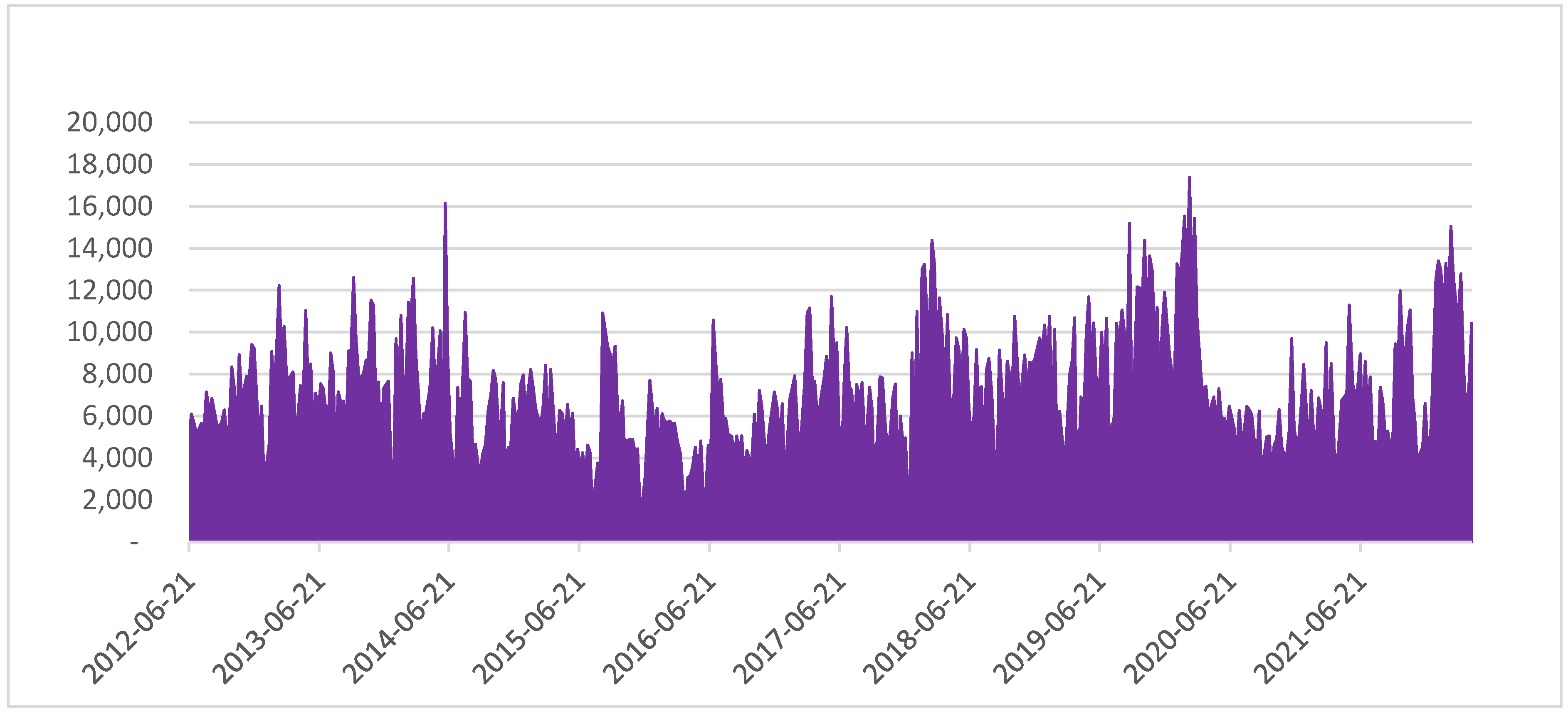
MGRISK-X estimates are presented in Figure 5. By its nature, MGRISK-X is very volatile, influenced by high-impact but low-persistency shocks provoked by events, actions, threats, or news that influence markets for a limited period, with the exception of prolonged wars.
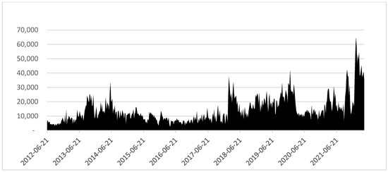
Figure 5.
Tail risk attributable to geopolitical risk MGRISK-X.
Using STATA 16.1 and indicating with (***) a p-value ≤ 0.001, MGRISK-X shows a significative correlation with the Caldara and Iacoviello (2022) GPRD (0.30***) and GPRD Threats (0.46***) indices, developed using Anglo-Saxon news sources. Caldara and Iacoviello publish single-country indices but, to the best of our knowledge, not an aggregate Eurozone geopolitical risk index.
As expected, given the composition of the geopolitical factor GFE, MGRISK-X reacts more noticeably to conflicts27 than to terrorist activity affecting Eurozone member states. From a low of EUR 2 billion in early 2016, MGRISK-X has been propelled to above EUR 64 billion by the breakout of the war in Eastern Europe in early 2022, reaching the highest level recorded during the whole period. On average, MGRISK-X contributes to MAX_RISK 3.2% of MSRISK measures, with a median increase of 2.8%. Worryingly, since 2018, the floor for MGRISK-X seems to have moved higher.
The interaction effect, INT, is presented in Figure 6.

Figure 6.
Tail risk attributable to interaction risk (INT).
Contrary to MCRISK-X and MGRISK-X, this measure of extra risk provoked by the simultaneous occurrence of systemic, climate, and geopolitical crises does not show a particular trend, reaching its peak of approximately EUR 17 billion at the breakout of the pandemic. INT adds, on average, 1.6% of MSRISK estimates to MAX_RISK (median addition: +1.5%).
4.4. Sensitivity Analysis and Robustness Checks
To assess sensitivity, in addition to using the vector (−30%, −35%, and −40%) of threshold values, shortfall estimates were made, employing different rolling 250-day and 500-day time windows. Generally, shorter time frames and higher absolute value thresholds tend to generate larger risks, and with rolling windows, there are some cases of CCC outperforming DCC. However, despite using 75,000 runs per date, the higher the absolute value of the threshold, the greater the number of instances that require data interpolation for both 250- and 500-day rolling windows to estimate certain risk measures continuously. Therefore, the results presented were obtained using the expanding method.
Both the MAX_RISK and MSRISK estimates tend to grow with the absolute value of the threshold, whereas the dispersion tends to contract (Table 2), as shown by the ratio of the respective measures calculated with different thresholds.
Table 2.
Sensitivity analysis—MAX_RISK and MSRISK threshold ratios.
In Table 2, Table 3, Table 4 and Table 5, Ratio_x/y indicates the ratio of the estimates computed with threshold x% and threshold y%, respectively.
Even with thresh set at −40%, only one date (25 January, 2013) required data interpolation to obtain MSRISK, proving the reliability of the expanding (recursive) window method.
In terms of stability, the MCRISK-X estimates are not very sensitive to changes to the absolute value of the threshold, which tends to increase dispersion rather than affect the magnitude of the climate risk estimate, as reported in Table 3.
Table 3.
Sensitivity analysis—MCRISK-X threshold ratios.
Table 3.
Sensitivity analysis—MCRISK-X threshold ratios.
| Ratio_35/30 | Ratio_40/35 | Ratio_40/30 | |
|---|---|---|---|
| Mean: | 97.0% | 93.3% | 90.5% |
| StdDev: | 14.8% | 19.9% | 23.2% |
| Min: | 38.3% | 18.5% | 17.1% |
| Max: | 164.0% | 205.9% | 195.7% |
As mentioned, we also calculated MCRISK-X using rolling windows: in both instances, the resulting metric values show wider swings, indicating the transition risk spikes that occurred in 2015 and 2020 very well. In both instances, the surges were followed by a sharp decline.
As presented in Table 4, in terms of MGRISK-X, the choice of the threshold appears to affect the dispersion more than its value:
Table 4.
Sensitivity analysis—MGRISK-X threshold ratios.
Table 4.
Sensitivity analysis—MGRISK-X threshold ratios.
| Ratio_35/30 | Ratio_40/35 | Ratio_40/30 | |
|---|---|---|---|
| Mean: | 100.8% | 100.3% | 100.7% |
| StdDev: | 25.0% | 33.9% | 39.3% |
| Min: | 23.0% | 0.0% | 0.0% |
| Max: | 281.8% | 330.4% | 401.0% |
Using 250-day and 500-day rolling windows, MGRISK-X shows prolonged periods of zero or near-zero geopolitical risk, followed by spikes before the Crimean crisis in 2014 and the breakout of the COVID-19 pandemic and the Russo-Ukrainian war. The interaction estimates are not very sensitive to threshold changes, as shown in Table 5.
Table 5.
Sensitivity analysis—INT threshold ratios.
Table 5.
Sensitivity analysis—INT threshold ratios.
| Ratio_35/30 | Ratio_40/35 | Ratio_40/30 | |
|---|---|---|---|
| Mean: | 94.7% | 93.9% | 90.5% |
| StdDev: | 20.4% | 28.8% | 37.2% |
| Min: | 0.0% | 0.0% | 0.0% |
| Max: | 186.8% | 233.8% | 253.0% |
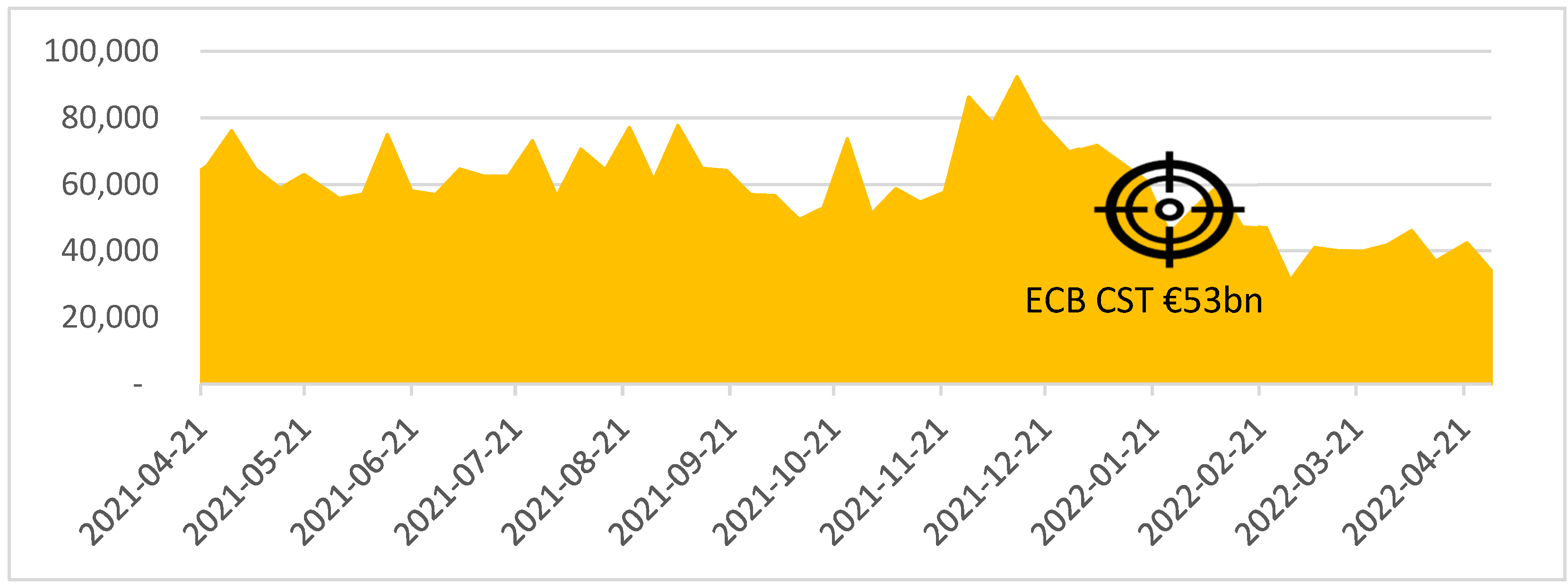
The robustness of our results was confirmed by two important checks. In January 2022, MCRISK-X, which is our measure of transition risk for 70% of the Eurozone banking sector, was EUR 47 bn: as shown in Figure 7, this value is compatible with that of EUR 53 bn estimated by the ECB Climate Stress Test for all the lenders in the single-currency area. The ECB CST arrived at this result by using a granular analysis based on banks’ loan portfolios, and it is considered by the central bank as a floor for climate risk. We concur with this assessment.

Figure 7.
Robustness check—climate tail risk MCRISK-X vs. ECB CST.
To the best of our knowledge, there are no other quantitative assessments of geopolitical risk for Eurozone banks. Hence, we checked MGRISK-X correlations with the indices developed by Caldara and Iacoviello (2022) across the entire period. Lacking a specific Eurozone geopolitical risk gauge, we used the GPRD and the Threats time series, constructed using Anglo-Saxon news sources. In both cases, the correlation was positive and significant, as shown in Table 6.
Table 6.
Robustness check—geopolitical tail risk MGRISK-X correlation with GPRD and Threats. (***) p-value ≤ 0.001.
5. Conclusions
We have developed a multifactor framework that allows for tail risk assessment and attribution. This approach manages to identify a dominant risk factor, if present, and uses it as a reference to quantify and allocate tail risk to other concurrent sources when events of a different nature occur at once.
The application of this methodology to a sample of large Eurozone lenders produced several interesting findings that are robust to changes in factor thresholds:
- (1)
- Systemic risk is identified as the dominant risk factor for Eurozone banks. Furthermore, our analysis indicates that, on average, current systemic risk estimates obtained using a bivariate approach underestimate potential aggregate losses by EUR 77.1 billion (median: EUR 75.6 billion), or 18.1% (median: 17.1%). This undershooting is caused by the effects of the interaction between the different types of risk and can be captured only via a multivariate analysis.
- (2)
- The proposed climate tail risk attribution model produces a result that is comparable with the ECB climate stress test’s appraisal, even though their EUR 53 billion transition risk assessment is likely to be moderately optimistic (i.e., lower than the actual risk). Conversely, bivariate approaches overestimate climate risk by almost one order of magnitude. This overshooting is provoked by the overlapping of capital shortfall estimates that fails to consider the dominant risk, that is, systemic risk, as the major source of potential negative equity comprising the losses of isolated events of different natures. However, climate risk does constitute a dangerous source or tail risk if combined with systemic and geopolitical issues. Its mean addition to systemic risk is, on average, EUR 55.7 billion (median: EUR 51.6 billion), representing 10.8% of the maximum potential aggregate shortfall (median: 9.9%). It can account for up to 32.1% of maximum combined losses during energy bear markets. In the period considered, despite its late drop, climate tail risk more than doubled. This methodology is ineffective in measuring physical risk, which, due to its nature, requires a granular geospatial database that cannot be effectively replaced by using only market data. The ECB CST has quantified physical risk as one third of transition risk, or a quarter of total climate risk.
- (3)
- Geopolitical risk adds EUR 14.3 billion (median: EUR 11.9 billion) to mean systemic risk, representing, on average, 2.7% (median: 2.3%) of the aggregate maximum risk if combined with systemic and climate events. During the dramatic period leading to the breakout of the war in Ukraine, tail risk linked to the geopolitical factor surged to EUR 64.7 billion, or 10.6% of maximum aggregate losses, thereby reaching the maximum incidence across the entire period analyzed. Further refinements in the geopolitical factor (GFE) would certainly improve the accuracy and timeliness of the results, which are significantly correlated with Caldara and Iacoviello’s (2022) Threats index.
- (4)
- Interaction risk is a byproduct of the simultaneous occurrence of multiple crises that can be measured only within this type of multivariate framework. It does not show any specific trend and represents, on average, 1.4% (median: 1.3%) of total risk. However, it never drops to zero and can reach 3.6% of combined aggregate losses, thereby indicating latent potential excess shortfall.
- (5)
- Our results are in line with those acquired by Gehrig and Iannino (2021) in suggesting that the relative stability of risk-weighted exposure reported by Eurozone banks does not reflect the actual trajectory of their aggregate risk, which was higher in 2022 than in 2011.
- (6)
- These findings could be used to develop portfolio construction techniques robust to multiple shocks. Lin et al. (2023) have introduced a suite of metrics based on bivariate designed to identify portfolios of banks able to overperform during systemic crises, whereas MCRISK-X and MGRISK_X could be utilized to perform sectoral stock selection to minimize the impact of climate and geopolitical shocks on portfolio returns. We are currently in the process of investigating this subject further with our forthcoming “Identifying green banks” paper.
This approach can be used to explore the effects of simultaneous, manifold risk occurrences on Eurozone capital buffers. In these instances, traditional bivariate risk measures significantly underestimate aggregate shortfall: increased instability could lead regulators to enact drastic measures, similar to the mandatory cancellation of approved bank dividends in the spring of 2020. This decision had the benefit of immediately improving Eurozone banks’ equity base but also caused relevant collateral damage, especially in the derivatives market. The proposed multifactor risk assessment framework can serve as an early-warning tool, alerting markets that severe actions might be forthcoming. Moreover, it can quantify climate and geopolitical tail risk, offering important hindsight on how to adapt regulatory frameworks to rapidly mutating risk factors. As shown by Gouriéroux et al. (2022), the identification of optimal capital requirements becomes extremely difficult when long-term challenges, such as the transition to a carbon neutral economy, must be reconciled with short-term micro-prudential considerations. In a world with rising risks of different natures, regulation needs to ensure systemic integrity while preserving Eurozone banks’ capability to produce earnings and strengthening their capital bases because a well-supervised and successful banking sector is necessary to achieve long-term financial stability. Hopefully, the methodology proposed in this work will contribute to achieving such a goal.
Author Contributions
Conceptualization, M.C.R. and G.M.M.; Methodology, M.C.R. and G.M.M.; Software, G.M.M.; Validation, G.B.; Formal analysis, G.M.M.; Investigation, G.M.M.; Resources, G.M.M.; Data curation, G.M.M.; Writing—original draft, G.M.M.; Writing—review & editing, G.B.; Supervision, M.C.R. All authors have read and agreed to the published version of the manuscript.
Funding
This research did not receive any specific grant from funding agencies in the public, commercial, or not-for-profit sectors.
Data Availability Statement
Data available at https://sl.univpm.it/CX50626, accessed on 12 July 2022.
Conflicts of Interest
The authors declare no conflict of interest.
Appendix A
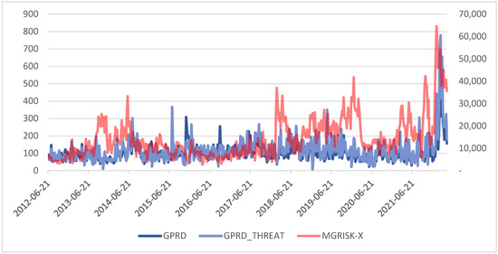
Figure A1.
GPRD, THREATS indices, and MGRISK-X (right scale). Data downloaded from https://www.matteoiacoviello.com/gpr.htm accessed on 3 November 2022.
Figure A1.
GPRD, THREATS indices, and MGRISK-X (right scale). Data downloaded from https://www.matteoiacoviello.com/gpr.htm accessed on 3 November 2022.
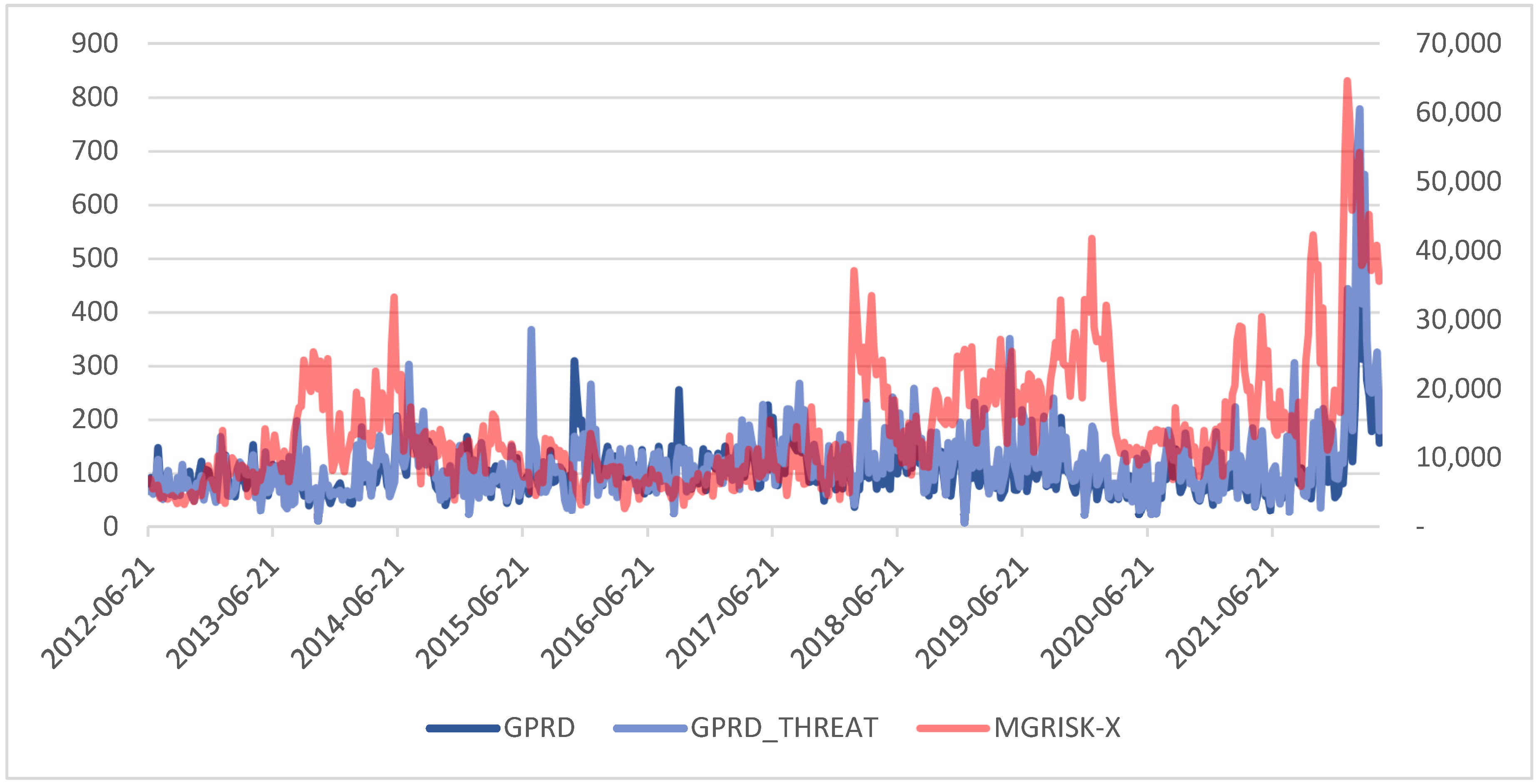
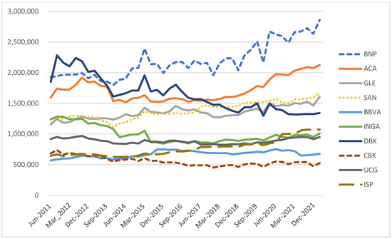
Figure A2.
Evolution of Total Assets (TA) for the selected sample.
Figure A2.
Evolution of Total Assets (TA) for the selected sample.
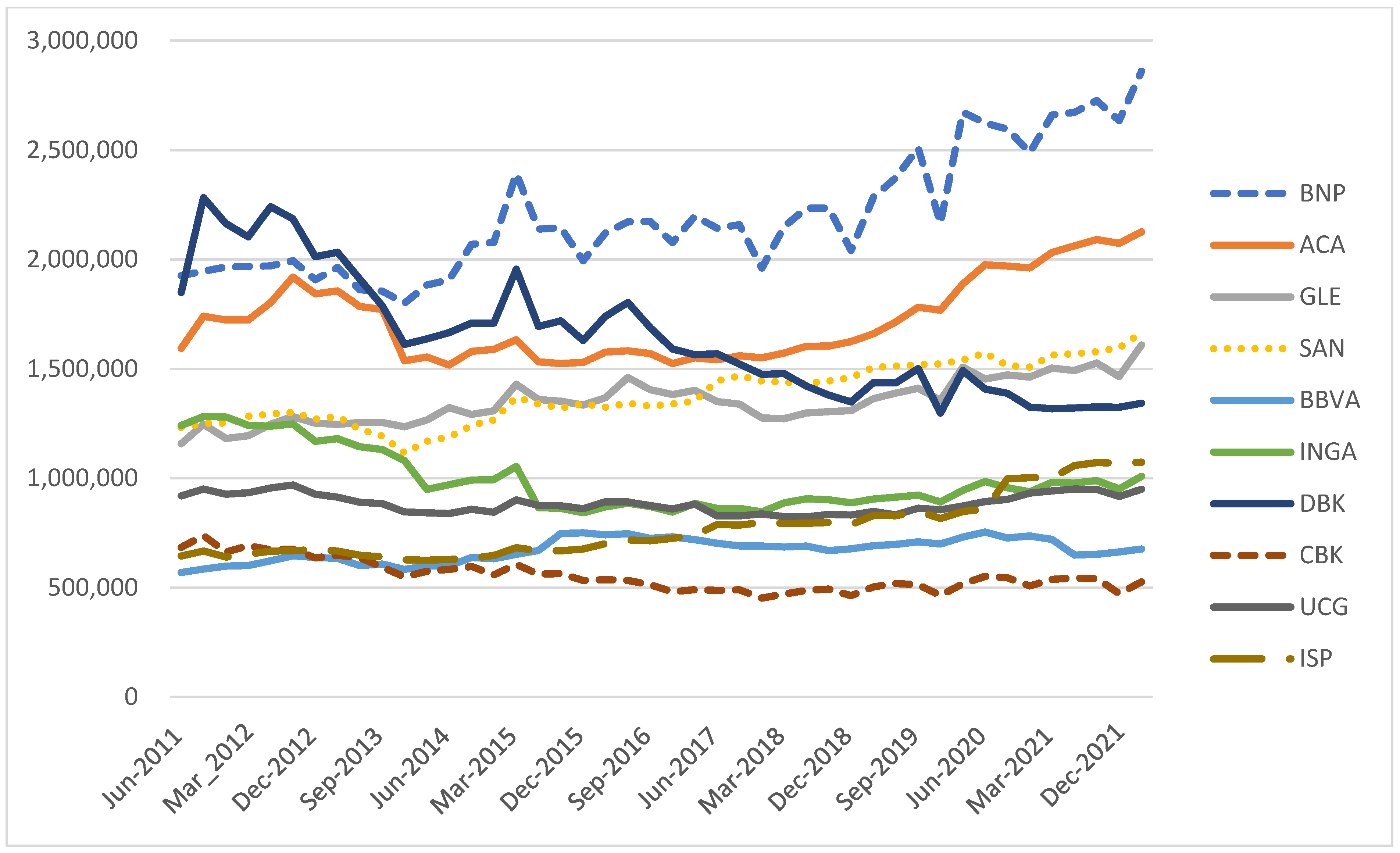
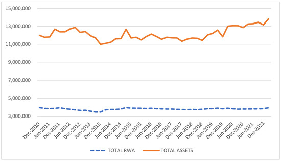
Figure A3.
Evolution of aggregate Total Assets and aggregate Risk-Weighted assets for the sample.
Figure A3.
Evolution of aggregate Total Assets and aggregate Risk-Weighted assets for the sample.
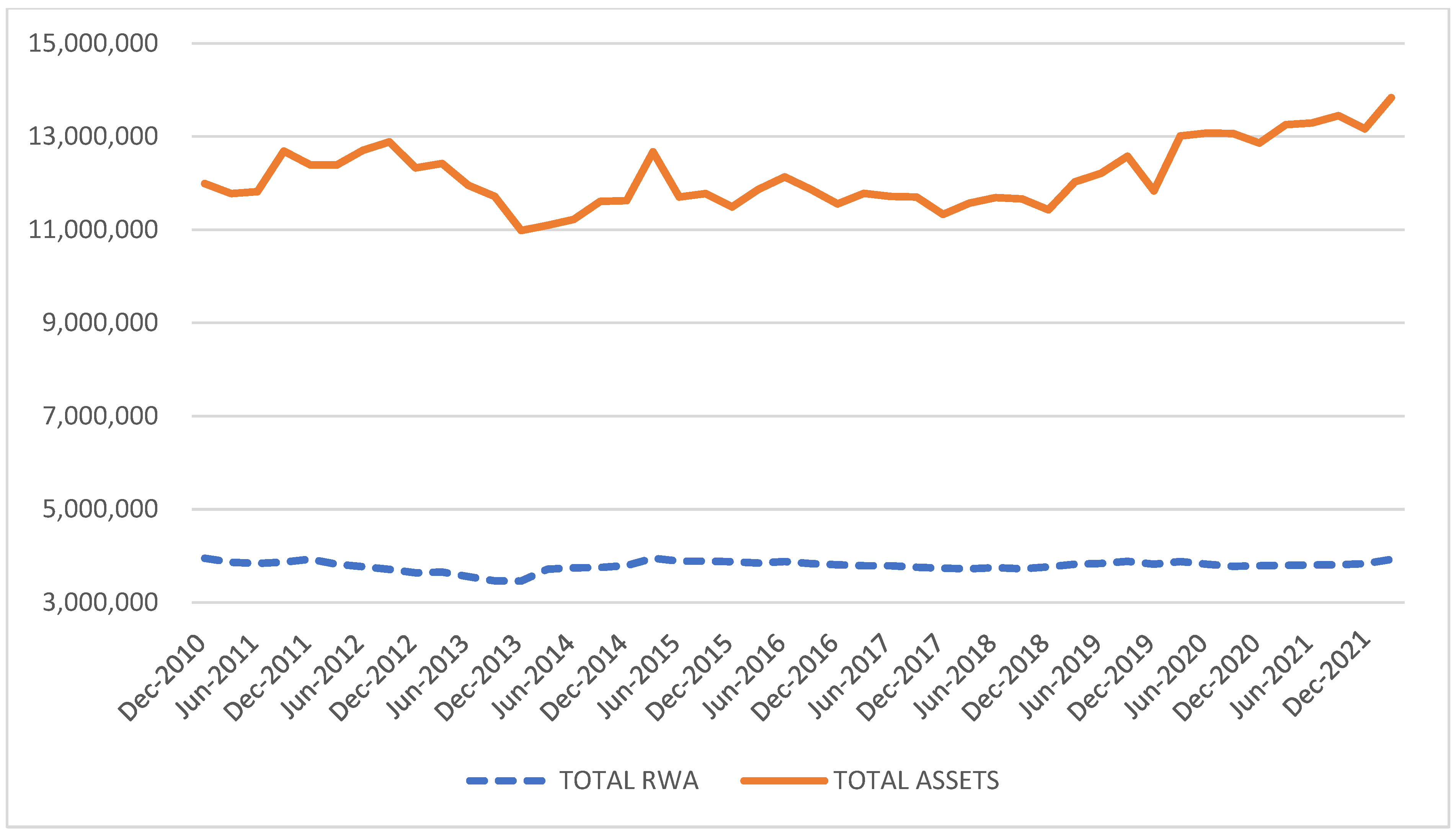
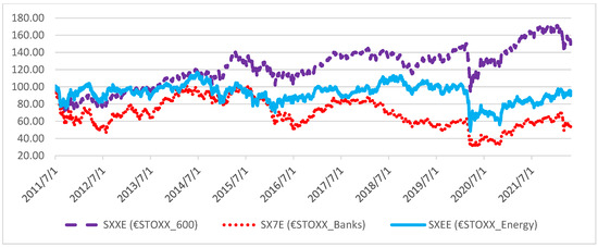
Figure A4.
SXXE vs. SX7E vs. SXEE, Q3/2021–Q2/2022.
Figure A4.
SXXE vs. SX7E vs. SXEE, Q3/2021–Q2/2022.
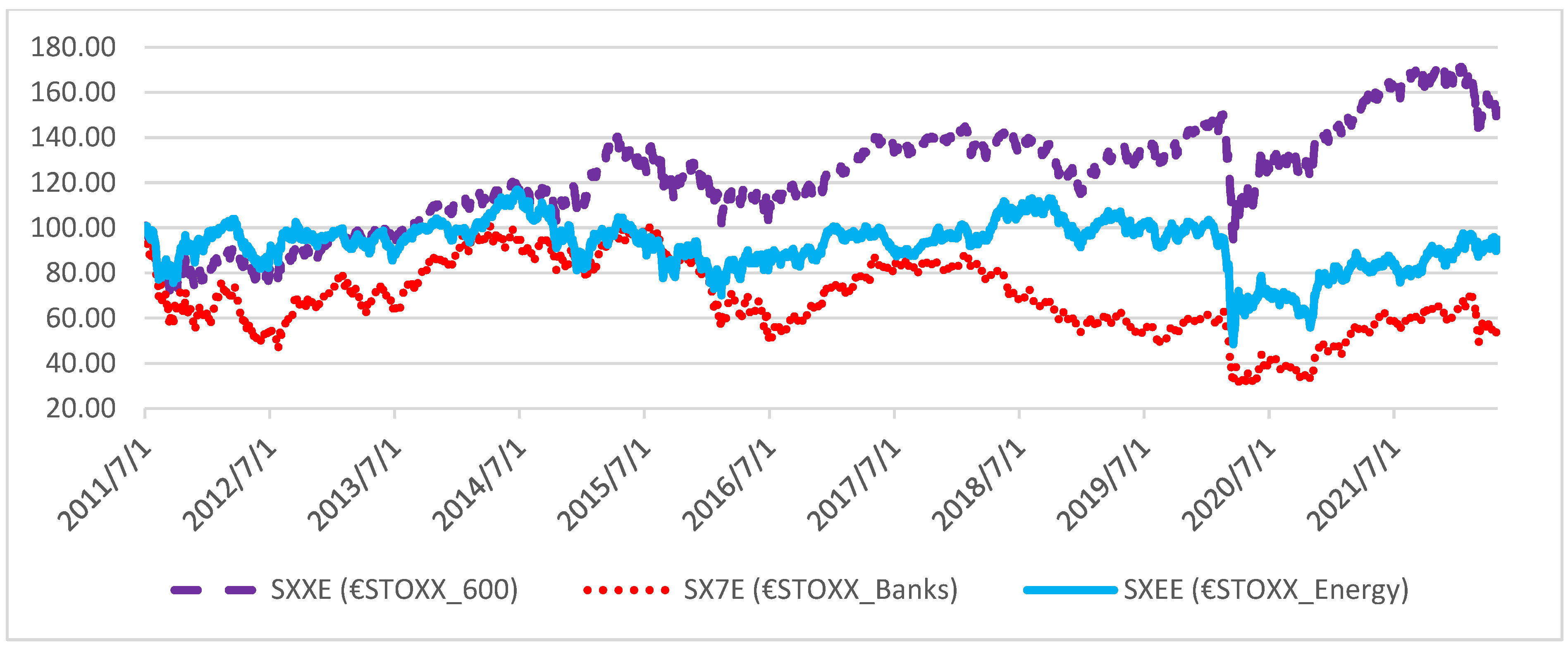
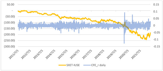
Figure A5.
CFE (SXET-IUSE) and daily dispersion (right scale).
Figure A5.
CFE (SXET-IUSE) and daily dispersion (right scale).
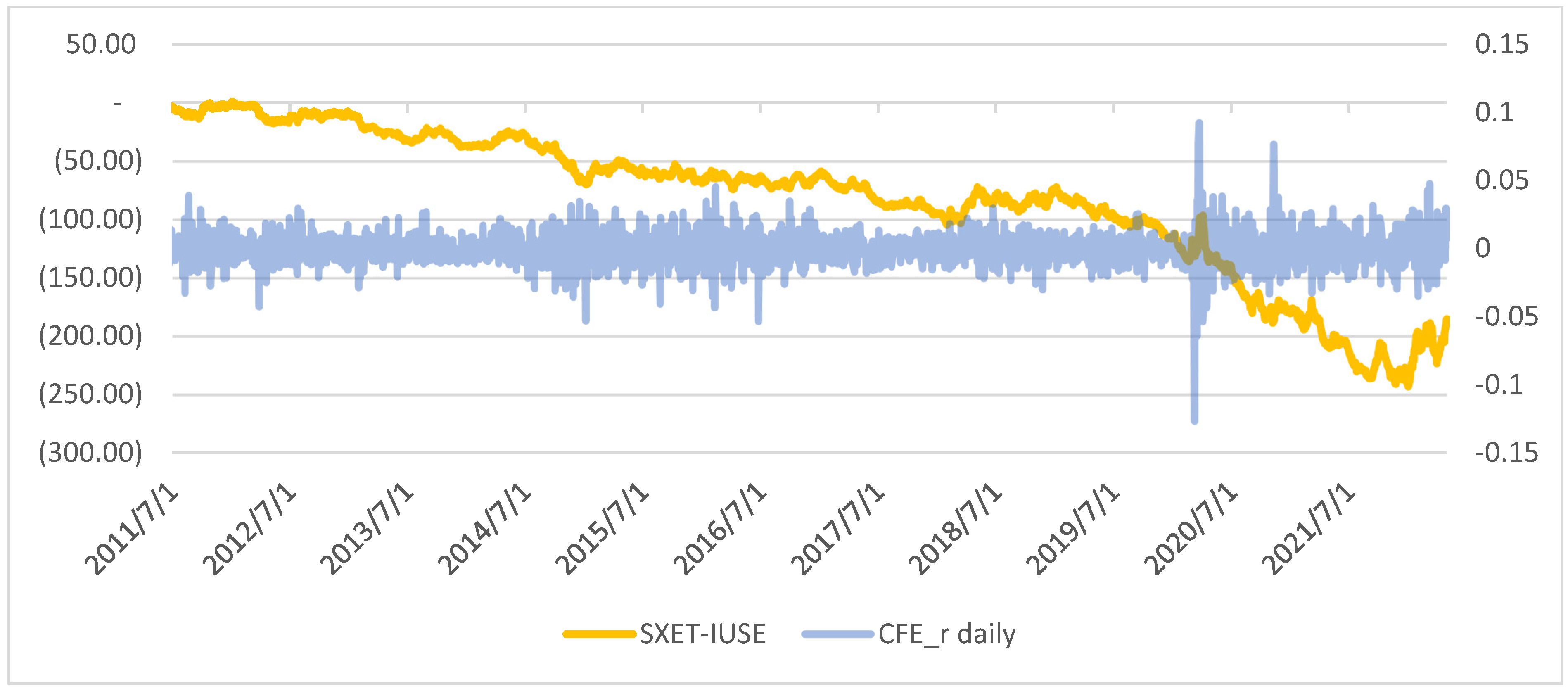

Figure A6.
GFE (0.5 SXRARO + 0.5 PHAU—IUSE) and daily dispersion (right scale).
Figure A6.
GFE (0.5 SXRARO + 0.5 PHAU—IUSE) and daily dispersion (right scale).
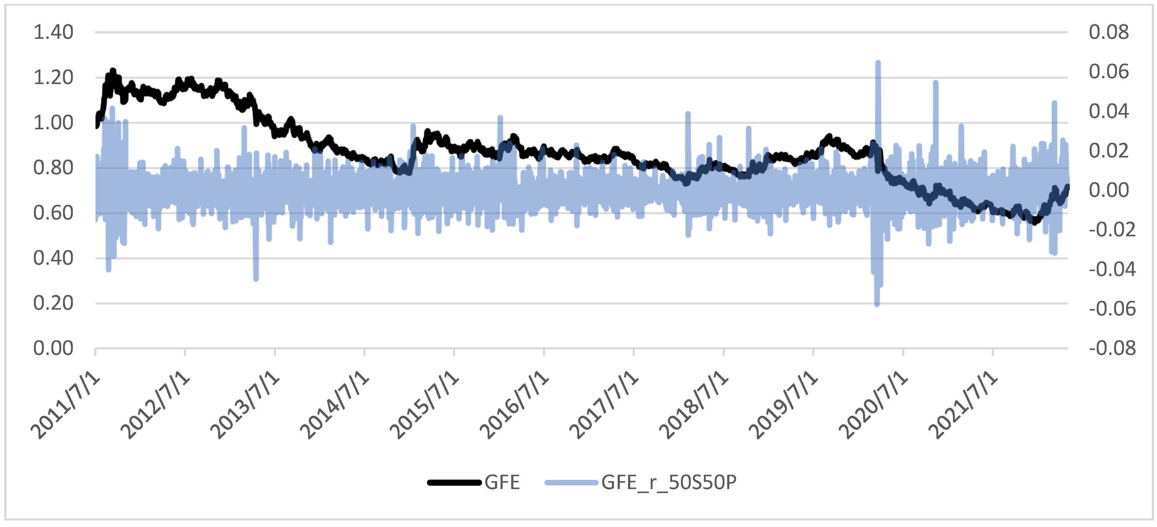
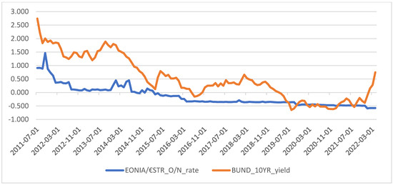
Figure A7.
Eurozone interest rates, 2011Q3–2022Q1A2. Eurozone interest rates, 2011Q3–2022Q1.
Figure A7.
Eurozone interest rates, 2011Q3–2022Q1A2. Eurozone interest rates, 2011Q3–2022Q1.
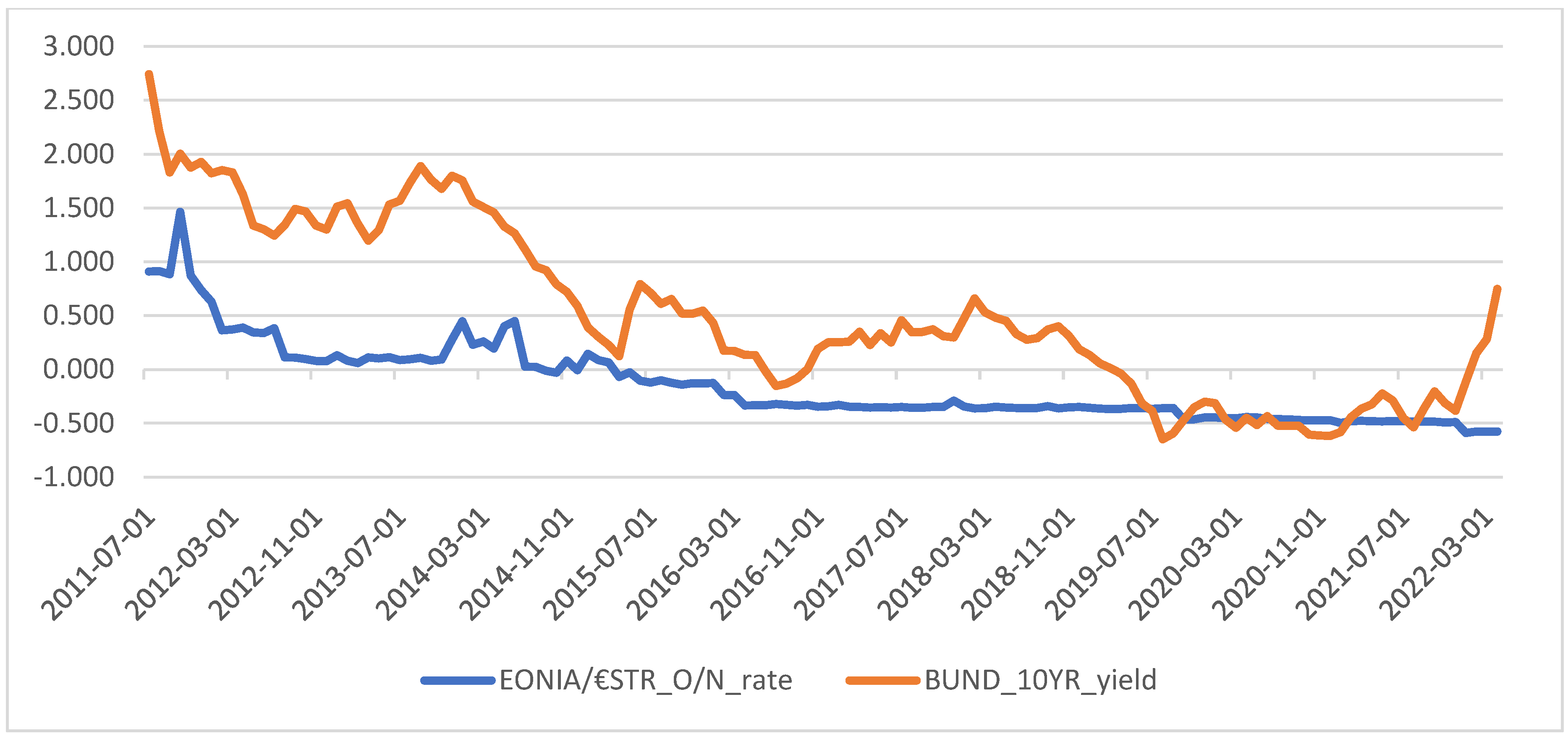
Table A1.
Tse test conducted on the entire sample (OxMetrics 8.2).
Table A1.
Tse test conducted on the entire sample (OxMetrics 8.2).
| LM Test for Constant Correlation of Tse (2000) |
| LMC: 38.0318 [0.0000000] |
| p-value in brackets. LMC~X2(N*(N − 1)/2)) under H0: CCC model, with N = #series |
Table A2.
Engle–Sheppard test for dynamic correlation (OxMetrics 8.2).
Table A2.
Engle–Sheppard test for dynamic correlation (OxMetrics 8.2).
| E-S Test(5) = 70.3061 [0.0000000] |
| E-S Test(10) = 116.544 [0.0000000] |
| p-values in brackets. E-S Test(j)~X2(j + 1) under H0: CCC model |
Table A3.
Full-sample CCC-DCC comparison (OxMetrics 8.2).
Table A3.
Full-sample CCC-DCC comparison (OxMetrics 8.2).
| Model | T | p | Log-Likelihood | SC | HQ | AIC |
|---|---|---|---|---|---|---|
| MG@RCH(1) | 2735 | 3 | 26970.570 | −19.714 | −19.718 | −19.720 |
| MG@RCH(2) | 2735 | 5 | 27078.285 | −19.787< | −19.794< | −19.798< |
Table A4.
Excluded dates (MM/DD/YYYY).
Table A4.
Excluded dates (MM/DD/YYYY).
| 8/15/2011, 5/1/2012, 8/15/2012, 12/24/2012, 12/31/2012, 5/1/2013, 8/15/2013, 12/24/2013, 12/26/2013, 12/31/2013, 5/1/2014, 8/15/2014, 10/3/2014, 12/24/2014, 12/26/2014, 12/31/2014, 5/1/2015, 5/25/2015, 12/24/2015, 12/31/2015, 5/16/2016, 8/15/2016, 10/3/2016, 12/26/2016, 5/1/2017, 6/5/2017, 8/15/2017, 10/3/2017, 10/31/2017, 5/1/2018, 5/21/2018, 8/15/2018, 10/3/2018, 12/24/2018, 12/31/2018, 5/1/2019, 6/10/2019, 8/15/2019, 10/3/2019, 12/24/2019, 12/31/2019, 5/1/2020, 6/1/2020, 12/24/2020, 12/31/2020, 5/24/2021, 12/24/2021, 12/31/2021. |
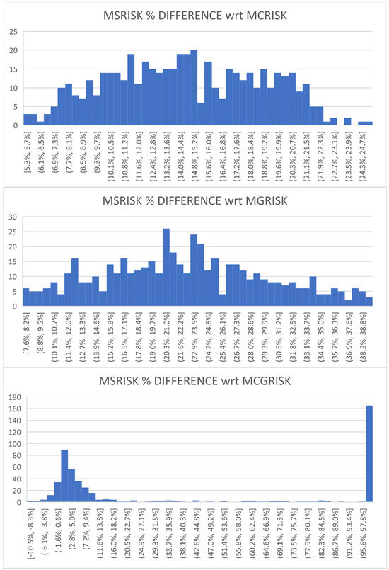
Figure A8.
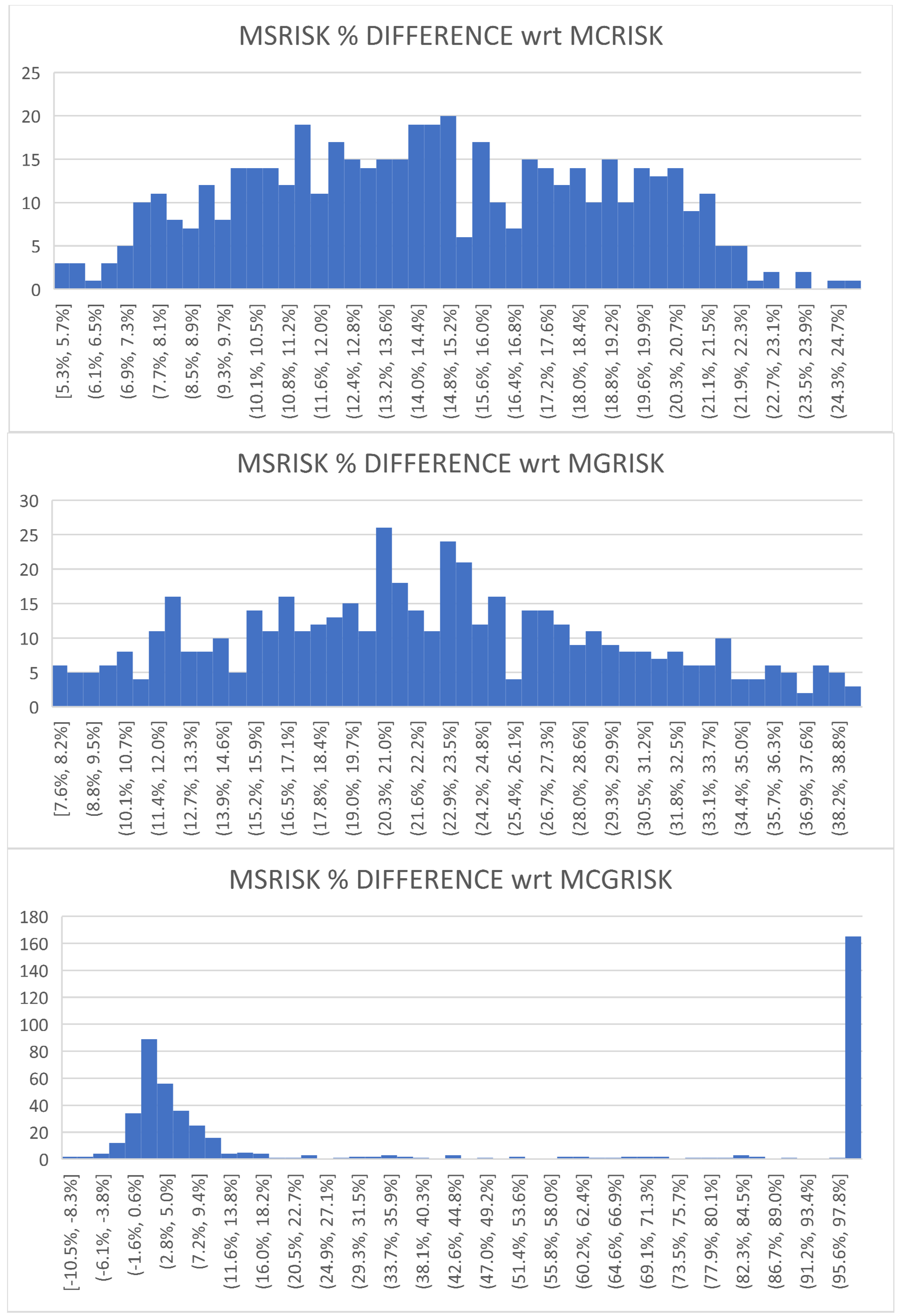
MSRISKt percentage differences with respect to MCRISKt, MGRISKt, and MCGRISKt.
Figure A8.
MSRISKt percentage differences with respect to MCRISKt, MGRISKt, and MCGRISKt.
Notes
| 1 | The work by Battiston et al. (2017) laid the basis for including the evolution of carbon emissions and temperatures in a comprehensive climate stress-test effort, whereas Roncoroni et al. (2021) proposed combining the stress test approach with network evaluation analysis to investigate the higher-round effects of a climate crisis on the financial sector. |
| 2 | European Central Bank (ECB-ESBR) (2022), “2022 climate risk stress test”, July. |
| 3 | For an alternative, network-based approach, see Roncoroni et al. (2021). |
| 4 | See Caldara and Iacoviello (2022), “Measuring Geopolitical Risk”, American Economic Review, April, 112(4), pp. 1194–1225, https://www.matteoiacoviello.com/gpr.htm accessed on 3 November 2022. |
| 5 | See, for example, https://vlab.stern.nyu.edu/georisk (accessed on 3 November 2022) published by the NYU. |
| 6 | For example, the Blackrock Investment Institute Geo-political risk dashboard. |
| 7 | For a comprehensive discussion on this matter, see Admati and Hellwig (2013). |
| 8 | During times of crisis, the total amount of bank debt tends to have small absolute fluctuations, even if its composition might vary: a reduction in deposits might be compensated by an increase in other types of funding, often provided by central banks. The no bail-in assumption implies that bank bonds are set to be reimbursed without haircuts. |
| 9 | A geopolitical event causing flight-to-quality flows is likely to produce an increase, and not a fall, in GFE. |
| 10 | See Section 4.3 for the details. |
| 11 | Under the constraint φ + λ + γ/2 < 1 for a Gaussian distribution. |
| 12 | See Threshold Arch Models and Asymmetries in Volatility by Rabemananjara and Zakoian (1993). |
| 13 | See index provider Qontigo—https://www.stoxx.com/index-details?symbol=sxxe (accessed on 12 July 2022). |
| 14 | During the period considered, the S&P500 index represented more than 60% of the MSCI World Index. |
| 15 | There are valid alternatives to IUSE, such as Lyxor’s SP5H/SPXH, but not with a price history encompassing the entire period considered. |
| 16 | IUSE was launched in the fall of 2010; since then, it has tracked the dollar-denominated SPX very well: in the period considered, the iShare ETF cumulated daily and yearly log returns show a 99.9% correlation with the corresponding SPX USD return statistics. Given the currency hedge and the fact that the price of IUSE is arbitraged until the close of European business, it is our opinion that the characteristics of this ETF eliminate the need to account for lagged returns in this type of analysis. |
| 17 | See the Appendix A, Table A4, for a full list of excluded dates. |
| 18 | A preliminary analysis on the full sample was conducted using the Tse (2000) and the Engle and Sheppard (2001) tests. See Appendix A Table A1 and Table A2 for details. |
| 19 | OxMetrics 8.2 and Matlab R2021b, integrated with the MFE Toolbox developed by K. Sheppard and the Parallel Computing module. |
| 20 | Jung et al. (2021) uses a 50% climate factor drop in 6 months as a crisis threshold. Considering the distributions of realized returns in our sample, we deem such a steep fall unrealistic for our specific purpose. |
| 21 | Sectoral stock selection robust to climate risk is discussed in our forthcoming study, “Identifying green banks”. |
| 22 | On their VLAB website, the NYU publishes bivariate CRISK estimates. (see https://vlab.stern.nyu.edu/climate), accessed on 13 June 2022. |
| 23 | In the cases when does exceed , we found that is, on average, larger than by 2.8%. |
| 24 | As explained in Section 4.2, the observation period spans from the beginning of July 2011 to the end of April 2022, using a 5-day interval between measurements, amounting to a total of 498 dates. The threshold thresh was set at −30%, whereas the Monte Carlo simulation was conducted with 75,000 runs over a 63-day period (3 months) per date per bank. |
| 25 | In both instances, Brent crude prices dropped more than 50%. |
| 26 | These findings are in line with the NYU V-Lab output: for the selected sample, the C event generated a multivariate MCRISK estimate on 29 April, 2022, equal to EUR 490 billion, which can be compared with a bivariate V-LAB measurement of USD 469 billion: considering the prevailing FX rate at the time of EUR/USD = 1.05, this equates to a EUR 446 billion bivariate CRISK, or 91.1% of our MCRISK estimate produced in a multivariate context using a different climate factor. Site accessed on 13 June 2022. |
| 27 | Such as the annexation of Crimea in 2014, the fall of the ISIS Caliphate in late 2017–2018, and the North Korean crisis in 2018–2019. |
References
- Acharya, Viral V., Lasse H. Pedersen, Thomas Philippon, and Matthew Richardson. 2017. Measuring systemic risk. The Review of Financial Studies 30: 2–47. [Google Scholar] [CrossRef]
- Admati, Anat, and Martin Hellwig. 2013. The Bankers’ New Clothes: What’s Wrong with Banking and What to Do about It, 9th ed. Princeton and Oxford: Princeton University Press. ISBN 978-0-691-16238-6. [Google Scholar]
- Adrian, Thobias, and Markus K. Brunnermeier. 2016. CoVaR. American Economic Review 106: 1705–41. [Google Scholar] [CrossRef]
- Allen, Franklin, and Elena Carletti. 2013. What Is Systemic Risk? Journal of Money, Credit and Banking 45: 121–27. [Google Scholar] [CrossRef]
- Battiston, Stefano, Antoine Mandel, Irene Monasterolo, Franziska Schütze, and Gabriele Visentin. 2017. A climate stress test of the financial system. Nature Climate Change 7: 283–88. [Google Scholar] [CrossRef]
- Battiston, Stefano, Domenico Delli Gatti, Mauro Gallegati, Bruce Greenwald, and Joseph E. Stiglitz. 2012. Liaisons dangereuses: Increasing connectivity, risk sharing, and systemic risk. Journal of Economic Dynamics and Control 36: 1121–41. [Google Scholar] [CrossRef]
- Bollerslev, Tim. 1990. Modelling the Coherence in Short-Run Nominal Exchange Rates: A Multivariate Generalized Arch Model. The Review of Economics and Statistics 72: 498–505. [Google Scholar] [CrossRef]
- Brownlees, Christian, and Robert F. Engle. 2017. SRISK: A conditional capital shortfall measure of systemic risk. The Review of Financial Studies 30: 48–79. [Google Scholar] [CrossRef]
- Caldara, Dario, and Matteo Iacoviello. 2022. Measuring Geopolitical Risk. American Economic Review 112: 1194–225. [Google Scholar] [CrossRef]
- Engle, Robert F. 2002. Dynamic Conditional Correlation: A Simple Class of Multivariate Generalized Autoregressive Conditional Heteroskedasticity Models. Journal of Business & Economic Statistics 20: 339–50. [Google Scholar] [CrossRef]
- Engle, Robert F. 2009. Anticipating Correlations. Princeton: Princeton University Press. ISBN 9780691116419. [Google Scholar]
- Engle, Robert F. 2016. Dynamic Conditional Beta. Journal of Financial Econometrics 14: 643–67. [Google Scholar] [CrossRef]
- Engle, Robert F., and Kevin Sheppard. 2001. Theoretical and Empirical Properties of Dynamic Conditional Correlation Multivariate GARCH. No 8554, NBER Working Papers, National Bureau of Economic Research, Inc. Available online: https://EconPapers.repec.org/RePEc:nbr:nberwo:8554 (accessed on 11 March 2022).
- Engle, Robert F., Eric Jondeau, and Michael Rockinger. 2015. Systemic Risk in Europe. Review of Finance 19: 145–90. [Google Scholar] [CrossRef]
- European Central Bank (ECB-ESRB). 2021. Climate-Related Risk and Financial Stability. July. Available online: https://www.ecb.europa.eu/press/pr/date/2021/html/ecb.pr210701~8fe34bbe8e.en.html (accessed on 4 April 2022).
- European Central Bank (ECB-ESBR). 2022. 2022 Climate Risk Stress Test. July. Available online: https://www.ecb.europa.eu/press/pr/date/2022/html/ecb.pr220726~491ecd89cb.en.html (accessed on 31 August 2022).
- Gehrig, Thomas, and Maria C. Iannino. 2021. Did the Basel Process of capital regulation enhance the resiliency of European banks? Journal of Financial Stability 55: 100904. [Google Scholar] [CrossRef]
- Glosten, Lawrence, Ravi Jagannathan, and David E. Runkle. 1993. On the relation between the expected value and the volatility of the excess returns on stocks. The Journal of Finance 48: 1779–801. [Google Scholar] [CrossRef]
- Gouriéroux, Christian, Alain Monfort, and Jean-Paul Renne. 2022. Required Capital for Long-Run Risks. Journal of Economic Dynamics and Control 144: 104502. [Google Scholar] [CrossRef]
- Hull, John C. 2023. Risk Management and Financial Institutions, 6th ed. Hoboken: Wiley. ISBN 978-1-119-93249-9. [Google Scholar]
- Jung, Hyeyoon, Robert F. Engle, and Richard Berner. 2021. CRISK: Measuring the Climate Risk Exposure of the Financial System. FRB of New York Staff Report No. 977, Rev. March 2023. Previous title: “Climate Stress Testing”. Available online: https://ssrn.com/abstract=3931516.html (accessed on 4 April 2022).
- Lin, Weidong, Jose Olmo, and Abderrahim Taamouti. 2023. Portfolio Selection under Systemic Risk. Journal of Money, Credit and Banking. early view. [Google Scholar] [CrossRef]
- Rabemananjara, Roger, and Jean-Michel Zakoian. 1993. Threshold Arch Models and Asymmetries in Volatility. Journal of Applied Econometrics 8: 31–49. [Google Scholar]
- Roncoroni, Alan, Stefano Battiston, Luiso O. L. Escobar-Farfán, and Serafin Martinez-Jaramillo. 2021. Climate risk and financial stability in the network of banks and investment funds. Journal of Financial Stability 54: 100870. [Google Scholar] [CrossRef]
- Tse, Yiu Kuen. 2000. A test for constant correlations in a multivariate GARCH model. Journal of Econometrics 98: 107–27. [Google Scholar] [CrossRef]
- Zhang, Xingmin, Qiang Fu, Liping Lu, Qingyu Wang, and Shuai Zhang. 2021. Bank liquidity creation, network contagion and systemic risk: Evidence from Chinese listed banks. Journal of Financial Stability 53: 100844. [Google Scholar] [CrossRef]


Disclaimer/Publisher’s Note: The statements, opinions and data contained in all publications are solely those of the individual author(s) and contributor(s) and not of MDPI and/or the editor(s). MDPI and/or the editor(s) disclaim responsibility for any injury to people or property resulting from any ideas, methods, instructions or products referred to in the content. |
© 2023 by the authors. Licensee MDPI, Basel, Switzerland. This article is an open access article distributed under the terms and conditions of the Creative Commons Attribution (CC BY) license (https://creativecommons.org/licenses/by/4.0/).