Abstract
In a recent paper “Stochastic Chain-Ladder Reserving with Modeled General Inflation”, the effects of modeled general inflation on non-life claims reserving were studied using, along with the so called “market approach”, a stochastic two-factor market model, characterized by deterministic expected inflation. In the present paper, we repeat the same study, again with the market approach, using a three-factor market model which extends the two-factor model by including stochastic expected inflation. After detailing the theoretical model and estimating the relevant parameters on the same market data used in “Stochastic Chain-Ladder Reserving with Modeled General Inflation”, we repeat the application to claims reserving presented in that paper and compare the results obtained with the two models. With these data, it is found that the inclusion of stochastic expected inflation produces a non-negligible increase in the reserve solvency capital requirement under the one-year view.
1. Introduction
In a recent paper (De Felice and Moriconi (2023), DFM23 for short), the problem is considered of explicitly including general inflation in non-life stochastic claims reserving using market-consistent approaches. An important issue discussed in DFM23 is that, given the presence of inflation-linked securities regularly quoted in the market, inflation risk should not be considered unhedgeable, in the sense defined in the Solvency II framework. Therefore, the technical provisions should not be obtained by adding to the best estimate an inflation risk margin calculated by the insurer. For hedgeable liabilities, the risk margin is actually a market risk premium, which is to be considered incorporated in the market prices, and which therefore must be derived using a pricing model estimated on market data. This problem is well-known in the market-consistent valuation of life insurance products, where the interest rate risk plays an important role, and many insurance benefits, such as those provided by profit-sharing policies, must be valued—and hedged—using complex market pricing models. These methods, however, are not part of the toolkit of a typical non-life actuary, essentially because in non-life insurance applications, interest rate risk is considered immaterial. The problem of including inflation risk in non-life claims reserving now seems to reopen the question.
A correct assessment of the inflation effects requires the use of appropriate models for real and nominal interest rates. In particular, only by using these methodologies can the effect on the capital requirements, as defined in a Solvency II internal model, be properly measured and controlled; only these methods can show the possible immateriality of these risks. Obviously, there remains the need to consider an explicit risk margin for technical risks (i.e., pure claims development uncertainty), since those risks remain intrinsically unhedgeable.
All of these issues have been addressed and analyzed in DFM23, but, for simplicity’s sake, a model with deterministic (future) expected inflation was used in that paper. In the present paper, an alternative model is proposed that also includes uncertainty on the expected inflation rates. In this valuation framework, a correct assessment of the market risk premia is clearly a central issue. As is well-known, in pricing models based only on the no-arbitrage principle (also referred to as partial equilibrium models), which are typically used for asset trading purposes, the functional form of the risk premia is undetermined, since it cannot be derived by the model assumptions, and for this reason, it is usually given exogenously. This could imply some degree of arbitrariness in the valuations. To avoid this problem, we propose in this paper a general equilibrium model, where the market premia for the relevant risk factors are consistently derived by the model assumptions. Three risk factors are required to correctly model our problem, and some basic concepts in financial economics need to be used. However, we try to maintain our approach at the simplest possible level, referring to an elementary real and nominal economic framework. Moreover, the real interest rate and the expected inflation rate are modeled as Ornstein–Uhlembeck processes, which provides an essentially Gaussian model that is easy to understand and apply.
A three-factor model with an identical structure but based on “mean-reverting square-root” processes was proposed in (Moriconi 1995). As is well-known, these Cox–Ingersoll–Ross (CIR)-type processes have the property of precluding negative nominal interest rates, a feature considered necessary at the time but which became unacceptable after the period of negative nominal rates that began in 2016 in the market. Instead of correcting the model à la CIR using mathematically complex devices, we choose here the path of simplicity, using Gaussian, Vasicek-type processes, notwithstanding some of their empirical weaknesses.
The proposed model can be easily used for pricing and hedging interest rate derivatives and inflation-linked securities. An example of a not very different model that pursues these objectives is the one proposed by Jarrow and Yildirim (2003). However, since our aim is to provide a market-consistent stochastic version of the actuarial approach typically used in non-life insurance (and illustrated in DFM23), we will limit ourselves to developing pricing formulas for real, nominal, and inflation pure discount bonds, without dealing with problems, for example, of financial option pricing. On the other hand, since our main purpose is to derive the probability distribution of the year-end obligations of a non-life insurer, we are particularly interested, in addition to the risk-neutral probabilities required for pricing, in the natural (“real world”) probabilities, which are the basis for risk management.
The present paper is organized as follows. The structure of the three-factor model is presented in Section 2. We first describe the real interest rate component of the model and derive the explicit expression of real zero-coupon bonds. We then introduce money into this real economy framework and derive the two-factor model for the CPI, which provides the inflation component of the model. The explicit expression for the inflation discount factors is derived and the nominal interest rates are obtained from the Fisher relation. The estimation of the model is presented in Section 3, where the parameters of the inflation component and the real interest rate component are estimated in two separated steps and the real interest rate term structure is then calibrated on market data using the Hull–White model. In Section 4, the model is applied to non-life claims reserving, using the same data and actuarial assumptions as in DFM23. The differences in the numerical results from the two-factor model are highlighted and discussed. In order to make the paper more self-contained, some fundamental results on Ornstein–Uhlembeck processes are provided in Appendix A. In Appendix B, the general valuation equation in the nominal economy setting is derived, which is useful for clarifying the “economic” derivation of the inflation discount factor presented in the text of the paper. The essential details for the application of the Hull–White model are presented in Appendix C.
2. The Three-Factor Market Model
In order to model the inflation effects, measured by the percentage changes of a specified Consumer Price Index (CPI), we consider a simple general equilibrium model under uncertainty.
2.1. The Real Economy Setting
We start considering an elementary real economy, where a single consumption good is traded. In our inflation problem, will be interpreted as the basket of goods and services which defines the reference CPI.
- Assumptions on the market. In this economy, all values (and all securities) are measured in terms of units of , which will be denoted by . We shall consider a market defined in continuous time which is perfect and frictionless; essentially, all agents are price taker, securities are infinitely divisible, there are no taxes or transaction costs, and riskless arbitrage opportunities are precluded. The representative agent in this market is non-satiated (he prefers more to less) and risk-averse, with logarithmic individual utility function. This agent allocates his wealth (measured in ) seeking to maximize the expected utility of consumption over a fixed time horizon. Moreover, all the securities to be priced in this market are not explicitly dependent on wealth.
- Real bonds and interest rates. Let us denote by the real value function at time t, that is, the market price expressed in units of at time t. The pricing problem of a real bond traded in this market can be represented with some degree of generality by denoting by the real value at time t of the future payoff , where is a sequence of real cash-flows to be received on a corresponding sequence of dates after t. The payoff can also be stochastic, i.e., not known at time t. However, we shall consider only (default-)risk-free bonds, i.e., bonds for which is known on dates and paid for certainty on those dates.
The simplest kinds of real bonds are the unit real zero-coupon bonds (ZCBs), i.e., the bonds which provide the single payoff at the maturity date . The time t price of this ZCB with maturity T is denoted by
If we consider a ZCB with deterministic payoff to be received at time T, we have, to prevent arbitrages,
that is, is the discount factor to be used to obtain the market price (or present value) of this bond (for this reason, the unit ZCB is also referred to as a discount bond).
The (logarithmic) rate of return, the “log-return”, corresponding to the discount factor , is given by
The real instantaneous rate of interest at time t is defined as the rate of return of a ZCB currently maturing, i.e.,
2.2. The Single-Factor Model for Real Interest Rates
Under uncertainty, at time t, the future prices and returns of real bonds are not known. In order to model these prices and rates, they are represented as known functions of one or more sources of uncertainty, or risk factors (also referred to as base variables). We shall consider for the real interest rates a univariate stochastic model having as the single risk factor. More specifically, we shall assume the following Markov property:
where the price at time t depends only on the current value of x. In this case, is also referred to as the state variable.
We assume that is a diffusion process described by the following stochastic differential equation (SDE):
where is a Wiener process. The choice of the functions and , together with the initial condition , completely specifies the conditional probability distribution of given for .
We shall assume for this process the “Vasicek specifications” (see Vasicek (1977)), i.e., a mean-reverting drift and a constant diffusion coefficient . Precisely,
With these and functions, the process (2) is a special case of the Ornstein–Uhlenbeck (OU) process, which we characterize by the following SDE:
In Appendix A, we provide some fundamental results on the process that will be useful for deriving many important properties of our model.
A first property is that in the Vasicek case, the conditional probability distribution of given , for , is normal, with mean
and variance
which is independent of . This normality property is Result A1 in Appendix A.1, and expressions (5) and (6) are obtained by (A4) and (A5), respectively, after the changes and (and, obviously, interpreting the OU process as ).
A fundamental tool for no-arbitrage pricing in a perfect market is the so-called hedging argument. It essentially consists in composing a portfolio of securities that is instantaneously riskless and then requiring that, to avoid arbitrages, the instantaneous return on this portfolio is equal to the risk-free rate. In a diffusion model, this condition provides the general valuation equation (GVE), a deterministic differential equation that must be satisfied by the price of all securities traded in the market.
In our model, the hedging argument requires that the price of any real security which depends only on and t must satisfy the no-arbitrage relation:1
This expression prescribes that the instantaneous expected return of must be equal to the instantaneous real interest rate x plus an additional return that reflects the market risk premium for the risk factor x. This excess return is given by a factor expressing the semi-elasticity of with respect to x, multiplied by the risk premium coefficient . The form of this coefficient is to be specified, since, by Ito’s lemma,
expression (7) can be written as
This deterministic (parabolic) partial differential equation is the GVE of our model. Once the coefficients , and are specified, the price of any security will be obtained as the solution of (9) under the appropriate boundary conditions (essentially determined by the contractual characteristics of the security). In particular, for the zero-coupon bond providing the payoff at time , this condition is .
Another fundamental result for our pricing problem is obtained by the well-known Feynman–Kac theorem. According to this theorem, the solution of the GVE (9) with terminal condition can be expressed in integral (i.e., in expectation) form as
where denotes the conditional expectation taken with respect to the so-called risk-neutral probability measure , that is, the probability determined by the risk-adjusted drift and the diffusion coefficient . Since and have been chosen in the Vasicek form, to completely define the pricing problem, it remains to specify the form of the risk premium .
2.3. The Market Risk Premium and the ZCB Pricing Formula
2.3.1. Equilibrium and the Market Risk Premium
In a partial equilibrium model, where prices are determined solely by no-arbitrage arguments, the form of the risk premia must be given exogenously, which introduces some degree of arbitrariness into the pricing problem. In a general equilibrium model, instead, the market risk premium for a given state variable is endogenously determined, consistent with the model assumptions. This consistency property motivated our choice of a general equilibrium approach, given that risk premia can have a significant impact on the level of prices. It can be shown (see Cox et al. (1985)) that in our model, is given by the covariance of changes in the state variable with percentage changes in the optimally allocated wealth (the value of the so-called market portfolio), i.e.,
With arguments similar to those in (Cox et al. 1985), we find that in our model, the real interest rate risk premium must be an affine function of :
With this choice, the risk-adjusted drift is
and the pricing problem (9), or (10), is completely defined. It is convenient to write the risk-adjusted drift as a function of risk-adjusted “mean-reverting” parameters,2 that is,
2.3.2. The ZCB Pricing Formula
For our purposes, it is sufficient to consider the pricing of the real unit ZCB. In this case, we have
and we find that the following closed-form expression holds, for :
with
and
In order to derive this expression, let us denote by , the moment-generating function of the random variable X. As is well-known, in the normal case , one has . The ZCB price is the exponential expectation with . Using Result A2 in Appendix A.3, after the changes
we find that is normal, so
which provides (14) if the expressions (A14) and (A15) of Result A2 are used, respectively, for the mean and the variance.
Expression (14) plays the role of the fundamental pricing formula in our three-factor model since, as we will see, the expression of the inflation discount factor and that of nominal ZCB price can also be considered variants of this formula.
Expression (14) implies
Hence, the log-return at time t, for the given , is an affine function of the risk factor . Moreover, it is immediately verified that
2.3.3. The Sensitivity Function and the Effects of Mean-Reversion
For a better interpretation even of some of the results of our actuarial applications, it is useful to recall some properties of the function defined in (15). By (14),
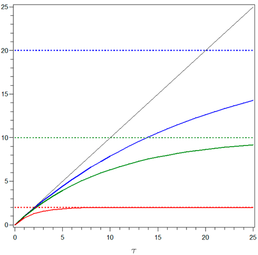
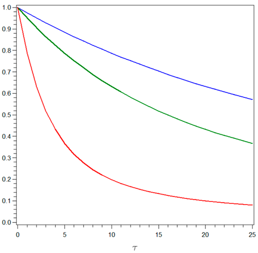
Hence, is equal to (minus) the semi-elasticity of the price with respect to x. It provides the percentage changes in the bond price attributable to an unexpected shift in the risk factor x and is then also referred to as the sensitivity of w.r.t. x. For this reason, is typically used as a measure of the real interest rate risk of the ZCB . is measured in time units, is zero for , and is monotonically increasing with . If (genuine mean-reversion), then for and has a horizontal asymptote at level ; the mean-reversion produces a ceiling on the interest rate risk. If (“mean repulsion”), then for and diverges for . The function for different values of is illustrated in the left figure of Table 1.

Table 1.
Functions and their horizontal asymptotes (left) and functions (right) for (blue lines), (green lines), and (red lines).
In our applications, it will be important to consider the variance of future values of the discount factors for . For the corresponding log-returns, we have, by (16),
where the conditional variance of , given by (6), depends on the parameters . As illustrated in the right figure of Table 1, for , the factor as a function of takes values in , is monotonically decreasing, and decreases more rapidly for increasing values of . This illustrates the important role that the risk-neutral mean-reversion plays in reducing the variability of returns and discount factors when the maturity changes.
2.3.4. Simulation of Future Prices and Rates
2.4. Introducing Money: The Two-Factor Model for the Price Index
Obviously, inflation effects can only occur when money is present in the economy. Therefore, to model inflation, we introduce money in this real market and denote by one unit of money (say, EUR 1). We denote by the price in units of money of one unit of the reference basket which defines the CPI. In this simple model, we assume that the introduction of money has no effects on the underlying equilibrium and money is only a measure of nominal value, that is, is simply the number of needed for receiving one at time t. However, this is sufficient for modeling nominal bonds.
Let us denote by the nominal value function at time t, that is, the market price expressed in EUR at time t. The general relation between nominal and real price is
because receiving one real unit, , at time t is equivalent to receiving nominal units, , at the same date. Let us consider the real value of a bond which provides with certainty the unit nominal payoff at maturity . Since, by relation (20), , to prevent arbitrage, the real value of this bond can be represented by
Then, for the nominal unit ZCB price , i.e., the money value at time t of one money unit at time T, we have, again by relation (20),
The same argument applies to more general nominal bonds. Therefore, in order to model nominal bond prices—or, equivalently, to model prices of the form —we have to extend the model for by making appropriate assumptions on the stochastic dynamics of .
2.4.1. The Two-Factor Model for the Price Index
We assume that the CPI is a diffusion process described by the following SDE:
with
Since , one has
Therefore, is the expected instantaneous rate of inflation at time t. If is deterministic, the CPI process is a geometric Brownian motion. However, in order to obtain a more realistic model, we assume that is also stochastic.
Our assumption is that the expected instantaneous inflation rate is a diffusion process described by the following SDE:
with
With this Vasicek specification, is also an Ornstein–Uhlembeck process.
As concerns the correlation structure, we assume
and
Assumptions (26) state the independence between real and nominal quantities and have important consequences. First of all, the form of the market risk premium is the same as in (12) and the market risk premia for the new two state variables are zero:
since property (11) also holds for the nominal quantities and and is a real quantity.
2.4.2. The Inflation Discount Factor and the Fisher Relation
Since the real payoff is independent of p and y, the price of real bonds is still obtained by the univariate model for . In particular, still has the Vasicek form (14).
As concerns , we have, by extension of (10):
where now the risk-neutral measure is three-dimensional. However, by the independence assumptions (26), we have
Hence,
For the expectation on the right-hand side, we observe that, since in the real economy, the risk premia and are set to zero, the relevant risk-neutral measure is equal to the natural probability measure. We define the folloing:
which will be referred to as the inflation discount factor on the time interval . Hence, we have
Expression (28) can be referred to as the Fisher relation in multiplicative form. As we shall see, since is stochastic, future expectations, i.e., for , are not known at time t. That is, like future real discount factors, future inflation discount factors too are stochastic.
2.4.3. The Expression for the Inflation Discount Factor
Let us define the CPI logarithmic price ratio on the time period :
Of course,
Using Result A3 in Appendix A.4, with and , for , the random variable is normal, with mean
and variance
where is given by with , that is,
It is important to note that these expressions are independent of the current level of the CPI. Furthermore, given the model parameters, the variance only depends on and the mean depends on t only through .
Using (31) and (32), an expression for is immediately obtained by computing the following moment-generating function:
We obtain
where is given by (33) and
For the inflation discount factor, the same properties already illustrated for the real discount factor hold; at time t, the inflation log-returns are affine functions of , and future values and , for , are, respectively, lognormally and normally distributed. Moreover, it is easily verified that
For the function given by (33), the same properties and the same interpretation hold as for . is a time measure of expected inflation risk, providing the sensitivity of the inflation discount factor to the risk factor . The only difference is that, being that is the natural risk reversion parameter, it is positive by assumption, so only the “capped” behavior (asymptote at ) is possible for ; the difference is strictly positive and monotonically increasing with .
2.4.4. Simulation of Future Rates and Prices
Also in this case, expression (35) allows us to easily simulate at time t future inflation discount factors as lognormal variables. More interesting for our applications, future values , , of the CPI are also simulated as lognormal, that is,
with standard normal. Taking account of (34), expression (38) can be also written as
This expression is important because if the discount factors can be observed in the market (as will be the case in our applications), future values of the CPI can be simulated in a market-consistent manner, i.e., consistent with the current market expectations on future inflation. This is equivalent to posing . In this case, since and do not enter into the expression of the variance , their observation or estimation is not required for the simulations of .
Remark 1.
In the two-factor model used in DFM23, where is deterministic, the risk-neutral inflation discount factor is defined as
where the expectation is taken w.r.t. the risk-neutral probability measure of the price process in the nominal economy setting and we use again the definition . However, in the two-factor model, one has , then , as in (30). Thus, the two models are formally consistent. Of course, in the three-factor model, the distribution of is more complex than in the case with deterministic expected inflation.
2.4.5. An “Economic” Derivation of the Inflation Discount Factor
Alternative derivations of expression (35) are available in the literature. We illustrate one which is interesting for its economic meaning. This derivation originates by the following observation. If we define a “new” Vasicek-type stochastic process , with drift parameters
the process is described by the following SDE:
By Result A2 in Appendix A.3, the stochastic integral is normal with mean
and variance
Then, it is easily verified that expression (35) can also be obtained as
The interesting point is that this is equivalent to saying
where is as in (37) and is the expectation taken with respect to a probability measure defined by the modified mean-reverting drift . By the Feynman–Kac theorem, this expression of is the solution, with terminal condition , of the following partial differential equation:
which has exactly the same form of the general valuation Equation (9) for the real ZCB price . As is shown in Appendix B, (43) is actually the general valuation equation for the discount factor in the nominal economy setting, i.e., when the security prices are measured in money units. In this setting, the market price of risk for the and factors are different from zero, and take exactly the form which determines the risk-adjusted drift and the modified process .3 Then is actually the risk-neutral measure in the nominal economy and is the corresponding expectation. These findings derive from the more general priciple that our pricing model can be reformulated in a nominal economy framework provided that the appropriate change of probability measure is made.
2.5. Nominal Interest Rates
By the Fisher relation (28) and expressions (14) and (35), we obtain the following closed-form expression for the nominal discount factor:
The instantaneous nominal interest rate is naturally defined as
with given in (29). Therefore, by (17) and (37), we obtain the Fisher relation for instantaneous returns:
Since depends on the two risk factors and , two different risk measures must be used:
where and are the real interest rate measure and the expected inflation risk measure previously defined.
Given the normality properties of and , is also normal, with mean equal to the sum of the means minus and, by the independence assumption, with variance equal to the sum of the variances. Given the normality of the exponent in (44), future nominal log-returns are normally distributed and future nominal ZCB prices are lognormally distributed.
3. Estimation of Model Parameters
3.1. Market Data
In order to estimate the parameters of the three-factor model, we used the same market data, by type and observation period, as in DFM23. This allows the results obtained with the three-factor model to be compared with those obtained with the two-factor model used in that paper.
- Price index process. As the reference CPI we choose the Harmonised Index of Consumer Prices (HICP), which is compiled by Eurostat and the euro-area national statistical institutes and is published at the end of each month.We use the monthly time series , where is the set of month-end dates in [January 2005, December 2022].
- Inflation discount factors. To estimate the parameters of the inflation component of the model, we use the Zero-Coupon Inflation-Indexed Swaps (ZCIIS). On each trading day t the ZCIIS rate is quoted on the market for time-to-maturity years. As shown in DFM23 (see also Brigo and Mercurio (2007)), the following no-arbitrage relations hold:Hence, provides the inflation discount factor prevailing on the market at time t for time-to-maturity .We use the daily time series , where is the set of trading days in [1 January 2005, 30 December 2022]. As a usual market practice, swap rates for the missing maturities in are computed by linear interpolation of quoted swap rates. Hence, at each date the swap rates are available for years. These maturities are usually sufficient for non-life actuarial applications.
- Nominal discount factors. Since the real discount factors are not directly observable on the market, we take data on the nominal risk-free discount factors, or rates, and then use the Fisher relation.In order to calibrate the model on the market at the valuation date 30 December 2022, we consider the risk-free nominal discount factors published by EIOPA. We choose the version including volatility adjustment. However, in order to obtain a complete estimate of the model, including the parameters of the natural probability measure, we also take the triple A yield curves computed by the European Central Bank (ECB) on each trading day (for details, see the Technical Notes downloadable from the ECB website European Central Bank (2023)). These curves are obtained by interpolating the observed returns on triple A bonds with different maturities using the Svensson model, a six-parameter smooth function. For the log-returns the Svensson function has the following form:with the parameter set (to avoid confusion, we have renamed the ECB parameters and as and , respectively). Observe that . Thus, with this interpolating function there is no problem in determining the initial point of the yield curve. Differently from DFM23, where only the parameters are required, we use the daily time series of the entire parameter sets estimated by ECB. The corresponding yield curves are denoted by and the instantaneous interest rates as .4
For further details and illustrations, see De Felice and Moriconi (2023). In particular, Figure 1 in that paper shows the yield curves as well as the risk-neutral market expectations of the future annual inflation rates:
for up to 25 years. In our three-factor model, however, the risk-neutral market expectations are equal to the natural expectations of future inflation rates.
3.2. Parameters of the Inflation Component
Our aim in this section is to derive an estimate of the parameters of the CPI distribution, including the instantaneous expected inflation rate, which is not directly observable. In a first step we estimate and , then we estimate and , and finally, we provide an estimate of and for all .
3.2.1. Time Series Estimate of and
We consider the time series of market inflation log-returns for and . As a first step of the estimation procedure, we estimate and on the time series of the one-year log-returns . In principle, a time series of instantaneous inflation rates would be needed. However, is not directly observable and should be extrapolated by observed returns over finite time periods. Since an appropriate extrapolation function is not available at this stage, we defer to Section 3.2.3 the estimate of a time series of instantaneous inflation rates and consider here directly the market log-returns for one-year time-to-maturity. The rationale is that should be the observed inflation rate for which the correlation with the instantaneous rate is highest.5
We use the affinity property of the log-returns. We rewrite expression (35) as
with
where is given by (36). Then we can write
with
By Ito’s lemma, we have the following SDE for (where we omit the dependence on ):
Since, by (48), we obtain
or
with
Observe that, since , then ; hence, .
As shown in Appendix A.2, for a chosen time-to-maturity and a chosen time step , (51) corresponds to the following first-order autoregressive model:
where the error terms are independent with zero mean and variance . Using the time series of market values , the parameter estimates , and are obtained by linear regression and the corresponding estimate of the mean-reversion coefficient is given by
Then we obtain
This estimation procedure can be applied for any value of for which market observations are available. However, as previously noticed, the most reliable results should be that obtained for year. The corresponding estimation procedure (assuming 260 trading days per year, that is, ) provided the following results:
Remark 2.
The illustrated estimation procedure is viable because in our model, the inflation market risk premium is independent of , and hence the mean-reversion coefficient is the same under the natural and the risk-neutral measure. This approach could not be directly applied to , since the time series estimate allows us to obtain the real-world parameter , while depends on its risk-adjusted version .
3.2.2. Time Series Estimate of and
From the monthly time series of HICP values observed at each month-end in [January 2005, December 2023], we derived the time series of monthly log-price-ratios ():
We show how and can be estimated in our model considering this time series and a corresponding time series of stochastic integrals.
Let us consider the two random variables and . For chosen , these variables are normal and, using expression (A22) in Appendix A.4 (with the usual specifications and ), we have
where, by expression (A21),
Therefore, can be obtained as
and, in turn, is given by
Since is not observable, we use
for a given (which, for the same reasons illustrated in Section 3.2.1, should be 1 year). By (48), and ; hence,
and
The variance and the covariance can be estimated on a monthly () time series of CPI log-price-ratios and a corresponding monthly time series , where
with , and n represents the number of trading days in each month. The estimates obtained in the previous section were used for and .
This estimation procedure provided the following results:
3.2.3. Estimate of and on a Time Series of Cross-Sections
Having estimated the parameters , and , our model provides an appropriate extrapolation procedure that allows us to estimate the instantaneous inflation rate , together with the parameter , by a regression on an observed cross-section of log-returns . Since these returns are affine functions of , by some manipulations, this estimation procedure takes the form of a linear regression.
Then, defining as the dependent variable and
as the independent variables, we are led to the following two-dimensional linear model (without intercept):
with the usual assumptions on the error terms .
For the estimation at the valuation date t, the data for the dependent variable are the cross-section , where is computed using the parameter estimates previously derived. However, we need not only an estimate at time 30 December 2022, but also an estimate for each , i.e., at each date of the time series. So, we repeated the linear regression estimate (56) for each cross-section , , thus obtaining the time series of estimated values . These estimates are illustrated in Figure 1.
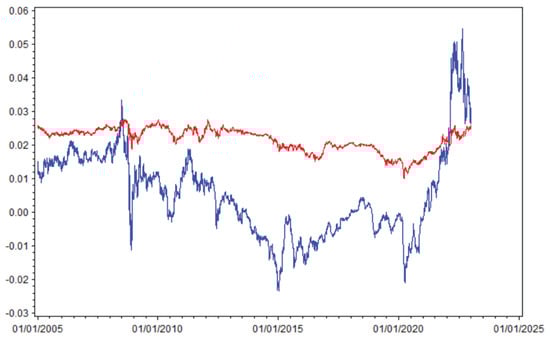
Figure 1.
Daily cross-sectional estimates of (blue line) and (red line).
Remark 3.
Of course, a parameter different for each time point is clearly inconsistent with the model assumptions. However, this forcing of the assumptions is only used here to obtain an extrapolation function not too inconsistent with the model. On the other hand, our model for the inflation discount factors is too simple to capture the market dynamics well enough to produce constant parameter estimates across any observation date. We point out, however, that, since in Section 3.3.3 we will calibrate the real discount factors on the observed term structure of real interest rates using the Hull and White model, the estimates of will not be used.
3.3. Parameters of the Real Interest Rate Component
In this section, we estimate both the natural and the risk-neutral parameters of real interest rate component of the model, introduced in Section 2.2 and Section 2.3.
3.3.1. Derivation of Real Interest Rate Data by Nominal Interest Rate Data
By the estimated Svensson parameters published each trading day by ECB, we computed the risk-free nominal log-returns according to (46) and then derived the corresponding real log-returns using the Fisher relation:
The Fisher relation was also used to derive the corresponding time series of estimated real instantaneous interest rates:
where is estimated in the previous section and in Section 3.2.2. The time series of these estimated instantaneous rates are illustrated in Figure 2.
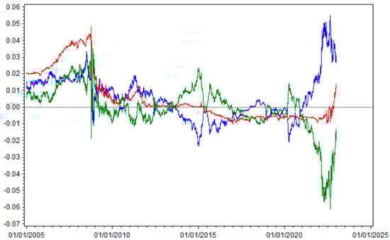
Figure 2.
Daily estimates of (blue), (red), and (green line).
3.3.2. Time Series Estimate of Natural Real Interest Rate Parameters
In order to estimate the real-world parameters of the real interest rate process introduced in Section 2.2, we applied to the time series the classical OU estimators just used in Section 3.2.1. This estimation procedure provided the following results:
By the independence assumption, .
3.3.3. Calibration of the Real Interest Rate Model
To simulate at the valuation date t the future real discount factors , , we have to calibrate the real interest rate model on time t data. In order to obtain a perfect fit to the term structure derived from the market data, we used the extension of Vasicek’s model provided by Hull and White (Hull and White 1990). The details of this model are given in Appendix C. As shown in the appendix, the Hull–White estimates of future discount factors , for , are computed as
where is normal with mean zero and variance
and
with
The sensitivity function in (59) has the usual form .
The parameters and have already been estimated (as and ). It therefore remains to estimate the risk-neutral mean-reversion parameter . In DFM23, where the same problem arises for the calibration of nominal interest rates, this was accomplished by a best-fitting procedure of the model yield function to the current market term structure . This procedure applied to our real interest rate data has proven to be scarcely reliable, producing rather unstable estimates of . We therefore found it convenient to perform the estimation using the entire time series of cross-sections for . Using the affinity property of as we did in Section 3.2.1 for the inflation discount factor , we are led to the following SDE for the real log-returns, which is the analogue of (51):
The coefficients a and b, which have the same form as in (52), are known at time t. Thus, we have
These variances are independent of t. For a sufficiently small finite time interval , we can consider the following approximations:
We derived a time series estimate of these variables for by taking the sample variance of the daily increments:
and we thus obtained an estimate of by solving the ordinary-least-squares problem:
We obtained .
4. Applying the Market Model to Claims Reserving
4.1. The Essential Elements of the Claims Reserving Application
For the claims reserving applications of the model, we adopt the definitions, theoretical framework, and simulation schemes proposed in DFM23. However, we do not consider the “actuarial approach”, which is characterized by the exclusion of interest rate risk. As also noted in DFM3, if we accept this approximation, it would not make sense to use a stochastic model for interest rates, much less one with stochastic expected inflation. Therefore, here we will only consider the so-called “market approach” and remove the superscript M used in the DFM23 notation when it is necessary to distinguish this approach from the actuarial approach (denoted there by the superscript A). We recall here for convenience the essential definitions introduced in DFM23.
The chain-ladder reserve at the current date , the end of year 2022, is given by
where
- the superscript cc indicates that the chain-ladder algorithm is applied to a triangle of claim payments expressed at current costs, i.e., adjusted for the past inflation as measured by the HICP index (the CPI to which the ZCIIS are linked);
- denotes the chain-ladder estimate at time I of the sum of the incremental payments (at time I costs) to be performed in the k-th future calendar year.
Of course, are the current market real discount factors, computed as , where are the risk-free discount factors provided at time I by EIOPA (including volatility adjustment) and are the inflation discount factors derived by the ZCIIS observed at time I.
As regards reserve risk under the ultimate point of view, the predictive distribution of the discounted ultimate obligations (DUOs) provided by S simulations is given by
It is assumed that the claim payments are provided by the bootstrap simulation of a chosen stochastic chain-ladder model. Under the short-term view of reserve risk, as prescribed by Solvency II, the predictive distribution of the year-end obligations (YEOs) is given by
where the residual reserve at time in the s-th simulation is given by
Here, are the real discount factors at time simulated consistently with the current term structure using the Hull and White Formula (59) and the price index at time is simulated as suggested in Section 2.4.4 using expression (39). The inflation discount factors derived by the ZCIIS quoted in the market represent, by definition, risk-neutral expectations. However, in the three-factor model, we have , since the risk premia and are zero. So, in effect, expression (39) is written as
Remark 4.
In the two-factor model (see Section 4.2 in DFM23), the expression corresponding to (39) is
But in that model, the natural and the risk-neutral measures are different and the relation holds as . Thus, we obtain a relation formally identical to (62). This means that in the two models, the market data are used in the same way. Of course, as already pointed out, the expression of is different in the two models. However, it is immediately verified that if in the three-factor model we set , i.e., if we make expected inflation deterministic, we obtain , as in the two-factor model.
4.2. Numerical Results with the Market Approach
For the numerical calculations, we used the same triangle of paid losses used in DFM23, which contains the MTPL claim payments observed at the end of 2022 (time I) over the previous 22 accident years (so the data also include the period of the COVID-19 pandemic). As in that paper, the stochastic chain-ladder model used is the ODP reserving model introduced by Renshaw and Verral (1998), in the bootstrap version proposed by England and Verral (2002). Since the definitions of the quantities to be estimated, the market data and the paid losses data, are the same in the two articles, the differences in the results obtained can only be attributed to the difference in the market model used and the estimates of the relevant parameters.
4.2.1. Recall of Results with the Two-Factor Model
In DFM23, the results of the market approach are as follows (see the paper for further details):
| Results with deterministic computations | |
| - Undiscounted reserve with implicit inflation | 100,000 |
| - Discounted reserve with implicit inflation: | 91,091 |
| - Undiscounted reserve with triangle at current costs: | 100,087 |
| - Discounted reserve with triangle at current costs: | 91,391 |
| - Undiscounted reserve with modeled inflation | 109,445 |
| - Discounted reserve with modeled inflation (BE): | 99,402 |
| Results with the two-factor model (100,000 simulations) | |
| - DUO sample mean: | 99,304 |
| - DUO Std | 5101 |
| - DUO CV | 5.14% |
| - YEO sample mean: | 102,809 |
| - YEO Std | 4773 |
| - YEO CV | 4.64% |
| - percentile of YEO | 115,880 |
| - Solvency Capital Requirement | 13,071 |
| - Present value of YEO sample mean: | 99,461 |
4.2.2. Using the Three-Factor Model
Using the three-factor model, the deterministic results are obviously the same. The results on reserve risk under the ultimate point of view also do not change, as the discount factors used in expression (60) are those observed on the market. For the reserve risk under the one-year view, the results are different, however.
| Results with the three-factor model (100,000 simulations) | |
| - YEO sample mean: | 102,762 |
| - YEO Std | 4950 |
| - YEO CV | 4.82% |
| - percentile of YEO | 116,314 |
| - Solvency Capital Requirement | 13,551 |
| - Present value of YEO sample mean: | 99,416 |
While the YEO sample mean and its discounted value are the same, within the Monte Carlo error, as in the two-factor model, the introduction of stochastic expected inflation in the valuation model produces a non-negligible increase in the variability of the predictive loss distribution. The coefficient of variation increases from to , and the SCR, as a percentage of the BE, increases by about 50 basis points, from to . These increases are roughly similar to those found in DFM23 when passing from the actuarial approach to the market approach with the two-factor model.
With regard to the kurtosis of the predictive distribution and the relationships with the corresponding moment-fitted lognormal distribution, there are no relevant differences to what was found with the two-factor model.
4.2.3. The Determinants of the Increase in Variability
It may be of some interest to analyze the determinants of the increase in variability produced by the model with stochastic expected inflation. The variance of the empirical distribution defined in (61) is determined by the variance of the one-year repricing factor and the year-end real discount factors , . Expression (61) applies to both the tree-factor model and the two-factor model in DFM23, the only difference being in the way these factors are calculated. Let us introduce the shorthand notation for , for , and for the product , and let us denote by , and the corresponding standard deviations. In the three-factor model, depends on the parameters through the relation (39) and the expression (32) of , and depends on the parameters entering the Hull–White expression (59) of . In particular, and determine the variance of . In the two-factor model, depends on the parameter and depends on the parameters in the Hull–White expression of the nominal discount factors analogous to (59) (expression (32) in DFM23). For these parameters, the estimates derived in DFM23 are
while with the three-factor model, we derived in the previous sections
Thus, volatilities are higher in the three-factor model than in the two-factor model, but so are the mean-reversion parameters, both natural and risk-neutral. Since, as we have seen, mean-reversion produces a decrease in variability for increasing maturities, it is useful to compare the combined effect of these parameter values. This can be easily carried out, since the standard deviations of the factors involved in (61) can be computed in closed form, using the relation , valid for . The results of the computations are reported in Figure 3, where the standard deviations for different maturities are illustrated in blue color for the three-factor model and in red for the two-factor model. It can be seen that, although the standard deviation of is larger in the three-factor than in the two-factor model, the standard deviations of the discount factors in the three-factor model are smaller even before the 2-year maturity. The change in dominance is even more evident when looking at the overall standard deviations, indicated by continuous lines, where the crossing of the curves occurs for a maturity between 3 and 4 years. Since by far the largest portion of the year-end obligations have maturity of less than 3 years, the variability of the overall present value is greater for the blue curve than for the red curve. That is, we have an increase in SCR with the three-factor model.
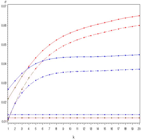
Figure 3.
Standard deviations of the stochastic factors and in the three-factor model (blue lines) and the two-factor model (red lines), as a function of the time-to-maturity k. The dashed lines represent and the continuous lines represent the overall volatility in the two models. The dotted lines indicate the level of the standard deviation of .
5. Conclusions
When simulating the distribution of year-end obligations, we find with our data that the three-factor model produces higher volatility than the two-factor model for both the repricing factor of the CPI and the next-year real discount factors to be applied to the claim payments of the remaining calendar years. However, the mean-reversion, both natural and risk-neutral, of real interest rates in the three-factor model is also higher than that derived from nominal interest rates in the two-factor model. This may cause the overall volatility of the three-factor model to be lower over long maturities. In our case, the overall effect is that, with the market approach of the three-factor model, the reserve SCR (under the one-year view) has a non-negligible increase over that derived with the market approach of the two-factor model. This increase is grosso modo similar to that found in DFM23 when switching from the actuarial to the market approach in the two-factor model.
Funding
This research received no external funding.
Acknowledgments
The author would like to thank Luca Passalacqua for the useful discussions on the development and the estimation of the three-factor model presented in this paper.
Conflicts of Interest
The author declares no conflict of interest.
Abbreviations
The following abbreviations are used in this manuscript:
| BE | Best Estimate |
| DFM23 | De Felice and Moriconi (2023) paper |
| HICP | Harmonised Index of Consumer Prices |
| SCR | Solvency Capital Requirement |
| SDE | Stochastic Differential Equation |
| ZCB | Zero-Coupon Bond |
| ZCIIS | Zero-Coupon Inflation-Indexed Swap |
Appendix A. Some Fundamental Results on Ornstein–Uhlembeck Process
Appendix A.1. Integral Representation of the Ornstein–Uhlembeck Process
Let be the OU process described by the SDE:
As is well-known, this is a shorthand expression for the following integral representation:
(where the stochastic integral is defined in Ito’s sense). We prove the following fundamental result concerning the conditional random variable .
Result A1.
For , we have
with
Therefore,
where the conditional mean is
with
hence depending only on and , and the conditional variance is
which depends only on .
Proof.
We first apply a transformation providing an SDE with constant drift. Let . Differentiating:
Then is described by the following SDE:
For ,
Replacing with , we then have
This gives expression (A2), with given by (A3) and given by (A4). Expression (A5) is immediately obtained by the following property:
which gives
□
Appendix A.2. Parameter Estimate for the Ornstein–Uhlembeck Process
Taking and interpreting expression (A6) as an iterative relation, we see that the discrete equivalent of the SDE (A1) is the first-order autoregressive equation:
with
and where the error terms are independent normal with zero mean and constant variance
If a time series of observations of with time step is available, the standard linear regression defined by (A8) provides the corresponding consistent estimates , and . By (A9)–(A11), we obtain
If time is measured in years and we have a daily (weekly, monthly) time series, then we pose (, resp.). Consequently, all the estimates will be consistently expressed on annual basis.
Appendix A.3. Integral of the Ornstein–Uhlembeck Process
For , let us consider the stochastic integral:
with described by (A1). The following fundamental result holds for the conditional random variable .
Result A2.
For we have
with given by (A3) and
Hence,
with conditional mean
which depends only on and , and conditional variance
which depends only on .
Proof.
The normality of is an obvious consequence of the normality of . Expression (A14) is obtained by integrating in (A4). The stochastic term in (A13) is obtained by integrating in (A3). In fact, we have (using Fubini’s theorem)
Expression (A15) for the variance can be obtained by computing the following integral:
Appendix A.4. Log-Returns of the Price Index Process
Let us consider the process defined by the following SDE:
with given by (A1) and . Let us define the “log-return”, i.e., the logarithm of the price ratio, on the time period :
We prove the following fundamental result for the random variable .
Result A3.
For , we have
with
and independent. Then
with conditional mean
which depends only on and , and conditional variance
which depends only on .
Proof.
We rewrite the stochastic dynamics of using a Cholesky decomposition of the bivariate Wiener process . This gives
where and are independent Wiener processes. By the second SDE in (A20), we have, applying Ito’s lemma,
The solution of this SDE for , given , is
For the log-price-ratio , we then have
which is obviously normal. Expression (A18) is immediately obtained, since , with given by (A14). Expression (A19) is easily proven considering that, by (A13),
Then, by the independence of and :
That is,
where we used (A16). Since , as in (A7), expression (A19) is obtained. □
Appendix B. The General Valuation Equation in the Nominal Economy
Let us consider at time t a real ZCB which provides at time a real payoff which is defined as a specified function contractually specified of and . Then the price of this bond is a function of all three risk factors. By the hedging argument, is obtained as the solution of the following general valuation equation:
with terminal condition . By the Feynman–Kac theorem, this solution is given by
where is taken with respect to the three-dimensional risk-neutral distribution . The valuation Equation (9) and the corresponding solution for , given by (14) after has been specified as in (12), is immediately obtained as a particular case of (A23) if one requires , since in this case, only depends on .
If we skip to the corresponding nominal economy setting, the general valuation equation for the nominal price is derived by Equation (A23) by posing and computing the corresponding derivatives. Making the calculations and rearranging, we obtain
or
with
These expressions for the nominal risk premia for y and p can also be obtained by computing the corresponding covariance w.r.t. the nominal wealth . This is carried out in a footnote in Section 2.4.5.
Let us specify the price as the price of the nominal unit ZCB maturing at time T. By the Fisher relation we know that , where depends only on x. By the independence assumption, is independent of x. Moreover, as shown in Section 2.4.3, is also independent of p. Hence, we have . As a consequence of this separation property, the nominal valuation Equation (A24) provides two separated equations, one for , corresponding again to Equation (9), and the other for u, having the following form:
Using our specifications for and , we have
with . Since deriving with respect to is the same as deriving with respect to y, this equation can be written as
or
with . The solution of this equation, under terminal condition , is given by , which gives (42).
Appendix C. Applying the Hull and White Model
This section largely mimics Appendix B in DFM23. In order to have a perfect fit to the market discount factors at the valuation date, we consider the Hull and White extension of the Vasicek model for the process (Hull and White 1990). As usual, can be interpreted as or in the main text of the paper. Correspondingly, the discount factor v which will be used in this appendix can be interpreted as or u, respectively. In Section 3.3.3, the first interpretation is used.
In the Hull and White model, the long-term rate is assumed to be time-dependent and is expressed by
where is the following OU process:
and is a deterministic function with . Time 0 is the reference date when z and are equal and it is also the date where we observe on the market the discount factors for . For our aim is to derive an expression which for perfectly fits the observed term structure .
In this model, we have
where the expectation is taken w.r.t. the appropriate risk-neutral measure. By the usual calculations, we obtain
with
and
Hence,
We also obtain
Therefore,
with
For we have , and ; therefore, since , (A25) provides , i.e., perfect fitting, as desired.
At time 0, the future discount factor , with , is lognormal, with moments (under the natural distribution):
since , and:
Therefore computation of expectation only requires the risk-adjusted parameter , while for the computation of variance both and are required.
It can be shown that if these moments are computed under the risk-neutral measure the corresponding expressions fulfil the theoretical property .
Notes
| 1 | To simplify notation we shall denote by , where is a random variable depending on the sample path in of a given stochastic process , the conditional expectation of given , where is the -field generated by up to time t. |
| 2 | Actually, in this risk-neutral setting we may not have real mean-reversion, because could be negative. |
| 3 | This is immediately seen by observing that in the nominal economy the optimally allocated wealth is measured in money unit and is then given by . Since the market risk premia are given by the covariance of changes in the relevant risk factor with percentage changes in , we obtain:
|
| 4 | The ECB risk-free yield curves are slightly different from the yield curves provided by EIOPA, since EIOPA yield curves are primarily derived from observed interest rate swaps (after appropriate adjustment for credit risk), inter/extrapolated by the Smith-Wilson method. However, these differences have little relevance to our estimation problem. |
| 5 | As it is well-known, in a one-factor model rates of return of different maturities are perfectly correlated. This property is clearly unrealistic, but could be considered acceptable for maturities that are very close to each other. |
References
- Brigo, Damiano, and Fabio Mercurio. 2007. Interest Rate Models: Theory and Practice. With Smile, Inflation and Credit, 2nd ed. New York: Springer. [Google Scholar]
- Cox, John C., Jonathan E. Ingersoll, and Stephen A. Ross. 1985. A theory of the term structure of interest rates. Econometrica 53: 385–406. [Google Scholar] [CrossRef]
- De Felice, Massimo, and Franco Moriconi. 2023. Stochastic Chain-Ladder Reserving with Modeled General Inflation. July 21. Available online: https://ssrn.com/abstract=4517501 (accessed on 5 October 2023). [CrossRef]
- England, Peter D., and Richard J. Verrall. 2002. Stochastic Claims Reserving in General Insurance (with discussion). British Actuarial Journal 8: 443–544. [Google Scholar] [CrossRef]
- European Central Bank. 2023. Technical Notes on ECB Yield Curve Methodology. Available online: https://www.ecb.europa.eu/stats/financial_markets_and_interest_rates/euro_area_yield_curves/shared/pdf/technical_notes.pdf (accessed on 5 October 2023).
- Hull, John, and Alan White. 1990. Pricing Interest Rate Derivative Securities. Review of Financial Studies 3: 573–92. [Google Scholar] [CrossRef]
- Jarrow, Robert, and Yildiray Yildirim. 2003. Pricing Treasury Inflation Protected Securities and Related Derivatives using an HJM Model. Journal of Financial and Quantitative Analysis 38: 337–58. [Google Scholar] [CrossRef]
- Moriconi, Franco. 1995. Analyzing default-free bond markets by diffusion models. In Financial Risk in Insurance. Edited by Giuseppe Ottaviani. Berlin: Springer. [Google Scholar]
- Renshaw, Arthur E., and Richard J. Verrall. 1998. A stochastic model underlying the chain ladder technique. British Actuarial Journal 4: 903–23. [Google Scholar] [CrossRef]
- Vasicek, Oldrich. 1977. An equilibrium characterization of the term structure. Journal of Financial Economics 5: 177–88. [Google Scholar] [CrossRef]


Disclaimer/Publisher’s Note: The statements, opinions and data contained in all publications are solely those of the individual author(s) and contributor(s) and not of MDPI and/or the editor(s). MDPI and/or the editor(s) disclaim responsibility for any injury to people or property resulting from any ideas, methods, instructions or products referred to in the content. |
© 2023 by the author. Licensee MDPI, Basel, Switzerland. This article is an open access article distributed under the terms and conditions of the Creative Commons Attribution (CC BY) license (https://creativecommons.org/licenses/by/4.0/).