
GARMA, HAR and Rules of Thumb for Modelling Realized Volatility

Abstract
:1. Introduction
2. Previous Work and Econometric Models
2.1. The Basic GEGENBAUER Model
- where represents the short-memory autoregressive component of order
- represents the short memory moving average component of order
- represents the long-memory Gegenbauer component (there may in general be k of these),
- represents integer differencing (currently only = 0 or 1 is supported),
- represents the observed process,
- represents the random component of the model—these are assumed to be uncorrelated but identically distributed variates,
- represents the Backshift operator, defined by
2.2. Heterogenous Autoregressive Model (HAR)
2.3. Historical Volatility Model (HISVOL)
3. Results
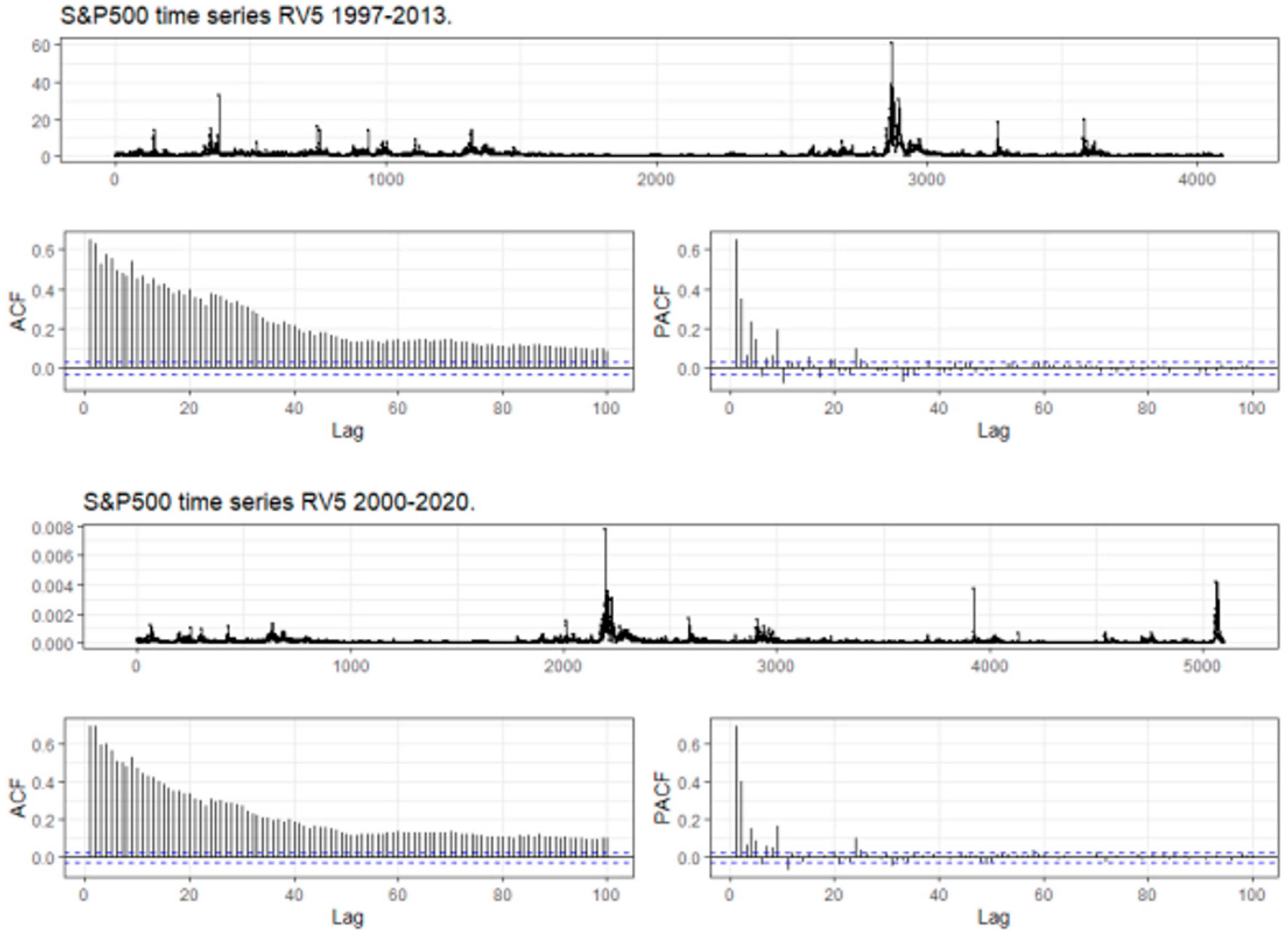
3.1. The Data Sets
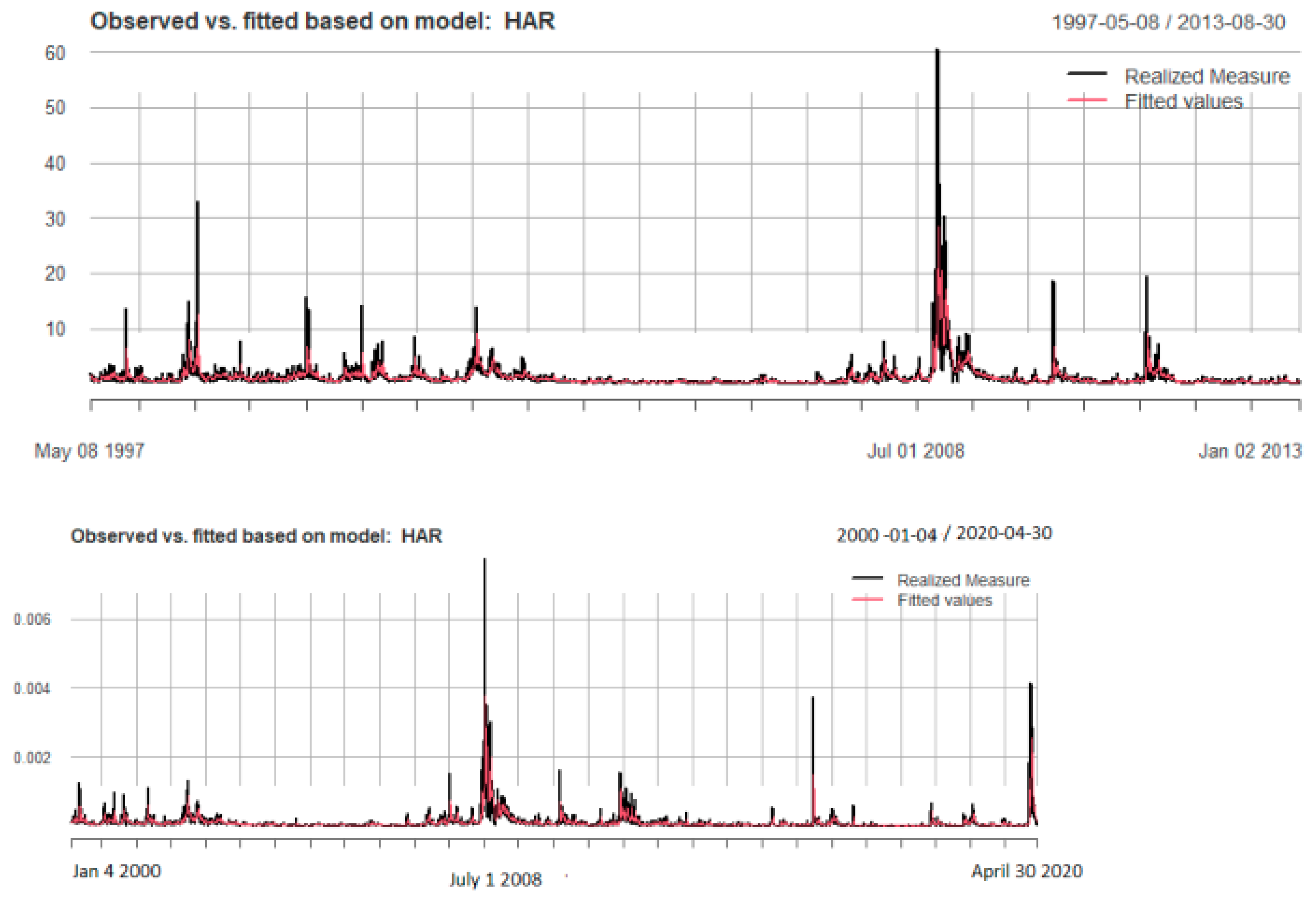
3.2. The Basic HAR Model
3.3. Gegenbauer Results
3.4. How Do Rule of Thumb Approaches Perform?
- Identifies the right subset model, {j: j≠ 0} = A
- Has the optimal estimation rate, √n ((δ)A − β*A) → d N(0,Σ*), where Σ* is the covariance matrix knowing the true subset model.
4. Conclusions
Author Contributions
Funding
Data Availability Statement
Conflicts of Interest
References
- Allen, David E., and Michael McAleer. 2020. Do we need stochastic volatility and Generalised Autoregressive Conditional Heteroscedasticity? Comparing squared end-of-day returns on FTSE. Risks 8: 12. [Google Scholar] [CrossRef]
- Allen, David Edmund. 2020. Stochastic volatility and GARCH: Do squared end-of-day returns provide similar information? Journal of Risk and Financial Management 13: 202. [Google Scholar] [CrossRef]
- Anděl, Jiří. 1986. Long memory time series models. Kybernetika 22: 105–23. [Google Scholar]
- Andersen, Torben G., Tim Bollerslev, Francis X. Diebold, and Heiko Ebens. 2001. The distribution of realized stock return volatility. Journal of Financial Economics 61: 43–76. [Google Scholar] [CrossRef]
- Andersen, Torben G., Tim Bollerslev, Francis X. Diebold, and Paul Labys. 2003. Modeling and forecasting realized volatility. Econometrica 71: 529–626. [Google Scholar] [CrossRef]
- Barndorff-Nielsen, Ole E., and Neil Shephard. 2002. Econometric analysis of realised volatility and its use in estimating stochastic volatility models. Journal of the Royal Statistical Society, Series B 63: 253–80. [Google Scholar] [CrossRef]
- Barndorff-Nielsen, Ole E., and Neil Shephard. 2003. Realized power variation and stochastic volatility models. Bernoulli 9: 243–65. [Google Scholar] [CrossRef]
- Bollerslev, Tim. 1986. Generalized Autoregressive Conditional Heteroscedasticity. Journal of Econometrics 31: 307–327. [Google Scholar] [CrossRef]
- Box, George E. P., and Gwilym M. Jenkins. 1970. Times Series Analysis. Forecasting and Control. San Francisco: Holden-Day. [Google Scholar]
- Christensen, Bent J., and Nagpurnanand R. Prabhala. 1998. The relation between implied and realized volatility. Journal of Financial Economics 37: 125–50. [Google Scholar] [CrossRef]
- Commandeur, Jacques J. F., and Siem Jan Koopman. 2007. Introduction to State Space Time Series Analysis. Oxford: Oxford University Press. [Google Scholar]
- Corsi, Fulvio. 2009. A simple approximate long-memory model of realized volatility. Journal of Financial Econometrics 7: 174–96. [Google Scholar] [CrossRef]
- Dacorogna, Michel M., Ulrich A. Muller, Richard B. Olsen, and Olivier V. Pictet. 1998. Modelling short term volatility with GARCH and HARCH. In Nonlinear Modelling of High Frequency Financial Time Series. Edited by C. Dunis and B. Zhou. Chichester: Wiley. [Google Scholar]
- Dickey, David A., and Wayne A. Fuller. 1979. Distribution of the Estimators for Autoregressive Time Series with a Unit Root. Journal of the American Statistical Association 74: 427–31. [Google Scholar]
- Dissanayake, G. S., M. Shelton Peiris, and Tommaso Proietti. 2018. Fractionally Differenced Gegenbauer Processes with Long Memory: A Review. Statistical Science 33: 413–26. [Google Scholar] [CrossRef]
- Dissanayake, Gnanadarsha Sanjaya. 2015. Advancement of Fractionally Differenced Gegenbauer Processes with Long Memory. Ph.D. thesis, School of Mathematics and Statistics, University of Sydney, Sydney, NSW, Australia. [Google Scholar]
- Efron, Bradley, Trevor Hastie, Iain Johnstone, and Robert Tibshirani. 2004. Least Angle Regression. The Annals of Statistics 32: 407–99. [Google Scholar] [CrossRef]
- Engle, Robert F. 1982. Autoregressive conditional heteroskedasticity with estimates of the variance of United Kingdom inflation. Econometrica 50: 987–1007. [Google Scholar] [CrossRef]
- Engle, Robert F., and Clive W. J. Granger. 1987. Co-integration and error correction: Representation, estimation and testing. Econometrica 55: 251–76. [Google Scholar] [CrossRef]
- Fan, Jianqing, and Runze Li. 2001. Variable Selection via Nonconcave Penalized Likelihood and Its Oracle Properties. Journal of the American Statistical Association 96: 1348–60. [Google Scholar] [CrossRef]
- Granger, Clive W. J., and Roselyne Joyeux. 1980. An introduction to long-memory time series models and fractional differencing. Journal of Time Series Analysis 1: 15–29. [Google Scholar] [CrossRef]
- Gray, Henry L., Nien-Fan Zhang, and Wayne A. Woodward. 1989. On generalized fractional processes. Journal of Time Series Analysis 10: 233–57, Erratum in Journal of Time Series Analysis 15: 561–62. [Google Scholar] [CrossRef]
- Guegan, Dominique. 2000. A new model: The k-factor GIGARCH process. Journal of Signal Processing 4: 265–71. [Google Scholar]
- Hosking, J. R. M. 1981. Fractional differencing. Biometrika 68: 165–76. [Google Scholar] [CrossRef]
- Hunt, Richard. 2022a. Garma: Fitting and Forecasting Gegenbauer ARMA Time Series Models, R Package Version 0.9.11. Available online: https://CRAN.R-project.org/package=garma (accessed on 3 October 2023).
- Hunt, Richard. 2022b. Investigations into Seasonal ARMA Processes. Ph.D. thesis, School of Mathematics and Statistics, University of Sydney, Sydney, NSW, Australia. [Google Scholar]
- Hunt, Richard, Shelton Peiris, and Neville Weber. 2021. Estimation methods for stationary Gegenbauer processes. Statistical Papers 63: 1707–41. [Google Scholar] [CrossRef]
- Peiris, M. Shelton, and Manabu Asai. 2016. Generalized fractional processes with long memory and time dependent volatility revisited. Econometrics 4: 37. [Google Scholar] [CrossRef]
- Peiris, Shelton, David Allen, and Udara Peiris. 2005. Generalised autoregressive models with conditional heteroscedasticity: An application to financial time series modelling. In The 2004 Workshop on Research Methods: Statistics and Finance, Proceedings of the 2004 Workshop on Research Methods: Statistics and Finance. Edited by Eric J. Beh, Robert G. Clark and J. C. W Rayner, Wollongong: University of Wollongong, pp. 75–83. ISBN 1 74128 107 5. [Google Scholar]
- Peiris, M. Shelton, and Aera Thavaneswaran. 2007. An introduction to volatility models with indices. Applied Mathematics Letters 20: 177–82. [Google Scholar] [CrossRef]
- Perron, Pierre, and Wendong Shi. 2020. Temporal aggregation and Long Memory for asset price volatility. Journal of Risk and Financial Management 13: 181. [Google Scholar] [CrossRef]
- Phillip, Andrew. 2018. On Gegenbauer long memory stochastic volatility models: A Bayesian Markov chain Monte Carlo approach with applications. Ph.D. thesis, School of Mathematics and Statistics, University of Sydney, Sydney, NSW, Australia. [Google Scholar]
- Poon, Ser-Huang, and Clive Granger. 2005. Practical issues in forecasting volatility. Financial Analysts Journal 61: 45–56. [Google Scholar] [CrossRef]
- Poterba, James M., and Lawrence H. Summers. 1986. The persistence of volatility and stock market fluctuations. American Economic Review 76: 1124–41. [Google Scholar]
- Ramsey, James Bernard. 1969. Tests for Specification Errors in Classical Linear Least Squares Regression Analysis. Journal of the Royal Statistical Society, Series B 31: 350–71. [Google Scholar] [CrossRef]
- Schreiber, Sven. 2023. adalasso.gfn GRETL Code Function. Available online: https://gretl.sourceforge.net/cgi-bin/gretldata.cgi?opt=SHOW_FUNCS (accessed on 3 October 2023).
- Schwert, G. William. 1989. Why does stock market volatility change over time? Journal of Finance 44: 1115–53. [Google Scholar] [CrossRef]
- Shephard, Neil, and Kevin Sheppard. 2010. Realising the future: Forecasting with high-frequency-based volatility (HEAVY) models. Journal of Applied Econometrics 25: 197–231. [Google Scholar] [CrossRef]
- Sjoerup, Emil. 2019. HARModel: Heterogeneous Autoregressive Models. R Package Version 1.0. Available online: https://CRAN.R-project.org/package=HARModel (accessed on 3 October 2023).
- Slutsky, Eugen. 1927. The summation of random causes as the source of cyclic processes. Econometrica 5: 105–46. [Google Scholar] [CrossRef]
- Taylor, Stephen J., and Xinzhong Xu. 1997. The incremental volatility information in one million foreign exchange quotations. Journal of Empirical Finance 4: 317–40. [Google Scholar] [CrossRef]
- Tibshirani, Robert. 1996. Regression Shrinkage and Selection via the Lasso. Journal of the Royal Statistical Society, Ser. B 58: 267–88. [Google Scholar] [CrossRef]
- Whittle, Peter. 1953. The analysis of multiple stationary time series. Journal of the Royal Statistical Society. Series B (Methodological) 15: 125. [Google Scholar] [CrossRef]
- Yule, G. Udny. 1926. Why do we sometimes get nonsense correlations between timeseries? A study in sampling and the nature of time-series. Journal of the Royal Statistical Society 89: 1–63. [Google Scholar] [CrossRef]
- Zou, Hui. 2006. The Adaptive Lasso and Its Oracle Properties. Journal of the American Statistical Association 101: 1418–29. [Google Scholar] [CrossRef]

| Descriptor | S&P500 1997–2013 | S&P500 2000–2020 |
|---|---|---|
| Number of Observations | 4096 | 5099 |
| Minimum | 0.04329 | 0.00000122 |
| Maximum | 60.56 | 0.0074 |
| median | 0.6294 | 0.0000471 |
| mean | 1.1752 | 0.000112 |
| Standard Deviation | 2.3151 | 0.000269 |
| Coefficient | Estimate | Standard Error | t. Value |
|---|---|---|---|
| S&P500 1997–2013 RV5 | |||
| beta0 | 0.11231 | 0.03065 | 3.664 *** |
| beta1 | 0.22734 | 0.01870 | 12.157 *** |
| beta5 | 0.49035 | 0.03144 | 15.595 *** |
| beta22 | 0.18638 | 0.02813 | 6.624 *** |
| Adjusted R-squared | 0.5221 | ||
| F-Statistic | 1484 *** | ||
| S&P500 2000–2020 RV5 | |||
| beta0 | 1.218 × 10⁻⁵ | 2.877 × 10⁻⁶ | 4.235 *** |
| beta1 | 2.703 × 10⁻¹ | 1.704 × 10⁻² | 15.858 *** |
| beta5 | 5.295 × 10⁻¹ | 2.633 × 10⁻² | 20.108 *** |
| beta22 | 9.134 × 10⁻² | 2.225 × 10⁻¹ | 4.105*** |
| Adjusted R-squared | 0.5608 | ||
| F-Statistic | 2162 *** | ||
| Series | Intercept | U1 | δ1 | ar1 | ar2 | ar3 | ar4 | ar5 |
| coefficient | 1.139 × 10⁻⁴ | 0.9794239 | 0.33368 | −0.27435 | 2.215 × 10⁻¹¹ | −5.991 × 10⁻¹¹ | 0.09145 | 0.08230 |
| S.E. | 7.430 × 10⁻⁸ | 0.0001457 | 0.03893 | 0.07677 | 5.745 × 10⁻² | 3.259 × 10⁻² | 0.02167 | 0.01137 |
| Series | ar6 | ar7 | ar8 | ar9 | ar10 | ar11 | ar12 | ar13 |
| coefficient | −0.02743 | 9.408 × 10⁻¹¹ | 0.02743 | 0.2469 | 0.16461 | 0.08230 | 0.1097 | 0.10974 |
| S.E. | 0.01075 | 1.034 × 10⁻² | 0.01050 | 0.0118 | 0.02678 | 0.02949 | 0.0260 | 0.02663 |
| Series | ar14 | ar15 | ar16 | ar17 | ar18 | ar19 | ar20 | ar21 |
| coefficient | 0.02743 | 0.0823 | 0.0823 | 0.02743 | 1.320 × 10⁻¹⁰ | 1.125 × 10⁻¹⁰ | −6.332 × 10⁻¹² | −0.03658 |
| S.E. | 0.02655 | 0.0205 | 0.0208 | 0.02007 | 1.578 × 10⁻² | 1.237 × 10⁻² | 1.103 × 10⁻² | 0.01056 |
| Series | ar22 | ar23 | ar24 | ar25 | ar26 | ar27 | ar28 | ar29 |
| coefficient | −0.02743 | −0.10974 | 0.04572 | −0.02743 | −0.02743 | 0.02743 | 4.256 × 10⁻¹¹ | −4.386 × 10⁻¹¹ |
| S.E. | 0.01127 | 0.01226 | 0.01763 | 0.01204 | 0.01327 | 0.01359 | 1.129 × 10⁻² | 1.117 × 10⁻² |
| Series | ar30 | Gegenbauer frequency | Gegenbauer period | Gegenbauer Exponent | ||||
| coefficient | 0.02743 | 0.0323 | 30.9197 | 0.3337 | ||||
| S.E. | 0.01050 |
| Coefficient | S.E. | |
|---|---|---|
| Constant | 0.0003596 | 0.0287058 |
| RV5 | 0.9994219 *** | 0.0136477 |
| Adjusted RSQ | 0.567 | |
| F. Statistic | 5363 |
| Series | Intercept | U1 | δ1 | ar1 | ar2 | ar3 | ar4 | ar5 |
| coefficient | 1.175 | 0.9776774 | 0.12974 | 0.09841 | 0.18564 | −0.06645 | 0.11861 | 0.1606 |
| S.E. | 8.315 | 0.0004903 | 0.03286 | 0.06504 | 0.02608 | 0.01162 | 0.01376 | 0.0119 |
| Series | ar6 | ar7 | ar8 | ar9 | ar10 | ar11 | ar12 | ar13 |
| coefficient | −0.01016 | −0.02717 | 0.02901 | 0.23708 | −0.02952 | 0.01219 | 0.05422 | 0.05570 |
| S.E. | 0.01662 | 0.01295 | 0.01187 | 0.01259 | 0.02260 | 0.01466 | 0.01351 | 0.01408 |
| Series | ar14 | ar15 | ar16 | ar17 | ar18 | ar19 | ar20 | |
| coefficient | −0.02716 | 0.05100 | 0.05079 | −0.04578 | −0.03084 | 0.01445 | 0.04350 | |
| S.E. | 0.01417 | 0.01183 | 0.01241 | 0.01240 | 0.01136 | 0.01165 | 0.01133 | |
| Series | Gegenbauer Frequency | Gegenbauer period | Gegenbauer Exponent | |||||
| coefficient | 0.0337 | 29.6812 | 0.1297 |
| Coefficient | S.E. | |
|---|---|---|
| Constant | 6.72543 × 10⁻⁷ | 2.77936 × 10⁻⁶ |
| RV5 | 0.993054 *** | 0.0116015 |
| Adjusted RSQ | 0.589660 | |
| F. Statistic | 7326.850 *** |
| Variable | Coefficient | Std. Error | -Ratio | p-Value |
|---|---|---|---|---|
| const | 0.0000302614 | 0.00000284505 | 10.64 | 0.000 *** |
| SQSPRET_1 | 0.174294 | 0.00555060 | 31.4 | 0.000 *** |
| SQSPRET_2 | 0.0935967 | 0.00558548 | 16.76 | 0.000 *** |
| SQSPRET_3 | 0.0527928 | 0.00587581 | 8.99 | 0.000 *** |
| SQSPRET_4 | 0.0280810 | 0.00587693 | 4.78 | 0.000 *** |
| SQSPRET_5 | 0.0591188 | 0.00587284 | 10.07 | 0.000 *** |
| SQSPRET_6 | 0.0386591 | 0.00589632 | 6.56 | 0.000 *** |
| SQSPRET_7 | 0.0127360 | 0.00592375 | 2.15 | 0.031 ** |
| SQSPRET_8 | 0.0125674 | 0.00590739 | 2.127 | 0.033 ** |
| SQSPRET_9 | 0.0460141 | 0.00590538 | 7.79 | 0.000 *** |
| SQSPRET_10 | 0.0109619 | 0.00588044 | 1.86 | 0.062 * |
| SQSPRET_11 | −0.0125986 | 0.00588112 | −2.14 | 0.032 ** |
| SQSPRET_12 | 0.00679795 | 0.00590660 | 0.15 | 0.249 |
| SQSPRET_13 | 0.000835242 | 0.00590814 | 0.14 | 0.888 |
| SQSPRET_14 | −0.00784497 | 0.00592586 | −1.32 | 0.186 |
| SQSPRET_15 | −0.00255057 | 0.00589736 | −0.433 | 0.665 |
| SQSPRET_16 | −0.0109373 | 0.00587609 | −1.861 | 0.063 |
| SQSPRET_17 | 0.00499043 | 0.00587928 | 0.848 | 0.396 |
| SQSPRET_18 | 0.0124227 | 0.00592245 | 2.098 | 0.036 ** |
| SQSPRET_19 | 0.0124595 | 0.00563006 | 2.213 | 0.027 ** |
| SQSPRET_20 | −0.00716919 | 0.00559011 | −1.282 | 0.12 |
| Mean dependent var | 0.000112 | S.D. dependent var | 0.000269 | |
| Sum squared resid | 0.000168 | S.E. of regression | 0.000182 | |
| 0.543145 | Adjusted | 0.541339 | ||
| 300.6678 | p-value() | 0.000000 | ||
| Log-likelihood | 36531.92 | Akaike criterion | 73021.83 | |
| Schwarz criterion | 72884.64 | Hannan–Quinn | 72973.79 | |
| 0.281412 | Durbin–Watson | 1.437144 | ||
| Coefficient | Std. Error | -Ratio | p-Value | |
|---|---|---|---|---|
| const | 0.000082971 | 0.0000303009 | 1.594 | 0.1110 |
| SQSPRET_1 | 0.231351 | 0.00958455 | 24.14 | 0.000 *** |
| SQSPRET_2 | 0.110377 | 0.00959229 | 11.51 | 0.000 *** |
| SQSPRET_3 | 0.118282 | 0.00966599 | 12.24 | 0.000 *** |
| SQSPRET_4 | 0.0666821 | 0.00969419 | 6.879 | 0.000 *** |
| SQSPRET_5 | 0.0642053 | 0.00980063 | 6.551 | 0.000 *** |
| SQSPRET_6 | 0.0669488 | 0.00989797 | 6.764 | 0.000 *** |
| SQSPRET_7 | 0.0345805 | 0.00995553 | 3.473 | 0.0005 *** |
| SQSPRET_8 | 0.0169334 | 0.00994948 | 1.702 | 0.0888 * |
| SQSPRET_9 | 0.0254747 | 0.00993460 | 2.564 | 0.0104 ** |
| SQSPRET_10 | 0.0227310 | 0.00975198 | 2.331 | 0.0198 ** |
| SQSPRET_11 | −0.00478774 | 0.00583425 | −0.8206 | 0.4119 |
| SQSPRET_12 | 0.0213587 | 0.00588183 | 3.631 | 0.0003 *** |
| SQSPRET_13 | 0.00934631 | 0.00582412 | 1.605 | 0.1086 |
| SQSPRET_14 | −0.00178946 | 0.00578095 | −0.3095 | 0.7569 |
| SQSPRET_15 | −0.000564490 | 0.00574051 | −0.09833 | 0.9217 |
| SQSPRET_16 | −0.00229510 | 0.00575739 | −0.3986 | 0.6902 |
| SQSPRET_17 | 0.00247291 | 0.00572209 | 0.4322 | 0.6656 |
| SQSPRET_18 | 0.00617666 | 0.00576039 | 1.072 | 0.2837 |
| SQSPRET_19 | 0.00692568 | 0.00554060 | 1.250 | 0.2114 |
| SQSPRET_20 | −0.0188372 | 0.00539186 | −3.494 | 0.0005 *** |
| CUSPRET_1 | −0.534907 | 0.0592631 | −9.026 | 0.0000 *** |
| CUSPRET_2 | −0.574605 | 0.0614957 | −9.344 | 0.0000 *** |
| CUSPRET_3 | −0.542658 | 0.0625408 | −8.677 | 0.0000 *** |
| CUSPRET_4 | −0.421881 | 0.0625029 | −6.750 | 0.0000 *** |
| CUSPRET_5 | −0.581211 | 0.0623480 | −9.322 | 0.0000 *** |
| CUSPRET_6 | −0.406321 | 0.0625585 | −6.495 | 0.0000 *** |
| CUSPRET_7 | −0.306419 | 0.0622486 | −4.923 | 0.0000 *** |
| CUSPRET_8 | −0.0728304 | 0.0624320 | −1.167 | 0.2434 |
| CUSPRET_9 | 0.0440999 | 0.0614311 | 0.7179 | 0.4729 |
| CUSPRET_10 | −0.143643 | 0.0603871 | −2.379 | 0.0174 |
| sq_SQSPRET_1 | −11.1016 | 0.991204 | −11.20 | 0.0000 *** |
| sq_SQSPRET_2 | −5.00005 | 0.992337 | −5.039 | 0.0000 *** |
| sq_SQSPRET_3 | −10.1474 | 1.01023 | −10.04 | 0.0000 *** |
| sq_SQSPRET_4 | −7.20797 | 1.01302 | −7.115 | 0.0000 *** |
| sq_SQSPRET_5 | −2.06748 | 1.01765 | −2.032 | 0.0422 ** |
| sq_SQSPRET_6 | −5.51711 | 1.01948 | −5.412 | 0.0000 *** |
| sq_SQSPRET_7 | −4.90765 | 02938 | −4.768 | 0.0000 *** |
| sq_SQSPRET_8 | −0.981766 | 1.03193 | −0.9514 | 0.3415 |
| sq_SQSPRET_9 | 2.00887 | 1,02378 | 1.962 | 0.0498 ** |
| sq_SQSPRET_10 | −2.40620 | 1.00723 | −2.389 | 0.0169 ** |
| Mean dependent var | 0.000112 | S.D. dependent var | 0.000269 | |
| Sum squared resid | 0.000148 | S.E. of regression | 0.000172 | |
| 0.596908 | Adjusted | 0.593707 | ||
| 186.5095 | p-value() | 0.000000 | ||
| Log-likelihood | 36849.86 | Akaike criterion | 73617.72 | |
| Schwarz criterion | 73349.87 | Hannan–Quinn | 73523.92 | |
| 0.228344 | Durbin–Watson | 1.543216 | ||
| Variable | Weight |
|---|---|
| sq_DMSPRET_1 | 0.23908 |
| sq_DMSPRET_2 | 0.12086 |
| sq_DMSPRET_3 | 0.12002 |
| sq_DMSPRET_4 | 0.063485 |
| sq_DMSPRET_5 | 0.059401 |
| sq_DMSPRET_6 | 0.067899 |
| sq_DMSPRET_7 | 0.026704 |
| sq_DMSPRET_9 | 0.012712 |
| sq_DMSPRET_12 | 0.012814 |
| CUSPRET_1 | −0.50290 |
| CUSPRET_2 | −0.54575 |
| CUSPRET_3 | −0.48000 |
| CUSPRET_4 | −0.36132 |
| CUSPRET_5 | −0.55055 |
| CUSPRET_6 | −0.32513 |
| CUSPRET_7 | −0.26524 |
| CUSPRET_9 | 0.026202 |
| CUSPRET_10 | −0.074585 |
| sq_sq_DMSPRET_1 | −11.184 |
| sq_sq_DMSPRET_2 | −5.4840 |
| sq_sq_DMSPRET_3 | −9.7038 |
| sq_sq_DMSPRET_4 | −6.4668 |
| sq_sq_DMSPRET_5 | −1.3524 |
| sq_sq_DMSPRET_6 | −4.7695 |
| sq_sq_DMSPRET_7 | −3.7897 |
| sq_sq_DMSPRET_8 | 1.0471 |
| sq_sq_DMSPRET_9 | 2.6983 |
| Coefficient | Std. Error | t-Ratio | p-Value | |
|---|---|---|---|---|
| Const | 0.00000637199 | 0.00000298585 | 2.134 | 0.0329 ** |
| sq_DMSPRET_1 | 0.232117 | 0.00945099 | 24.56 | 6.33 × 10−126 *** |
| sq_DMSPRET_2 | 0.117260 | 0.00937219 | 12.51 | 2.15 × 10⁻³⁵ *** |
| sq_DMSPRET_3 | 0.118641 | 0.00943350 | 12.58 | 9.71 × 10−36 *** |
| sq_DMSPRET_4 | 0.0668396 | 0.00939540 | 7.114 | 1.28 × 10⁻¹² *** |
| sq_DMSPRET_5 | 0.0652956 | 0.00954500 | 6.841 | 8.81 × 10⁻¹² *** |
| sq_DMSPRET_6 | 0.0725886 | 0.00967025 | 7.506 | 7.14 × 10⁻¹⁴ *** |
| sq_DMSPRET_7 | 0.0420426 | 0.00958814 | 4.385 | 1.18 × 10⁻⁵ *** |
| sq_DMSPRET_9 | 0.0243582 | 0.00964983 | 2.524 | 0.0116 ** |
| sq_DMSPRET_12 | 0.0203625 | 0.00534193 | 3.812 | 0.0001 *** |
| CUSPRET_1 | −0.523256 | 0.0581730 | −8.995 | 3.29 × 10⁻¹⁹ *** |
| CUSPRET_2 | −0.577212 | 0.0587275 | −9.829 | 1.35 × 10⁻²² *** |
| CUSPRET_3 | −0.525699 | 0.0607949 | −8.647 | 7.00 × 10⁻¹⁸ *** |
| CUSPRET_4 | −0.399551 | 0.0586792 | −6.809 | 1.10 × 10⁻¹¹ *** |
| CUSPRET_5 | −0.600792 | 0.0592911 | −10.13 | 6.67 × 10⁻²⁴ *** |
| CUSPRET_6 | −0.360412 | 0.0582064 | −6.192 | 6.41 × 10⁻¹⁰ *** |
| CUSPRET_7 | −0.307560 | 0.0577694 | −5.324 | 1.06 × 10⁻⁷ *** |
| CUSPRET_9 | 0.0320326 | 0.0565113 | 0.5668 | 0.5709 |
| CUSPRET_10 | −0.0800320 | 0.0544286 | −1.470 | 0.1415 |
| sq_sq_DMSPRET_1 | −10.9763 | 0.978161 | −11.22 | 7.02 × 10⁻²⁹ *** |
| sq_sq_DMSPRET_2 | −5.62131 | 0.964744 | −5.827 | 6.00 × 10⁻⁹ *** |
| sq_sq_DMSPRET_3 | −9.91128 | 0.993007 | −9.981 | 3.02 × 10⁻²³ *** |
| sq_sq_DMSPRET_4 | −7.04655 | 0.991848 | −7.104 | 1.38 × 10⁻¹² *** |
| sq_sq_DMSPRET_5 | −2.34791 | 1.00553 | −2.335 | 0.0196 ** |
| sq_sq_DMSPRET_6 | −5.40256 | 1.00500 | −5.376 | 7.97 × 10⁻⁸ *** |
| sq_sq_DMSPRET_7 | −5.33317 | 1.00213 | −5.322 | 1.07 × 10⁻⁷ *** |
| sq_sq_DMSPRET_8 | 0.835833 | 0.550288 | 1.519 | 0.1289 |
| sq_sq_DMSPRET_9 | 1.69941 | 0.996423 | 1.706 | 0.0882 * |
| Mean dependent var | 0.000112 | S.D. dependent var | 0.000269 | |
| Sum squared resid | 0.000149 | S.E. of regression | 0.000172 | |
| R-squared | 0.594745 | Adjusted R-squared | 0.592578 | |
| F(27, 5051) | 274.5461 | p-value(F) | 0.000000 | |
| Log-likelihood | 36,836.27 | Akaike criterion | −73,616.54 | |
| Schwarz criterion | −73,433.62 | Hannan-Quinn | −73,552.48 | |
| rho | 0.223409 | Durbin-Watson | 1.553007 |
Disclaimer/Publisher’s Note: The statements, opinions and data contained in all publications are solely those of the individual author(s) and contributor(s) and not of MDPI and/or the editor(s). MDPI and/or the editor(s) disclaim responsibility for any injury to people or property resulting from any ideas, methods, instructions or products referred to in the content. |
© 2023 by the authors. Licensee MDPI, Basel, Switzerland. This article is an open access article distributed under the terms and conditions of the Creative Commons Attribution (CC BY) license (https://creativecommons.org/licenses/by/4.0/).
Share and Cite
Allen, D.E.; Peiris, S. GARMA, HAR and Rules of Thumb for Modelling Realized Volatility. Risks 2023, 11, 179. https://doi.org/10.3390/risks11100179
Allen DE, Peiris S. GARMA, HAR and Rules of Thumb for Modelling Realized Volatility. Risks. 2023; 11(10):179. https://doi.org/10.3390/risks11100179
Chicago/Turabian StyleAllen, David Edmund, and Shelton Peiris. 2023. "GARMA, HAR and Rules of Thumb for Modelling Realized Volatility" Risks 11, no. 10: 179. https://doi.org/10.3390/risks11100179