Abstract
Cyber security importance has escalated globally, driven by its pivotal role in shaping daily life, encompassing both personal and non-personal aspects. Cyber security breach probability functions play a crucial role in comprehending how cyber security investments affect vulnerability to cyber attacks. These functions employ mathematical models to guide decision making in cyber risk management. Thus, studying and improving them is useful in this context. In particular, using these models, this article explores the effectiveness of an integrated risk management strategy that merges insurance and security investments, aiming to minimize overall security expenses. Within this strategy, security investments contribute to reducing the insurance premium. This research investigates the optimal investment for this blended approach under total insurance coverage. When the integrated risk management strategy combining insurance and security investments is deemed the optimal choice, this paper reveals that the insurance premium tends to be the dominant component in the overall security expense in the majority of cases. This implies that the cost of insurance outweighs the cost of security investments.
1. Introduction
Cyber security has become a matter of global interest and importance due to the role it plays in everyday life, both at a personal and non-personal level, see, for example, papers by Lallie et al. (2021); Ghelani (2022); Venkatachary et al. (2017); and Taherdoost (2022). In particular, the frequency of cyber attacks is continuously rising, as evidenced by several papers in the literature. In fact, Maillart and Sornette (2010) identified an exponential growth rate exceeding expectations between 2000 and 2006. In the scientific literature, it is highlighted that the percentage of companies facing an increased number of cyber security incidents has risen to . Specifically, there has been a rise in ransomware incidents. Wheatley et al. (2016), in a later study encompassing breaches until 2015, demonstrated an increasing occurrence of significant data breaches, particularly driven by events outside the US. Xu et al. (2018) explored models for the time series of hacking breaches and observed a significant decrease in inter-arrival times, indicating a higher frequency of incidents starting in 2016. Analyzing data from Advisen, an organization that acquires and provides cyber loss and incident data to insurers, reinsurers, brokers, and cyber modeling firms, Palsson et al. (2020) revealed a consistent upward trend in cyber incidents up to 2018. Pollmeier et al. (2023) affirm that, in recent years, cyber attacks on financial institutions have gained significant prominence, encompassing a wide range of threats, from distributed denial-of-service attacks, extortion, and fraud to the widespread exploitation of critical financial infrastructure (see also Hovav and D’Arcy 2003).
In addition to the technical disruptions caused by cyber attacks, their economic implications have long been a major concern in cyber security management, as highlighted in the economic-grounded cyber risk management framework proposed by Allodi and Massacci (2017); Smith and Lostri (2020); Cashell et al. (2004); Naldi et al. (2018); and Bojanc and Jerman-Blažič (2008). The costs associated with cyber crime can be classified into various categories, as outlined by Anderson et al. (2013) and Eling and Wirfs (2019). Beyond the immediate consequences of attacks, being exposed to cyber attacks has extensive implications on the market value of companies, as examined by Smith and Lostri (2020); Arcuri et al. (2017); and Kamiya et al. (2020). Estimating the actual costs is a research topic in itself, as evidenced by several papers, such as those by Dieye et al. (2020); Furnell et al. (2020); Poufinas and Vordonis (2018); Romanosky (2016); and The Ponemon Institute (2016).
From an economic standpoint, the primary objective of cyber risk management strategies is to minimize all losses. In this regard, the range of strategies available for cyber risk management is akin to the taxonomy of strategies employed in general risk management (see Scala et al. 2019 for details). These strategies, including risk avoidance, risk spreading, risk transfer, risk reduction, and risk acceptance (see Peterson 2020 for details), typically fall into three categories (employed individually or in combination):
- Risk avoidance.
- Risk transfer.
- Risk mitigation.
This was described by Paté-Cornell et al. (2018) and Refsdal et al. (2015).
In particular, as highlighted by Murphy and Murphy (2013), while risk avoidance may not be feasible in many cases due to its potential impact on usability, attention can be directed toward risk mitigation and risk transfer strategies.
Risk mitigation strategies, also known as risk reduction, encompass all the activities aimed at decreasing the frequency and/or impact of risky events. More precisely, they involve investing in tools and procedures to decrease the likelihood of successful cyber attacks or reduce the extent of losses when attacks do occur. Examples of cyber risk mitigation measures include, for example, purchasing and deploying antivirus software, installing firewalls within the network, implementing stricter access control policies, and so on. Numerous studies have focused on optimizing investment strategies, differing primarily in the relationship between investment and security performance. The foundational works by Gordon and Loeb (2002) and Hausken (2006) are notable examples. Most studies adopted a straightforward approach of maximizing net profit. Mayadunne and Park (2016) examined information security investment decisions made by risk-taking small and medium enterprises employing the expected utility approach and S. S. Wang (2019) investigated the optimal balance between investing in knowledge/expertise and deploying mitigation measures. Wu et al. (2015) utilized game theory to analyze investment strategies of interconnected firms under different attack types; instead, Krutilla et al. (2021) developed a dynamic extension of the Gordon and Loeb model of cyber security investment. Chong et al. (2022) introduced an innovative model designed to capture the distinctive dynamics of cyber risk, as recognized in the field of engineering. It formulates loss distributions using industry loss data and the specific cybersecurity profile of a company. The analysis resulted in a fresh resource allocation tool for the company, facilitating decisions between investments in cybersecurity and the creation of loss-absorbing reserves.
The risk transfer strategy is commonly achieved through the purchase of an insurance policy, where the insured party transfers the risk to the insurer by paying a premium (see, for example, Kaas et al. 2008 and Meland et al. 2015). In recent years, many articles have analyzed cyber insurance. One of these, for example, is the article by Marotta et al. (2017), in which the authors conducted an excellent survey of cyber insurance models, while Franke (2017) and Strupczewski (2018) analyzed the current state of the cyber insurance market. Furthermore, in the literature, various approaches have been developed for computing insurance premiums. One approach, employed by Mukhopadhyay et al. (2019), utilized the mean-variance framework based on the first two statistical moments of loss. Another approach, proposed by Naldi and Mazzoccoli (2018) and Mazzoccoli and Naldi (2020b), employed a more detailed statistical characterization of losses, considering moments up to the fourth order. Furthermore, Young et al. (2016) and Rosson et al. (2019) have suggested incorporating premium discounts to incentivize actions that reduce the potential loss. Additionally, Khalili et al. (2018) proposed using security audits to enhance the accuracy of insurance contracts, and Mastroeni et al. (2019) investigated the relationship between insurance and pricing sustainability.
The mixed approach, combining vulnerability reduction investments with insurance coverage for residual risk, initially introduced by Young et al. (2016), has been further explored by Mazzoccoli and Naldi (2020a). They examined the robustness of risk management strategies when information about the targeted system is uncertain. Furthermore, Xu et al. (2019) and Mazzoccoli and Naldi (2021) extended the analysis to firms with multiple branches and interdependencies. It is important to highlight that the security breach function plays a critical role. This function describes the impact of investments on the probability of a successful attack. Modeling vulnerability through the security breach probability function satisfies the risk description step, as outlined in Aven (2011) and Aven and Flage (2020), as it provides a probability value, see also Gordon and Loeb (2002) and Hausken (2006). It also enables risk evaluation by computing the expected value of losses associated with breach events. Choosing an appropriate model for the security breach probability function is a fundamental step in probabilistic risk assessment for risk analysis. Despite several proposed functions for this purpose, there has not been a systematic attempt to compile and examine them using a unified approach. Selecting the appropriate function, often tailored to the specific type of attack, is crucial in making informed decisions about security investments. In this article, the most innovative security breach probability function introduced in recent years in the literature by S. Wang (2017) is employed. It is important to emphasize that, since cyber risks are constantly evolving, increasingly updated models are needed to describe the vulnerability associated with the cybersecurity of companies or individuals. As seen in the article by Feng et al. (2020), it is evident that this function adapts well to the new requirements, particularly in describing the level of cyber security of cloud services.
Specifically, our contributions are as follows:
- We study the problem of optimizing expenses in security and insurance premium through the latest breach function introduced in the literature;
- We mathematically analyze for which values a solution exists and when it makes sense to invest in security;
- We examine the optimal security investment and the total expenditure as the fundamental parameters vary.
2. Investment Optimization
Investments in security must be carefully balanced to maximize their return, which is measured by the reduction in losses caused by cyber attacks. The objective is to find an optimal level of security investment that results in a significant reduction in losses. However, when insurance is also a factor, the optimization process needs to consider the expenses associated with insurance premiums, which depend on the expected loss.
In this section, we present a comprehensive framework that takes into account both the insurance premium and the impact of security investments. By considering these factors together, we can determine the optimal amount of investment within this integrated framework.
Let us start by defining the variables involved. In the context of this discussion, the variable represents the investment in security. The variable denotes the vulnerability, which signifies the probability of a successful attack when no investments are made. On the other hand, S represents the probability of a successful attack when money is invested in security. The relationship between the investment z and the probability S can be established using the Wang model (refer to S. Wang 2017).
2.1. The Wang Transform Class Function
In the scientific literature, nine breach probability functions have been demonstrated. Specifically, the first two were introduced in the renowned work by Gordon and Loeb (2002). Subsequently, another three were introduced by Hausken (2006), and finally, in a recent study, the last three breach probability functions were introduced by S. Wang (2017). These functions exhibit shared fundamental properties as well as distinct characteristics that set them apart from each other, rendering them suitable for the specific situations and conditions to which a company is subjected (see Mazzoccoli and Naldi (2022) for details). Specifically, the model we are considering in this article is the latest breach probability function introduced by Wang, analyzed by Feng et al. (2020) and described in the survey by Mazzoccoli and Naldi (2022). This formulation differs slightly from the models studied by Gordon and Loeb (2002) and Hausken (2006). Wang assumes that the system is entirely vulnerable when no investment in security is present, i.e., . In addition, Wang considers a benchmark investment B and defines the breach probability as a function of the normalized investment .
where , is the cumulative distribution function for the standard normal distribution, and is the effectiveness of security investments.
In particular, the Wang security breach probability function is depicted in Figure 1.
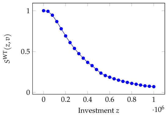
Figure 1.
Impact of the investment z on the Wang transform security breach probability function.
This function possesses the four fundamental properties of the security breach probability models established in Gordon and Loeb (2002) and an additional property described below (see Mazzoccoli and Naldi 2022 for details):
- ;
- ;
- ;
- ;
- .
2.2. Mixed Insurance and Investment in Security Strategy
When combining insurance and investments in the context of cyber risk management, the company incurs two main expenditure terms:
- Investment z: This term represents the amount of money invested in security measures by the company to mitigate cyber risks. These investments aim to reduce the probability of successful attacks and limit potential losses.
- Insurance premium P: The insurance premium is the amount paid by the company to the insurer to obtain insurance coverage. The premium is typically related to the overall policy liability, which in this case corresponds to the potential amount of money that could be lost in the event of a cyber attack.
To determine the insurance premium P, this paper aims to establish a relationship between the premium and the overall potential loss in the event of an attack. The exact estimation method for the loss is not discussed here, but the paper by Eling and Wirfs (2019) provides advancements in this area. The security investments made by the company are expected to reduce the probability of incurring the total potential loss, and consequently, decrease the amount of compensation that would need to be paid by the insurance company.
In summary, the insurance premium takes into account the company’s investments in security, which in turn reduce the probability of incurring a significant loss in the event of a cyber attack. By considering these investments, the premium is adjusted to reflect the reduced potential liability and the expected decrease in the amount of compensation paid by the insurer. Due to its mathematical tractability, in this article, we adopt the expression used by Young et al. (2016); the resulting premium is
where v is again the vulnerability, is the basis premium rate, that is, the premium for the case of full vulnerability () in the absence of investments, and r is the discount rate that modulates how the reduction in vulnerability is transferred to the premium. Naturally, the results obtained in our analysis are constrained by the choice of the insurance premium function and the type of insurance coverage selected (in this case, full loss coverage). In Figure 2, the premium P is represented as a function of the investment z.
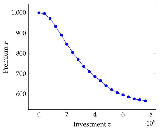
Figure 2.
Trend of the insurance premium as a function of the investment z.
Equation (2) thus represents the premium expression that an insurance company could establish to incentivize self-protection measures taken by its policyholders through a reduction in the premium. This matches with what is stated by Bryce (2001); in fact, numerous insurers provide discounts to customers who utilize managed security service providers or install network security devices, even though the premium is calculated based on the maximum potential amount of damage that the insured can suffer. Therefore, the company’s total expense E is defined as
and, in particular, the insured company aims to minimize this expense.
3. Optimization Problem
In this section, we are approaching a problem that does not admit a closed-form solution for the investment in security z. In particular, we prove the existence of the minimum for the total expense E when insurance and security investments are employed, proving some lemmas and theorems. Then, we explore the validity of the optimal solution, which translates into the company’s decision to invest or not to invest in security. Henceforth, to simplify the notation, we write S instead of .
3.1. Existence of the Optimal Investment Solution
Theorem 1.
The derivative with respect the investment z of the breach probability function is bounded. In particular, the results show that
Proof.
The derivative of the breach probability function with respect the investment z, , is always negative (as described in property ).
In addition,
Furthermore, from the property , there exists an investment so that the second derivative of the breach probability function with respect to the investment z is zero, that is, . In fact, . Consequently, is a minimum for , and .
Since S is a continuous function in , it follows that
□
In Figure 3, the function is represented.
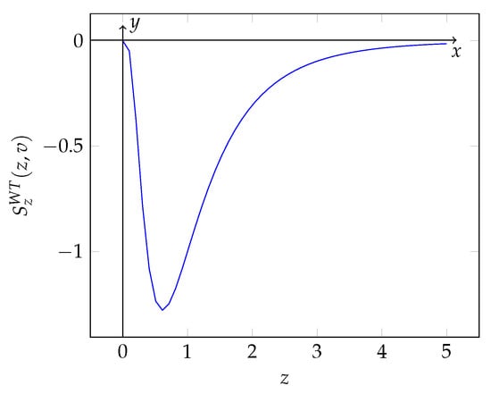
Figure 3.
Trend in the derivative with respect to the investment of the security breach probability function .
Lemma 1.
The derivative of the total expense E with respect to the investment z is bounded. In particular, the results show that
Proof.
The proof of this proposition follows by the previous theorem multiplying by the quantity and then adding 1 to all members of Equation (6)
□
In Figure 4, the function is represented.
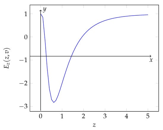
Figure 4.
Trend in the derivative with respect to the investment of the total expense E.
Theorem 2.
The total expense function E has two stationary points and () if and only if the vulnerability is lower than a threshold , where
The two points and are the maximum and minimum for the total expense E, respectively.
Proof.
Let us consider the derivative of the total expense with respect to the investment, . From Equation (5), we obtain that
By the results in Equation (8) and in Lemma 1, the function admits two stationary points and () if and only if is zero for some values of z. This condition is verified if and only if the minimum point of assumes a negative value, or rather
In addition, using again property , since , it follows that the function E is concave for and convex for . Consequently, under the constraint in Equation (9), the stationary point is a maximum point and is a minimum point for the total expense E. □
3.2. Validity of the Optimal Investment Solution
In the previous section, we undertook an examination of the existence of the optimal investment in security solution z. Now, our aim is to delve into the circumstances under which such an investment exists, thereby elucidating when it becomes rational and advantageous for the company to allocate resources toward enhancing its security measures.
In particular, in Equation (9), we have shown that there exists a point of minimum for the company’s total expense E if the vulnerability v does not exceed a certain threshold.
Therefore, a company can decide not to invest in security (that is, it decides to rely completely on the insurance premium) if its vulnerability is over that threshold, that is, . In particular, the decision not to invest for a company can occur in the following circumstances:
- Low insurance premium P;
- Low discount rate r associated with security investments;
- Low effectiveness of security investments ;
- Low probability of an attack t or low loss in the case of a successful attack.
In Figure 5, the region within which the optimal investment in security exists is illustrated, denoted by the highlighted pink area, alongside the contrasting region where it is deemed unsuitable for the company to allocate resources towards security measures, indicated by the highlighted purple area. In particular, the factor exerting the most significant influence on the investment decision is the insurance premium. Moreover, careful analysis reveals that, for a company, the opportunity to invest in security increases as the insurance premium reaches high magnitudes.
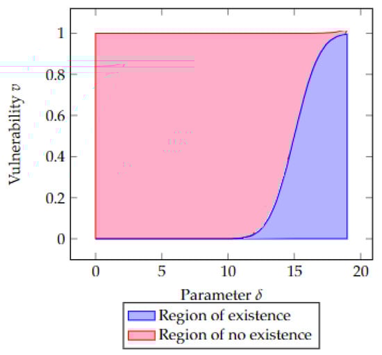
Figure 5.
Region of vulnerability where the optimal investment exists. Parameter values in Table 1 and .
For example, using the expected value principle, it is reasonable to set the premium rate as a fraction of the expected potential loss if any attack is successful, that is, (also known as flat rate pricing), see the paper of Romanosky et al. (2017) or the book of Goovaerts et al. (2001) for details. If we assume the values of the parameters in Table 1, the results show that the threshold is . Therefore, in the considered reference case, a company can decide not to invest in security if its vulnerability is higher than the value of . The parameter values used in Table 1 are derived from statistics and estimates obtained from the scientific literature (see, for example, Gordon and Loeb 2002; Hausken 2006; Young et al. 2016).

Table 1.
Parameter reference case value.
4. Results
In this section, we analyze the effects on the optimal investment in security z by varying the main parameters, the expected loss , the vulnerability v, and the investment effectiveness coefficient . Finally, we also explore the impact of the vulnerability of a firm and the expected loss on the trend of the expenditures in the total expense E. In particular, for this aim, we use values of the parameters in Table 1.
4.1. Optimal Investment as a Function of the Expected Loss
Let us explore the trend of the investment z as a function of the loss . The expected loss is a crucial factor in determining the optimal investment. If the expected loss increases, it generally leads to a higher optimal investment in security. This is because higher expected losses imply a greater potential impact, making it more worthwhile to invest in mitigating the risks.
In Figure 6, we can observe the trend in the optimal investment in security z as a function of the expected loss . In particular, we can see that the optimal investment assumes a different behavior, varying the investment effectiveness coefficient when the expected loss grows. When the coefficient is equal to , the trend in the investment is quite linear; instead, in the other two cases ( and ), it assumes a sublinear fashion. From Figure 6, it is important to underline the role of the investment effectiveness coefficient; variations of this coefficient produce non-linear variations in the optimal investment in security. The interesting thing to note is that if investment efficiency is high, for moderately high loss ratios, there is a preference to invest more in security to obtain a reduced insurance premium. However, for higher expected loss values , if the coefficient of security investment efficiency is not too low, there is a preference to invest more in security to avoid a significant expense required by the insurance premium.
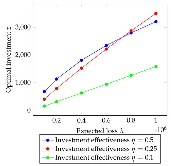
Figure 6.
Optimal investment in security as a function of the expected loss . Parameters values in Table 1.
In both cases, the main objective seems to be balancing security investment with insurance costs. If investment efficiency is high or if the coefficient of security investment efficiency is not too low, there is a preference to invest more in security to gain financial advantages. However, the final choice will depend on a careful assessment of the costs and benefits of both options.
As expected, a too low coefficient indicates greater inefficiency in security investments. Therefore, the company will need to invest more money to achieve the same level of security. The significant inefficiency in security investments leads the company to transfer all the risk of loss to the insurance company.
In this scenario, the company’s lack of investment in security measures results in a higher risk exposure. As a result, they rely heavily on insurance coverage to mitigate potential losses. By transferring the risk to the insurance company, the company hopes to minimize the financial impact in the event of a loss.
4.2. Optimal Investment as a Function of the Vulnerability
Now, we analyze the impact of the vulnerability v on the optimal investment z.
By exploring the optimal investment behavior as the company’s vulnerability varies, we can observe in Figure 7 that for values of investment effectiveness coefficient of 0.1 and 0.25, the optimal investment follows a strictly concave trend, reaching a maximum point. However, for a coefficient value of 0.5, the function is strictly increasing and stops for vulnerability values higher than . This indicates that, for lower values of the coefficient of investment efficiency, it is more beneficial to invest more in security only within a certain range of vulnerability.
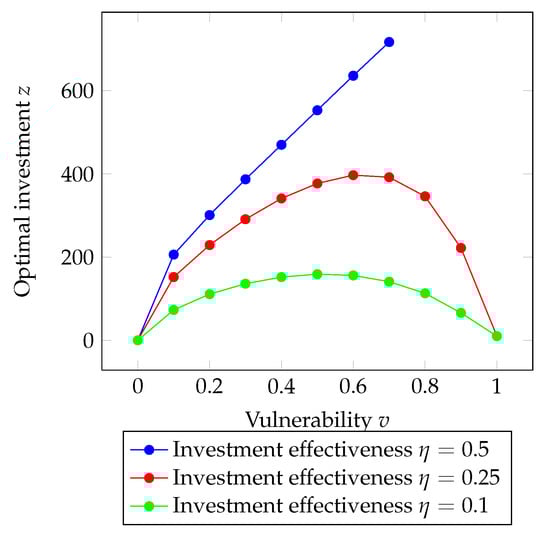
Figure 7.
Optimal investment in security as a function of the vulnerability v. Parameters values in Table 1.
In fact, if the vulnerability is too low, it is not advantageous to invest heavily in security. On the other hand, if the vulnerability is too high, investments would have little effectiveness (thus, opting more for insurance). Conversely, for higher coefficient values, if the vulnerability does not exceed a certain threshold, it is more beneficial to invest more in security since investment efficiency is high. However, if the vulnerability is too high, to avoid excessively high expenses, the reliance on insurance becomes the primary choice.
In summary, the optimal investment in security depends on finding the right balance based on the coefficient of investment efficiency and the vulnerability level. Investments in security should be prioritized within a certain vulnerability range, taking into account the cost-effectiveness and effectiveness of security measures, while also considering the potential expenses associated with relying solely on insurance for high vulnerability levels.
4.3. Total Expense as a Function of the Expected Loss and Vulnerability
By conducting a similar analysis for total expenditure (security investment + insurance premium), it can be observed that the majority of the expenditure is allocated to the insurance premium. In particular, in Figure 8, it can be seen that as the expected loss increases, since the coverage is total, the reliance on insurance increases. However, from the perspective of vulnerability, the scenario is different. It can be observed in Figure 9 that the insurance premium exhibits a very slight increasing variation; on the other hand, security investment increases as vulnerability rises, yet it remains a minority portion (in percentage of total expenditure).
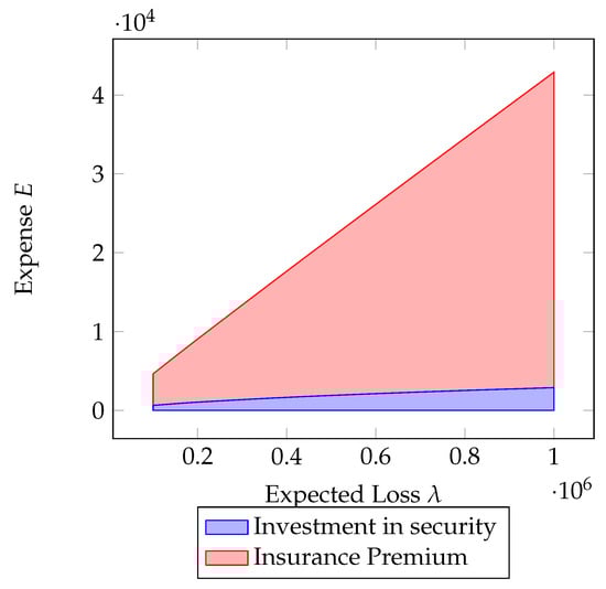
Figure 8.
Impact of the expected loss on the total expense E. Parameter values in Table 1.
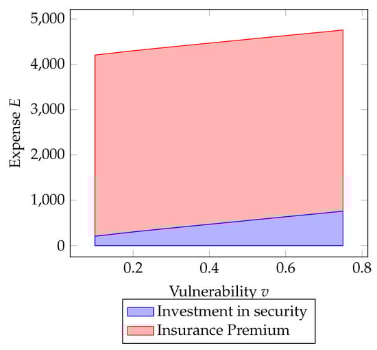
This suggests that as the expected loss grows, the company leans more towards relying on insurance to cover the potential losses. On the other hand, when assessing vulnerability, the company recognizes the importance of investing in security measures to mitigate risks. However, in terms of the overall expenditure, the investment in security, although increasing with vulnerability, remains a smaller proportion compared to the insurance premium.
5. Conclusions
In this paper, we analyzed the optimal investment in cyber security of a firm in a mixed risk management strategy where insurance is employed. Specifically, we used the newest and most innovative security breach probability function to study the problem of optimizing investment in cyber security for a company in order to mitigate cyber risk. In addition, to prove the existence of a minimum point for overall expenditure composed of investments in security and insurance premiums against economic damages caused by cyber attacks, we analyzed the mathematical properties of the total expense (composed of investment in security and insurance premium). For this type of analysis, we have taken into account the company’s vulnerability, the efficiency of security investments, the probabilities of attacks by hackers, and the insurance premium mitigated by security investments. Consequently, we explored the trend in optimal expense in security based on the most important parameters: expected loss, vulnerability, and investment coefficient. In particular, in the case of full loss coverage, we inferred that the majority of investments are aimed toward insurance premium. This is mainly due to the fact that total coverage of losses caused by cyber attacks discourages companies, to some extent, from investing in cyber security. In future research, we will investigate security investments when insurance coverage is partial or includes deductibles. Taking a comprehensive view of insurance options for coverage, we will analyze which parameters have the most significant impact on the sensitivity of the optimal security investment.
Funding
This research received no external funding.
Data Availability Statement
Not applicable.
Conflicts of Interest
The authors declare no conflict of interest.
References
- Allodi, Luca, and Fabio Massacci. 2017. Security events and vulnerability data for cybersecurity risk estimation. Risk Analysis 37: 1606–27. [Google Scholar] [CrossRef] [PubMed]
- Anderson, Ross, Chris Barton, Rainer Böhme, Richard Clayton, Michel J. G. Van Eeten, Michael Levi, Tyler Moore, and Stefan Savage. 2013. Measuring the cost of cybercrime. In The Economics of Information Security and Privacy. Berlin and Heidelberg: Springer, pp. 265–300. [Google Scholar]
- Arcuri, Maria Cristina, Marina Brogi, and Gino Gandolfi. 2017. How does cyber crime affect firms? The effect of information security breaches on stock returns. Paper presented at First Italian Conference on Cybersecurity (ITASEC17), Venice, Italy, January 17–20; pp. 175–93. [Google Scholar]
- Aven, Terje. 2011. Quantitative Risk Assessment: The Scientific Platform. Cambridge: Cambridge University Press. [Google Scholar]
- Aven, Terje, and Roger Flage. 2020. Foundational challenges for advancing the field and discipline of risk analysis. Risk Analysis 40: 2128–36. [Google Scholar] [CrossRef] [PubMed]
- Bojanc, Rok, and Borka Jerman-Blažič. 2008. An economic modelling approach to information security risk management. International Journal of Information Management 28: 413–22. [Google Scholar] [CrossRef]
- Bryce, Robert. 2001. Hack Insurer Adds Microsoft Surcharge. Interactive Week, August 22. [Google Scholar]
- Cashell, Brian, William D. Jackson, Mark Jickling, and Baird Webel. 2004. The Economic Impact of Cyber-Attacks. Congressional Research Service Documents, CRS RL32331. Washington, DC: Government and Finance Division, p. 2. [Google Scholar]
- Chong, Wing Fung, Runhuan Feng, Hins Hu, and Linfeng Zhang. 2022. Cyber Risk Assessment for Capital Management. arXiv. [Google Scholar] [CrossRef]
- Dieye, Rokhaya, Ahmed Bounfour, Altay Ozaygen, and Niaz Kammoun. 2020. Estimates of the macroeconomic costs of cyber-attacks. Risk Management and Insurance Review 2: 183–208. [Google Scholar] [CrossRef]
- Eling, Martin, and Jan Wirfs. 2019. What are the actual costs of cyber risk events? European Journal of Operational Research 272: 1109–19. [Google Scholar] [CrossRef]
- Feng, Shaohan, Zehui Xiong, Dusit Niyato, Ping Wang, Shaun Shuxun Wang, and Xuemin Sherman Shen. 2020. Joint pricing and security investment in cloud security service market with user interdependency. IEEE Transactions on Services Computing 15: 1461–72. [Google Scholar] [CrossRef]
- Franke, Ulrik. 2017. The cyber insurance market in Sweden. Computers & Security 68: 130–44. [Google Scholar]
- Furnell, Steven, Harry Heyburn, Andrew Whitehead, and Jayesh Navin Shah. 2020. Understanding the full cost of cyber security breaches. Computer Fraud & Security 12: 6–12. [Google Scholar]
- Ghelani, Diptiben. 2022. Cyber security, cyber threats, implications and future perspectives: A Review. Authorea Preprints, September 22, 1461–72. [Google Scholar]
- Goovaerts, Marc, Rob Kaas, Jan Dhaene, and Michel Denuit. 2001. Modern Actuarial Risk Theory. Dordrecht: Kluwer Academic. [Google Scholar]
- Gordon, Lawrence A., and Martin P. Loeb. 2002. The economics of information security investment. ACM Transactions on Information and System Security (TISSEC) 5: 438–57. [Google Scholar] [CrossRef]
- Hausken, Kjell. 2006. Returns to information security investment: The effect of alternative information security breach functions on optimal investment and sensitivity to vulnerability. Information Systems Frontiers 8: 338–49. [Google Scholar] [CrossRef]
- Hovav, Anat, and John D’Arcy. 2003. The impact of denial-of-service attack announcements on the market value of firms. Risk Management and Insurance Review 6: 97–121. [Google Scholar] [CrossRef]
- Kaas, Rob, Marc Goovaerts, Jan Dhaene, and Michel Denuit. 2008. Modern Actuarial Risk Theory: Using R. Berlin and Heidelberg: Springer Science & Business Media, vol. 128. [Google Scholar]
- Kamiya, Shinichi, Jun-Koo Kang, Jungmin Kim, Andreas Milidonis, and René M. Stulz. 2020. Risk management, firm reputation, and the impact of successful cyberattacks on target firms. Journal of Financial Economics 139: 719–49. [Google Scholar] [CrossRef]
- Khalili, Mohammad Mahdi, Parinaz Naghizadeh, and Mingyan Liu. 2018. Designing cyber insurance policies: The role of pre-screening and security interdependence. IEEE Transactions on Information Forensics and Security 13: 2226–39. [Google Scholar] [CrossRef]
- Krutilla, Kerry, Alexander Alexeev, Eric Jardine, and David Good. 2021. The benefits and costs of cybersecurity risk reduction: A dynamic extension of the Gordon and Loeb model. Risk Analysis 41: 1795–808. [Google Scholar] [CrossRef]
- Lallie, Harjinder Singh, Lynsay A. Shepherd, Jason R. C. Nurse, Arnau Erola, Gregory Epiphaniou, Carsten Maple, and Xavier Bellekens. 2021. Cyber security in the age of COVID-19: A timeline and analysis of cyber-crime and cyber-attacks during the pandemic. Computers & Security 105: 102248. [Google Scholar]
- Maillart, Thomas, and Didier Sornette. 2010. Heavy-tailed distribution of cyber-risks. The European Physical Journal B 75: 357–64. [Google Scholar] [CrossRef]
- Marotta, Angelica, Fabio Martinelli, Stefano Nanni, Albina Orlando, and Artsiom Yautsiukhin. 2017. Cyber-insurance survey. Computer Science Review 24: 35–61. [Google Scholar] [CrossRef]
- Mastroeni, Loretta, Alessandro Mazzoccoli, and Maurizio Naldi. 2019. Service level agreement violations in cloud storage: Insurance and compensation sustainability. Future Internet 11: 142. [Google Scholar] [CrossRef]
- Mayadunne, Sanjaya, and Sungjune Park. 2016. An economic model to evaluate information security investment of risk-taking small and medium enterprises. International Journal of Production Economics 182: 519–30. [Google Scholar] [CrossRef]
- Mazzoccoli, Alessandro, and Maurizio Naldi. 2020a. Robustness of optimal investment decisions in mixed insurance/investment cyber risk management. Risk Analysis 30: 550–64. [Google Scholar] [CrossRef] [PubMed]
- Mazzoccoli, Alessandro, and Maurizio Naldi. 2020b. The expected utility insurance premium principle with fourth-order statistics: Does it make a difference? Algorithms 13: 116. [Google Scholar] [CrossRef]
- Mazzoccoli, Alessandro, and Maurizio Naldi. 2021. Optimal investment in cyber-security under cyber insurance for a multi-branch firm. Risks 9: 24. [Google Scholar] [CrossRef]
- Mazzoccoli, Alessandro, and Maurizio Naldi. 2022. An Overview of Security Breach Probability Models. Risks 10: 220. [Google Scholar] [CrossRef]
- Meland, Per Hakon, Inger Anne Tondel, and Bjornar Solhaug. 2015. Mitigating risk with cyberinsurance. IEEE Security & Privacy 13: 38–43. [Google Scholar]
- Mukhopadhyay, Arunabha, Samir Chatterjee, Kallol K. Bagchi, Peteer J. Kirs, and Girja K. Shukla. 2019. Cyber risk assessment and mitigation (cram) framework using logit and probit models for cyber insurance. Information Systems Frontiers 21: 997–1018. [Google Scholar] [CrossRef]
- Murphy, Diane R., and Richard H. Murphy. 2013. Teaching cybersecurity: Protecting the business environment. Paper presented at 2013 on InfoSecCD’13: Information Security Curriculum Development Conference, Kennesaw, GA, USA, October 12; pp. 88–93. [Google Scholar]
- Naldi, Maurizio, and Alessandro Mazzoccoli. 2018. Computation of the insurance premium for cloud services based on fourth-order statistics. International Journal of Simulation: Systems, Science and Technology 19: 1–6. [Google Scholar] [CrossRef]
- Naldi, Maurizio, Marta Flamini, and Giuseppe D’Acquisto. 2018. Negligence and sanctions in information security investments in a cloud environment. Electronic Markets 28: 39–52. [Google Scholar] [CrossRef]
- Palsson, Kjartan, Steinn Gudmundsson, and Sachin Shetty. 2020. Analysis of the impact of cyber events for cyber insurance. The Geneva Papers on Risk and Insurance-Issues and Practice 45: 564–79. [Google Scholar] [CrossRef]
- Paté-Cornell, M.-Elisabeth, Marshall Kuypers, Matthew Smith, and Philip Keller. 2018. Cyber risk management for critical infrastructure: A risk analysis model and three case studies. Risk Analysis 38: 226–41. [Google Scholar] [CrossRef]
- Peterson, Kevin. 2020. What Is Risk Management? In The Professional Protection Officer. Amsterdam: Elsevier, pp. 367–72. [Google Scholar]
- Pollmeier, Santiago, Ivano Bongiovanni, and Sergeja Slapničar. 2023. Designing a financial quantification model for cyber risk: A case study in a bank. Safety Science 159: 106022. [Google Scholar] [CrossRef]
- Poufinas, Thomas, and Nikolaos Vordonis. 2018. Pricing the cost of cybercrime—A financial protection approach. iBusiness 10: 128. [Google Scholar] [CrossRef]
- Refsdal, Atle, Bjørnar Solhaug, and Ketil Stølen. 2015. Cyber-Risk Management. New York: Springer, pp. 33–47. [Google Scholar]
- Romanosky, Sasha. 2016. Examining the costs and causes of cyber incidents. Journal of Cybersecurity 2: 121–35. [Google Scholar] [CrossRef]
- Romanosky, Sasha, Lilian Ablon, Andreas Kuehn, and Therese Jones. 2017. Content Analysis of Cyber Insurance Policies: How Do Carriers Write Policies and Price Cyber Risk? Available online: https://papers.ssrn.com/sol3/papers.cfm?abstract_id=2929137 (accessed on 3 April 2023).
- Rosson, Jack, Mason Rice, Juan Lopez, and David Fass. 2019. Incentivizing cyber security investment in the power sector using an extended cyber insurance framework. Homeland Security Affairs 15: 1–25. [Google Scholar]
- Scala, Natalie M., Allison C. Reilly, Paul L. Goethals, and Michel Cukier. 2019. Risk and the five hard problems of cybersecurity. Risk Analysis 39: 2119–26. [Google Scholar] [CrossRef] [PubMed]
- Smith, Zhanna Malekos, and Eugenia Lostri. 2020. The Hidden Costs of Cybercrime. Technical Report. San Jose: Center for Strategic and International Studies. [Google Scholar]
- Strupczewski, Grzegorz. 2018. Current state of the cyber insurance market. Paper presented at 10th Economics and Finance Conference, Rome, Italy, September 10–13; Number 6910062. Rome: International Institute of Social and Economic Sciences. [Google Scholar]
- Taherdoost, Hamed. 2022. Understanding cybersecurity frameworks and information security standards—A review and comprehensive overview. Electronics 11: 2181. [Google Scholar] [CrossRef]
- The Ponemon Institute. 2016. 2016 Cost of Data Breach Study: Global Analysis. Technical Report. Traverse City: The Ponemon Institute. [Google Scholar]
- Venkatachary, Sampath Kumar, Jagdish Prasad, and Ravi Samikannu. 2017. Economic impacts of cyber security in energy sector: A review. International Journal of Energy Economics and Policy, EconJournals 7: 130–44. [Google Scholar]
- Wang, Shaun. 2017. Optimal Level and Allocation of Cybersecurity Spending: Model and Formula. SSRN Preprint No. 3010029. Available online: https://papers.ssrn.com/sol3/papers.cfm?abstract_id=3010029 (accessed on 16 November 2022).
- Wang, Shaun S. 2019. Integrated framework for information security investment and cyber insurance. Pacific-Basin Finance Journal 57: 101173. [Google Scholar] [CrossRef]
- Wheatley, Spencer, Thomas Maillart, and Didier Sornette. 2016. The extreme risk of personal data breaches and the erosion of privacy. The European Physical Journal B 89: 1–12. [Google Scholar] [CrossRef]
- Wu, Yong, Gengzhong Feng, Nengmin Wang, and Huigang Liang. 2015. Game of information security investment: Impact of attack types and network vulnerability. Expert Systems with Applications 42: 6132–46. [Google Scholar] [CrossRef]
- Xu, Lu, Yanhui Li, and Jing Fu. 2019. Cybersecurity investment allocation for a multi-branch firm: Modeling and optimization. Mathematics 7: 587. [Google Scholar] [CrossRef]
- Xu, Maochao, Kristin M. Schweitzer, Raymond M. Bateman, and Shouhuai Xu. 2018. Modeling and predicting cyber hacking breaches. IEEE Transactions on Information Forensics and Security 13: 2856–71. [Google Scholar] [CrossRef]
- Young, Derek, Juan Lopez, Mason Rice, Benjamin Ramsey, and Robert McTasney. 2016. A framework for incorporating insurance in critical infrastructure cyber risk strategies. International Journal of Critical Infrastructure Protection 14: 43–57. [Google Scholar] [CrossRef]


Disclaimer/Publisher’s Note: The statements, opinions and data contained in all publications are solely those of the individual author(s) and contributor(s) and not of MDPI and/or the editor(s). MDPI and/or the editor(s) disclaim responsibility for any injury to people or property resulting from any ideas, methods, instructions or products referred to in the content. |
© 2023 by the author. Licensee MDPI, Basel, Switzerland. This article is an open access article distributed under the terms and conditions of the Creative Commons Attribution (CC BY) license (https://creativecommons.org/licenses/by/4.0/).