Asymptotic Methods for Transaction Costs

Abstract

We propose a general approximation method for the determination of optimal trading strategies in markets with proportional transaction costs, with a polynomial approximation of the residual value function. The method is exemplified by several problems, from optimally tracking benchmarks and hedging the log contract to maximizing utility from terminal wealth. Strategies are also approximated by practically executable, discrete trades. We identify the necessary trade-off between the trading frequency and trade size to ensure satisfactory agreement with the theoretically optimal, continuous strategies of infinite activity.

1. Introduction

It was explained to me that the effects on which one was working were so vanishingly small that without the greatest possible precision in computation they might have been missed altogether.

Norbert Wiener1

Optimal trading strategies in a Black–Scholes market or its extensions face challenges when applied to realistic markets with friction, including transaction costs, price impacts, or margin requirements. For instance, employing a constant proportion trading strategy or a standard Delta hedge in the Black–Scholes model becomes practically infeasible in the presence of a relative bid–ask spread $\epsilon$, as it may lead to immediate bankruptcy due to trading policies of infinite variation. In order to maintain solvency in markets with proportional transaction costs, the trading frequency is adjusted to finite variation, involving the minimal trades necessary to stay close to the target exposures. The deviation from this target exposure is of order ${\epsilon }^{1/3}$, while the impact on the transaction costs is of the second order (that is, of magnitude ${\epsilon }^{2/3}$, cf. Shreve and Soner (1994); Gerhold et al. (2014); Kallsen and Muhle-Karbe (2017); Rogers (2004)). Determining long-run optimal trading strategies or solutions to infinite horizon problems involves solving specific free boundary problems. These problems define the boundaries that limit the maximum deviation of a portfolio statistic ${\xi }_t$ from the target, where these statistics commonly represent the proportion of wealth in the risky asset, the risky–safe ratio, or transformed variants. For constant investment opportunities, an investor refrains from trading when ${\xi }_t$ is outside a constant region $[{\xi }_{-},{\xi }_{+}]$, engaging in minimal trading only at the boundaries ${\xi }_{\pm }$ to maintain the statistic within the interval. This strategy is embodied by a diffusion with two reflecting boundaries and is referred to as a control limit policy Taksar et al. (1988). The parameterization of the involved equations and the methods to solve them are customized for each specific setup. However, the analytical methods are highly technical, making them suitable for an expert audience. Moreover, the resulting optimal trading policies are reflected diffusions (cf. Tanaka (1979)), making them impractical for implementation as they entail infinite activity.

The aim of this paper is to address these challenges by introducing asymptotic methods, both for the approximation of the value functions in various problems and the design of asymptotically optimal trading policies that can be executed in real trading environments. Asymptotic methods have proved instrumental in understanding the sensitivity of trading boundaries and welfare to different market and risk aversion parameters (cf. the ingenious insights of Constantinides (1986) based on numerical computation, with the financial interpretation of the asymptotic expansions derived in Kallsen and Muhle-Karbe (2017); Gerhold et al. (2012, 2014).

First, we employ finite activity strategies to approximate control limit policies. In contrast to reflected diffusions, these strategies can be implemented in a real trading environment. They involve trades of fixed size aimed at re-aligning a portfolio statistic with its frictionless target, such as adjusting the proportion of wealth ${\pi }_t$ in the risky asset when reaching ${\pi }_{\pm }$. Acknowledging the insightful contribution of Shreve and Soner (1994, Appendix B), which highlights that no-trade regions typically scale with a size proportional to ${\epsilon }^{1/3}$, discrete trades in this context must be of the same or higher order as the bid–ask spread. The findings of this paper offer an alternative answer to the question of Rogers (2004) regarding the ${\epsilon }^{2/3}$ effect of proportional transaction costs on welfare. Approximating the control limit policy with trades of fixed size reveals that the transaction costs, at the leading order, are a product of the bid–ask spread ($\epsilon$), trade size (${\epsilon }^{\alpha /3}$ for $\alpha \ge 1$), and trading frequency (proportional to ${\epsilon }^{-\frac{1}{3}(\alpha +1)}$), resulting in the same cost of order ${\epsilon }^{2/3}$, irrespective of the smallness of the trades (dictated by the parameter $\alpha$) or the objective under consideration.

Second, we put forward a general approximation method for pertinent free boundary problems, which often2 can be expressed as

$$\begin{array}{cc}\hfill & F(g,g^{\prime },g^{″})=0,\hfill \end{array}$$

(1)

$$\begin{array}{cc}\hfill g\left({\pi }_{-}\right)& =1,g\left({\pi }_{+}\right)=1-\epsilon ,\hfill \end{array}$$

(2)

$$\begin{array}{cc}\hfill g^{\prime }\left({\pi }_{-}\right)& =0,g^{\prime }\left({\pi }_{+}\right)=0.\hfill \end{array}$$

(3)

Here, an unknown scalar $g=g\left(\pi \right)$ representing the proportion of wealth $\pi$ in the risky asset is involved. The function g must satisfy a second-order ODE (1) between the buy and sell boundaries ${\pi }_{-}$ and ${\pi }_{+}$ and boundary conditions (2) and (3). While the latter are universal, the ODE (1) identifies the specific objective under consideration. The approximation method relies on a polynomial expansion of the scalar function g and an asymptotic Ansatz for the trading boundaries ${\pi }_{\pm }$.

The parameter $\epsilon$ in the condition (2) represents the relative bid–ask spread of the risky asset S, where one purchases the asset at time t at the ask price $S_t$ and sells it at the slightly lower price $(1-\epsilon )S_t$ (ibid). This boundary condition’s specific form lends itself to the financial interpretation of a frictionless price $\tilde{S}$ with a functional form expressed as ${\tilde{S}}_t:=g\left({\pi }_t\right)S_t$. This serves as a potential shadow price, which is a fictitious risky asset evolving within the bid–ask spread $S_t(1-\epsilon )\le {\tilde{S}}_t\le S_t$ and which aligns precisely with the bid or ask of S whenever the optimal strategy for $\tilde{S}$ involves executing trades. This asset is indeed a shadow price for power and log-utility, as noted in previous studies by Gerhold et al. (2013, 2014); Guasoni and Muhle-Karbe (2013). However, for certain local criteria, it might only serve as an asymptotic shadow price (or none at all), as discussed in Kallsen and Muhle-Karbe (2017); Mayerhofer (2024). Notwithstanding this issue, our method is applicable for equations both in the original markets and in potential shadow markets. A distinctive aspect of this paper lies in its examination of Neuberger’s log contract Neuberger (1994) and its dynamic hedge under proportional transaction costs, supplementing the well-explored objectives with known solutions in the literature. Due to the straightforward form of its free boundary problem, our analysis may serve as a valuable introductory example for graduate students delving into the realm of optimization under proportional transaction costs.

Program of Paper

The paper’s structure is organized as follows. Section 2 introduces the market model, encompassing a risky Black–Scholes asset with transaction costs, along with the presentation of relevant admissible strategies for this study. Section 3 comprises three distinct parts.

Section 3.1 investigates three strategies and evaluates their performance in terms of the trading frequency and long-run cost. This includes the examination of minimal trades (control limit policies; see Section 3.1.1), maximal trades (discrete trades directly to the target; see Section 3.1.2), and small trades (sufficiently small trades to closely align with control limit policies; see Section 3.1.3). Section 3.2 is dedicated to optimization problems related to tracking specific targets. It includes the computation of asymptotic approximations for the free boundary problem for leveraged ETFs (see Section 3.2.1) and optimally hedging a log contract (see Section 3.2.4). Section 3.3 examines classical objectives with a long-run horizon, featuring the risk-averse investor (Section 3.3.1), the log-utility investor (Section 3.3.2), and the risk-neutral investor (Section 3.3.3). The interpretation and discussion of these results are presented in Section 4.

2. Materials and Methods

In our financial market model, there are two tradable assets: a risk-free asset with continuous compounding at a rate $r\ge 0$ and a risky asset S with ask price $S_t$, governed by the dynamics

$$\frac{d{S}_t}{S_t}=(\mu +r)dt+\sigma d{B}_t,S_0,\sigma >0,\mu \ge 0,$$

(4)

where B denotes a standard Brownian motion. We introduce a relative bid–ask spread $\epsilon >0$, ensuring that the risky asset is sold at $(1-\epsilon )S_t$.

In markets with friction, the trading strategies need to be modified so as to ensure solvency. In the presence of transaction costs, solvency constraints dictate that only finite-variation trading strategies are viable.3 Let $X_t$ be the safe position and $Y_t$ the risky position. Furthermore, denote by ${\left({\phi }_t^{\uparrow }\right)}_{t\ge 0}$ and ${\left({\phi }_t^{\downarrow }\right)}_{t\ge 0}$ the cumulative number of shares bought and sold, respectively. The total wealth, assessed at the ask, is given by $w_t=X_t+Y_t=X_t+{\phi }_t{S}_t$, where ${\phi }_t={\phi }_t^{\uparrow }-{\phi }_t^{\downarrow }$.

In this paper, we study two types of trading strategies. For continuous ${\phi }_t$, the self-financing condition reads

$$\begin{array}{cc}\hfill X_t& =X_0+{\int }_0^{t}r{X}_{u}du-{\int }_0^t{S}_{u}d{\phi }_u^{\uparrow }+(1-\epsilon ){\int }_0^t{S}_{u}d{\phi }_u^{\downarrow },\hfill \\ \hfill Y_t& =Y_0+{\int }_0^t{S}_{u}d{\phi }_u^{\uparrow }-{\int }_0^t{S}_{u}d{\phi }_u^{\downarrow }+{\int }_0^t{\phi }_{u}d{S}_u.\hfill \end{array}$$

(5)

If ${\phi }_t$ is a finite activity jumps process of the pure jump type, such that

$${\phi }_t^{\uparrow }=\sum _{s\le t}\Delta {\phi }_s^{\uparrow },{\phi }_t^{\downarrow }=\sum _{s\le t}\Delta {\phi }_s^{\downarrow },$$

then the self-financing condition reads

$$\begin{array}{cc}\hfill X_t& =X_0+{\int }_0^{t}r{X}_{u}du-\sum _{u\le t}{S}_u\Delta {\phi }_t^{\uparrow }+(1-\epsilon )\sum _{u\le t}{S}_u\Delta {\phi }_u^{\downarrow },\hfill \\ \hfill Y_t& =Y_0+\sum _{u\le t}{S}_u\Delta {\phi }_u^{\uparrow }-\sum _{u\le t}{S}_u\Delta {\phi }_u^{\downarrow }+{\int }_0^t{\phi }_{u_{-}}d{S}_u.\hfill \end{array}$$

(6)

The following defines admissible strategies.

Definition 1.

The trading policy $(x=X_0+{\phi }_0{Y}_0,{\phi }_t={\phi }_t^{\uparrow }-{\phi }_t^{\downarrow })$ is admissible if

(i) 

${\left({\phi }_t^{\uparrow }\right)}_{t\ge 0}$ and ${\left({\phi }_t^{\downarrow }\right)}_{t\ge 0}$ are right-continuous, increasing, and non-anticipating processes;

(ii) 

It is self-financing, satisfying (5) resp. (6).

The collection of admissible trading policies is denoted by Φ.

Depending on the specific optimization criterion, some extra integrability or solvency conditions may apply. (Since we focus on asymptotic methods to solve a range of free boundary problems, we refrain from formulating them explicitly.)

The next statement elaborates the dynamics of wealth, its fraction in the risky asset, and the ratio of risky and safe investment.

Lemma 1.

For any admissible, continuous trading strategy φ, we have

$$\begin{array}{cc}\hfill \frac{d{\zeta }_t}{{\zeta }_t}& =\mu dt+\sigma d{B}_t+(1+{\zeta }_t)\frac{d{\phi }_t^{\uparrow }}{{\phi }_t}-(1+(1-\epsilon ){\zeta }_t)\frac{d{\phi }_t^{\downarrow }}{{\phi }_t},\hfill \\ \hfill \frac{d{w}_t}{w_t}& =rdt+{\pi }_t(\mu dt+\sigma d{B}_t-\epsilon \frac{d{\phi }_t^{\downarrow }}{{\phi }_t}),\hfill \\ \hfill \frac{d{\pi }_t}{{\pi }_t}& =(1-{\pi }_t)(\mu dt+\sigma d{B}_t)-{\pi }_t(1-{\pi }_t){\sigma }^{2}dt+\frac{d{\phi }_t^{\uparrow }}{{\phi }_t}-(1-\epsilon {\pi }_t)\frac{d{\phi }_t^{\downarrow }}{{\phi }_t}.\hfill \end{array}$$

(7)

If ${\phi }_t$ is of the pure jump type (cf. (6)), the same statistics satisfy similar equations, perhaps most rigorously stated in integral form:

$$\begin{array}{cc}\hfill {\zeta }_t& ={\zeta }_0+{\int }_0^t{\zeta }_{s_{-}}\left(\mu ds+\sigma d{B}_s\right)+\sum _{s\le t}{\zeta }_{s_{-}}(1+{\zeta }_{s_{-}})\frac{\Delta {\phi }_s^{\uparrow }}{{\phi }_{s_{-}}}\hfill \\ \hfill & -\sum _{s\le t}{\zeta }_{s_{-}}(1+(1-\epsilon ){\zeta }_{s_{-}})\frac{\Delta {\phi }_s^{\downarrow }}{{\phi }_{s_{-}}},\hfill \\ \hfill w_t& =w_0+r{\int }_0^t{w}_{s_{-}}ds+{\int }_0^t{w}_{s_{-}}{\pi }_{s_{-}}(\mu ds+\sigma d{B}_s)-\sum _{s\le t}\epsilon w_{s_{-}}\frac{\Delta {\phi }_s^{\downarrow }}{{\phi }_{s_{-}}},\hfill \\ \hfill {\pi }_t& ={\pi }_0+{\int }_0^t{\pi }_{s_{-}}(1-{\pi }_{s_{-}})(\mu ds+\sigma d{B}_s)-{\int }_0^t{\pi }_{s_{-}}^2(1-{\pi }_{s_{-}}){\sigma }^{2}ds\hfill \\ \hfill & +\sum _{s\le t}{\pi }_{s_{-}}\frac{\Delta {\phi }_s^{\uparrow }}{{\phi }_{s_{-}}}-\sum _{s\le t}{\pi }_{s_{-}}(1-\epsilon {\pi }_{s_{-}})\frac{\Delta {\phi }_s^{\downarrow }}{{\phi }_{s_{-}}}.\hfill \end{array}$$

(8)

Proof. 

The dynamics (7) are stated and proven in (Guasoni and Mayerhofer 2019, Lemma A.2), which can be adapted for discrete trades, so as to obtain (8). □

3. Results

3.1. Transaction Cost Asymptotics

Reflected diffusions are continuous processes and of finite variation by construction; therefore, strategies of this kind are admissible in the presence of proportional transaction costs. While optimal across a range of optimization criteria in theory, they are practically unrealized due to actual trades occurring discretely in time. In this section, we approximate continuous trading policies with those that trade fixed amounts of the risky asset, thus introducing jumps. The primary challenge lies in quantifying the minimal trade size required to achieve nearly optimal performance. While larger trades align better with a target, they also incur greater costs (cf. Figure 1).

In this section, we investigate the transaction costs and trading frequency associated with three strategies aimed at maintaining a portfolio statistic near a target. These strategies include the following.

(i)

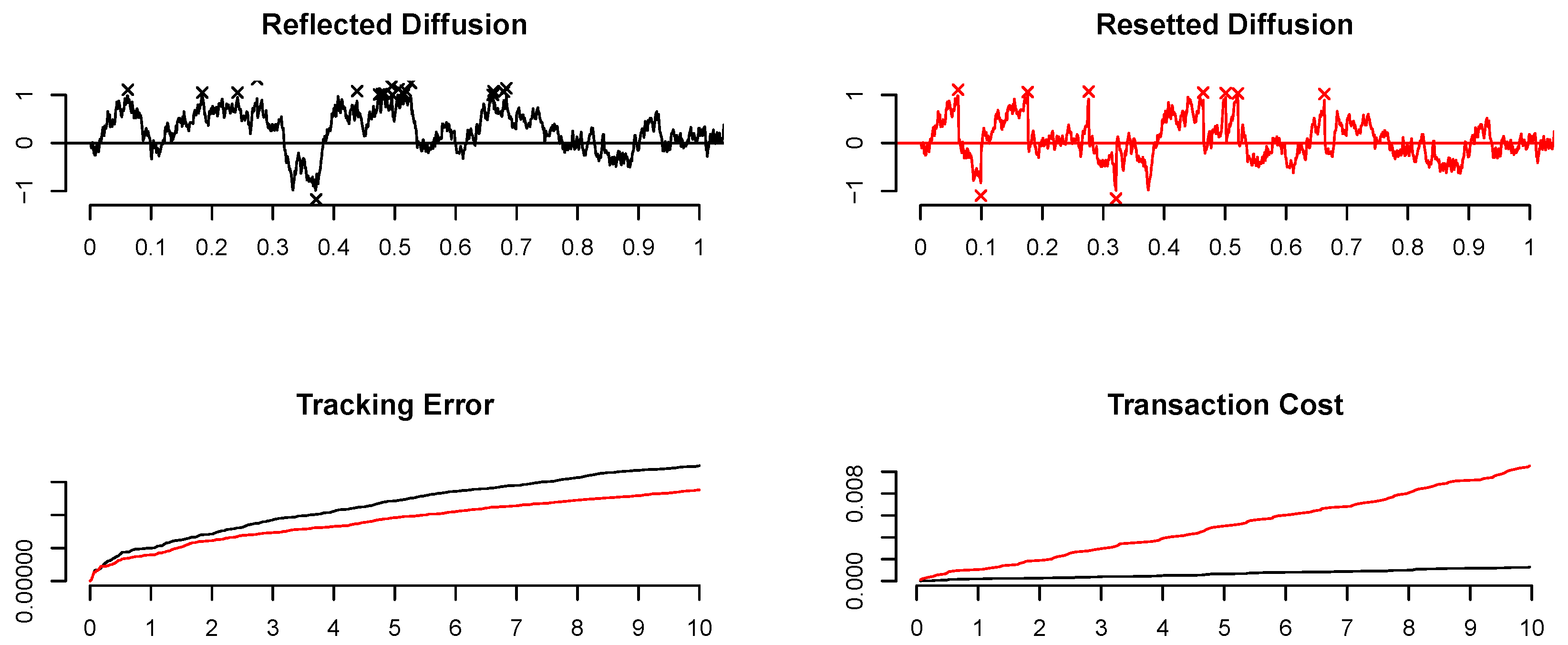
Minimal trades: These strategies operate continuously, engaging in minimal trading at the boundaries of specific no-trade regions (cf. the first plot of Figure 1 (black lines)).

(ii)

Maximal trades: These strategies reset a portfolio statistic to its target value once it reaches these boundaries (cf. the first second plot in Figure 1 (red lines)).

(iii)

Small trades: These involve smaller trades than (ii) made in the direction of the target value.

The general framework involves a geometric Brownian motion $\xi$ with a drift parameter M and diffusion parameter $\Sigma$ evolving in an interval $[{\xi }_{-},{\xi }_{+}]$, reflected at its boundaries ${\xi }_{\pm }$. The financial interpretation of $\xi$ varies among examples, representing either the risky–safe ratio ${\zeta }_t$ or the risky position $Y_t$. Similarly, the processes that confine the GBM within $[{\xi }_{-},{\xi }_{+}]$ vary, influencing the definition of the transaction costs.

Each subsection begins by outlining this general setup of a reflected or resetted geometric Brownian motion. We introduce two types of transaction costs: the average transaction costs (ATC), measuring the negative contribution to infinitesimal returns due to a non-zero bid–ask spread, and the transaction costs (TRC), which quantify the actual long-term cost per time unit. The ATC arises for leveraged ETFs in Section 3.2.1 and for the risk-neutral investor in Section 3.3.3 as a penalty in the objective4, whereas the TRC provides the penalty for the log contract in Section 3.2.4.

3.1.1. Minimal Trades

The dynamics of a reflected GBM are

$$d{\xi }_t={\xi }_t\left(Mdt+\Sigma d{W}_t+d{L}_t-d{U}_t\right),$$

(9)

where L resp. U are local times, with the only points of increase (resp. decrease) on ${\xi }_t={\xi }_{-}$ (resp. ${\xi }_t={\xi }_{+}$).

We shall need the stationary density of a reflected diffusion (Guasoni and Mayerhofer 2019, Lemma B.5).

Lemma 2.

Let ${\xi }_{-}<{\xi }_{+}$. Then, there exists an admissible trading strategy $\widehat{\phi }$ such that the risky–safe ratio ${\xi }_t$ satisfies SDE (7). Moreover, $({\xi }_t,{\widehat{\phi }}_t^{\uparrow },{\widehat{\phi }}_t^{\downarrow })$ is a reflected diffusion on the interval $[{\xi }_{-},{\xi }_{+}]$. In particular, if ${\xi }_{-}>0$, then ${\xi }_t$ has stationary density that equals

$$\nu \left(\xi \right):=\frac{\frac{2\mu }{{\sigma }^2}-1}{{\xi }_{+}^{\frac{2\mu }{{\sigma }^2}-1}-{\xi }_{-}^{\frac{2\mu }{{\sigma }^2}-1}}{\xi }^{\frac{2\mu }{{\sigma }^2}-2},\xi \in [{\xi }_{-},{\xi }_{+}],$$

and, if ${\xi }_{+}<-1$, then

$$\nu \left(\xi \right):=\frac{\frac{2\mu }{{\sigma }^2}-1}{|{\xi }_{-}{|}^{\frac{2\mu }{{\sigma }^2}-1}-{\left|{\xi }_{+}\right|}^{\frac{2\mu }{{\sigma }^2}-1}}{\left|\xi \right|}^{\frac{2\mu }{{\sigma }^2}-2},\xi \in [{\xi }_{-},{\xi }_{+}].$$

The trading strategy in Lemma 2 is called the “control limit policy”, cf. Taksar et al. (1988); Mayerhofer (2024).

We start with the following.

Lemma 3.

$$\begin{array}{cc}\hfill L_{\infty }& :=\underset{T\to \infty }{lim}\frac{1}{T}{\int }_0^{T}d{L}_t=\underset{T\to \infty }{lim}\frac{1}{T}{L}_t=\frac{{\Sigma }^2}{2}\frac{2M/{\Sigma }^2-1}{\left({({\xi }_{+}/{\xi }_{-})}^{2M/{\Sigma }^2-1}-1\right)},\hfill \end{array}$$

(10)

$$\begin{array}{cc}\hfill U_{\infty }& :=\underset{T\to \infty }{lim}\frac{1}{T}{U}_t=\frac{{\Sigma }^2}{2}\frac{1-2M/{\Sigma }^2}{\left({({\xi }_{+}/{\xi }_{-})}^{1-2M/{\Sigma }^2}-1\right)}.\hfill \end{array}$$

(11)

Proof. 

(cf. Gerhold et al. 2014, Lemma C.2, which is a slightly different version, with a different proof.) For convenience, we perform a logarithm transformation. The process ${\eta }_t:=log\left({\xi }_t\right)$ is a reflected Brownian motion on $[{\eta }_{-},{\eta }_{+}]$, where ${\eta }_{\pm }=log\left({\xi }_{\pm }\right)$, with dynamics

$$d{\eta }_t=(M-{\Sigma }^2/2)dt+\Sigma d{W}_t+d{L}_t-d{U}_t.$$

To extract $L_{\infty }$, we apply Itô’s formula to the function $f_{-}\left(\eta \right)=\frac{1}{2}\frac{{({\eta }_{+}-\eta )}^2}{{\eta }_{+}-{\eta }_{-}}$. As $f^{\prime }\left({\eta }_{+}\right)=0$, and $f^{\prime }\left({\eta }_{-}\right)=-1$, we obtain

$$f\left({\eta }_T\right)=f\left({\eta }_0\right)-L_T+(M-{\Sigma }^2/2){\int }_0^T{f}^{\prime }\left({\eta }_t\right)dt+\Sigma {\int }_0^T{f}^{\prime }\left(\eta \right)d{W}_t+\frac{{\Sigma }^2}{2}\frac{1}{{\eta }_{+}-{\eta }_{-}}T.$$

Dividing by T and letting it tend to infinity, we have

$$\underset{T\to \infty }{lim}\frac{L_T}{T}=\underset{T\to \infty }{lim}\frac{M-{\Sigma }^2/2}{T}{\int }_0^T{f}^{\prime }\left({\eta }_t\right)dt+\frac{{\Sigma }^2}{2({\eta }_{+}-{\eta }_{-})}.$$

The limit on the right side can be computed by the Ergodic Theorem (Borodin and Salminen 2002, Chapter II) such that

$$\underset{T\to \infty }{lim}\frac{1}{T}{\int }_0^T{f}^{\prime }\left({\eta }_t\right)dt={\int }_{{\eta }_{-}}^{{\eta }_{+}}{f}^{\prime }\left(u\right)g\left(u\right)du,$$

where the stationary density g of $\eta$ follows from Lemma 2

$$g\left(\eta \right)=\frac{\frac{2M}{{\Sigma }^2}-1}{e^{(\frac{2M}{{\Sigma }^2}-1){\eta }_{+}}-e^{(\frac{2M}{{\Sigma }^2}-1){\eta }_{-}}}{e}^{(\frac{2M}{{\Sigma }^2}-1)\eta },\eta \in [{\eta }_{-},{\eta }_{+}].$$

In total,

$$\underset{T\to \infty }{lim}\frac{L_T}{T}=\frac{{\Sigma }^2}{2}\frac{2M/{\Sigma }^2-1}{\left(e^{({\eta }_{+}-{\eta }_{-})(2M/{\Sigma }^2-1)}-1\right)},$$

from which (10) follows. A similar argument produces (11). □

We consider now two important examples, which both are encountered in this paper. The first one trades, so as to keep the risky position approximately constant, a strategy that is required in the optimal replication of a log contract.

Proposition 1.

For $y_{★}>0$, consider the strategy that trades minimally, by only buying at $y_{-}<y_{★}$ and selling at $y_{+}>y_{★}$ as much as necessary to keep the risky position $Y_t$ in the interval $[y_{-},y_{+}]$. If the trading boundaries are of the form5

$$y_{\pm }=y_{★}\pm A_{\pm }{\epsilon }^{1/3}-B_{\pm }{\epsilon }^{2/3}+O\left(1\right),$$

(12)

with $A_{\pm }>0$, and $B_{\pm }\in \mathbb{R}$, then the long-run, average transaction costs are

$$TRC:=\underset{T\to \infty }{lim}\frac{\epsilon }{T}{\int }_0^T{S}_{t}d{\phi }_t^{\downarrow }=\epsilon y_{+}\times \frac{{\sigma }^2}{2}\frac{1-2(\mu +r)/{\sigma }^2}{\left({(y_{+}/y_{-})}^{1-2(\mu +r)/{\sigma }^2}-1\right)}.$$

(13)

For sufficiently small ε, we have the following asymptotic formula:

$$TRC=\frac{{\sigma }^2{y}_{★}^2}{2(A_{+}+A_{-})}{\epsilon }^{2/3}+\frac{{\sigma }^2}{2}\left(\frac{\mu +r}{{\sigma }^2}+\frac{A_{+}^2-A_{-}^2+y_{★}(B_{+}-B_{-})}{{(A_{+}+A_{-})}^2}\right)\epsilon +O\left({\epsilon }^{4/3}\right).$$

(14)

Proof. 

Since the risky position $Y_t={\phi }_t{S}_t$, we have $\mathrm{TRC}={lim}_{T\to \infty }\frac{\epsilon }{T}{\int }_0^T{Y}_t\frac{d{\phi }_t^{\downarrow }}{{\phi }_t}$. It follows that $Y_t$ is a reflected geometric Brownian motion such as $Y_t={\xi }_t$ in (9) with $M=\mu +r$, $\Sigma =\sigma$ and $d{L}_t=\frac{d{\phi }_t^{\uparrow }}{{\phi }_t}$, $d{U}_t=\frac{d{\phi }_t^{\downarrow }}{{\phi }_t}$. Thus, Formula (13) is an application of Lemma 3. Inserting the asymptotics of the trading boundaries (12) into (13), we produce a formal power series in $\delta ={\epsilon }^{1/3}$ to obtain (14). □

The next strategy trades so as to keep the proportion of wealth approximately constant.

Proposition 2.

For $\Lambda >0$, consider the strategy that trades minimally, by only buying at ${\pi }_{-}<\Lambda$ and selling at ${\pi }_{+}>\Lambda$ as much as necessary to keep the proportion of wealth in the risky asset ${\pi }_t$ in the interval $[{\pi }_{-},{\pi }_{+}]$. If the trading boundaries are of the form

$${\pi }_{\pm }=\Lambda \pm A_{\pm }{\epsilon }^{1/3}-B_{\pm }{\epsilon }^{2/3}+O\left(1\right),$$

(15)

with $A_{\pm }>0$, and $B_{\pm }\in \mathbb{R}$, then the long-run, average transaction costs are

$$ATC:=\underset{T\to \infty }{lim}\frac{\epsilon }{T}{\int }_0^T{\pi }_t\frac{d{\phi }_t^{\downarrow }}{{\phi }_t}=\epsilon \frac{{\pi }_{+}(1-{\pi }_{+})}{1-\epsilon {\pi }_{+}}\times \frac{{\sigma }^2}{2}\frac{1-2(\mu +r)/{\sigma }^2}{\left({\left(\frac{{\pi }_{+}(1-{\pi }_{-})}{{\pi }_{-}(1-{\pi }_{+})}\right)}^{1-2(\mu +r)/{\sigma }^2}-1\right)}.$$

For sufficiently small ε, we have the following asymptotic formula:

$$\begin{array}{cc}\hfill ATC& =\frac{{\sigma }^2{\Lambda }^2{(\Lambda -1)}^2}{2(A_{+}+A_{-})}{\epsilon }^{2/3}+\frac{{\sigma }^2(\Lambda -1)\Lambda }{2{(A_{+}+A_{-})}^2}\hfill \\ \hfill & \times \left(-\frac{\mu }{{\sigma }^2}{(A_{+}-A_{-})}^2-A_{-}^2(\Lambda -1)\right.\hfill \end{array}$$

(16)

$$\begin{array}{cc}\hspace{1em}\hspace{1em}\hspace{1em}\hspace{1em}\hspace{1em}\hspace{1em}& \left.+2A_{-}{A}_{+}\Lambda +A_{+}^2(3\Lambda -1)-(\Lambda -1)\Lambda (B_{-}-B_{+})\right)\times \epsilon \hfill \\ \hfill & +O\left({\epsilon }^{4/3}\right).\hfill \end{array}$$

(17)

Proof. 

We change to the risky–safe ratio ${\zeta }_t=\frac{{\pi }_t}{1-{\pi }_t}$, such that the new trading boundaries have asymptotics

$${\zeta }_{\pm }=\frac{\Lambda }{1-\Lambda }\pm \frac{A_{\pm }}{{(\Lambda -1)}^2}{\epsilon }^{1/3}-\frac{A_{\pm }^2+B_{\pm }(\Lambda -1)}{{(\Lambda -1)}^3}{\epsilon }^{2/3}+O\left(\epsilon \right).$$

The risky–safe ratio satisfies the dynamics (7) and thus is a geometric Brownian motion of the form (9), where $M=\mu$ and $\Sigma =\sigma$, while

$$d{L}_t=(1+{\zeta }_t)\frac{d{\phi }_t^{\uparrow }}{{\phi }_t},d{U}_t=(1+(1-\epsilon ){\zeta }_t)\frac{d{\phi }_t^{\downarrow }}{{\phi }_t}.$$

The rest of the proof is similar to that of Proposition 1. □

Remark 1.

The second-order coefficients $B_{\pm }$ of the trading boundaries (15) only enter the third-order term of the average trading costs (16), and their impact depends on the difference $B_{+}-B_{-}$. For a range of criteria, including the ones in the present paper, we have $B_{+}=B_{-}$, whence these coefficients do not impact the average trading costs at the third order.

3.1.2. Maximal Trades

In this section, we consider the process ${\xi }_t$ on $[{\xi }_{-},{\xi }_{+}]$ that satisfies

$${\xi }_t={\xi }_0+{\int }_0^t{\xi }_{s_{-}}\left(Mds+\Sigma d{W}_s\right)+\sum _{s\le t}\Delta L_s-\sum _{s\le t}\Delta U_s$$

with fixed jump sizes, such that we reset ${\xi }_t$ to some point ${\xi }_{★}\in ({\xi }_{-},{\xi }_{+})$, whenever it hits ${\xi }_{\pm }$. We compute the average, long-run jump sizes, and then compute the transaction costs for constant proportion trading strategies, similar to Section 3.1.1. By taking logarithms, we obtain ${\eta }_t:=log\left({\xi }_t\right)$, which is a resetted Brownian motion on $[{\eta }_{-},{\eta }_{+}]$, where ${\eta }_{\pm }=log\left({\xi }_{\pm }\right)$, satisfying the dynamics

$${\eta }_t={\eta }_0+(M-{\Sigma }^2/2)t+\Sigma W_t+\sum _{s\le t}\Delta l_s-\sum _{s\le t}\Delta u_s.$$

(18)

Whenever ${\eta }_t$ hits ${\eta }_{-}$ (resp. ${\eta }_{+}$), it is reset to ${\eta }_{★}=log\left({\xi }_{★}\right)$. Thus, we have $\Delta l={\eta }_{★}-{\eta }_{-}=log({\xi }_{★}/{\xi }_{-})$, and $\Delta u={\eta }_{+}-{\eta }_{★}=log({\xi }_{+}/{\xi }_{★})$. Define the differential operator

$$\mathcal{A}f\left(x\right)=\frac{{\Sigma }^2}{2}{f}^{\prime \prime }\left(x\right)+(M-{\Sigma }^2/2)f^{\prime }\left(x\right).$$

By construction, $\eta$ is a Markov process on $[{\eta }_{-},{\eta }_{+}]$.6 By Itô’s formula, for any $f\in C^2\left([{\eta }_{-},{\eta }_{+}]\right)$,

$$\begin{array}{cc}\hfill f\left({\eta }_t\right)& =f\left({\eta }_0\right)+{\int }_0^t\sigma f^{\prime }\left({\eta }_s\right)d{W}_s+{\int }_0^t\mathcal{A}f\left({\eta }_s\right)ds\hfill \\ \hfill & +(f\left({\eta }_{★}\right)-f\left({\eta }_{-}\right))|\{s\le t:\Delta L_s>0\}-(f\left({\eta }_{+}\right)-f\left({\eta }_{★}\right))|\{s\le t:\Delta U_s>0\}.\hfill \end{array}$$

(19)

Thus, $\eta$ solves the martingale problem for $(\mathcal{A},\mathcal{D}(\mathcal{A}\left)\right)$, where $\mathcal{D}\left(\mathcal{A}\right)$ constitutes those functions $f\in C^b\left([{\eta }_{-},{\eta }_{+}]\right)$ for which $f\left({\eta }_{-}\right)=f\left({\eta }_{★}\right)=f\left({\eta }_{+}\right)$ and thus $f\left({\eta }_t\right)-{\int }_0^t\mathcal{A}f\left({\eta }_s\right)ds$ is a martingale.

Lemma 4.

The process η is ergodic, with stationary density

$$\phi \left(\eta \right)=\left\{\begin{array}{c}{a}_1+b_1{e}^{\alpha \eta }for{\eta }_{-}\le \eta \le {\eta }_{★},\hfill \\ a_2+b_2{e}^{\alpha \eta }for{\eta }_{★}\le \eta \le {\eta }_{+},\hfill \end{array}\right.$$

(20)

where $\alpha =2M/{\Sigma }^2-1$ and

$$\begin{array}{cc}\hfill a_1& =-b_1{e}^{\alpha {\eta }_{-}},a_2=-b_2{e}^{\alpha {\eta }_{+}},\hfill \\ \hfill b_1& =\frac{e^{\alpha {\eta }_{★}}-e^{\alpha {\eta }_{+}}}{({\eta }_{-}-{\eta }_{★})e^{\alpha ({\eta }_{-}+{\eta }_{★})}+({\eta }_{+}-{\eta }_{-})e^{\alpha ({\eta }_{+}+{\eta }_{-})}+({\eta }_{★}-{\eta }_{+})e^{\alpha ({\eta }_{★}+{\eta }_{+})}},\hfill \\ \hfill b_2& =\frac{e^{\alpha {\eta }_{★}}-e^{\alpha {\eta }_{-}}}{({\eta }_{-}-{\eta }_{★})e^{\alpha ({\eta }_{-}+{\eta }_{★})}+({\eta }_{+}-{\eta }_{-})e^{\alpha ({\eta }_{+}+{\eta }_{-})}+({\eta }_{★}-{\eta }_{+})e^{\alpha ({\eta }_{★}+{\eta }_{+})}}.\hfill \end{array}$$

The ergodic theorem applies, such that, for any bounded continuous7 function f,

$$\underset{T\to \infty }{lim}\frac{1}{T}{\int }_0^{T}f\left({\eta }_s\right)ds={\int }_{{\eta }_{-}}^{{\eta }_{+}}f\left(u\right)\phi \left(u\right)du.$$

(21)

Proof. 

To derive the stationary density $\phi$, we solve the adjoint equation

$${\mathcal{A}}^{★}\phi =\frac{{\Sigma }^2}{2}{\phi }^{\prime \prime }\left(\eta \right)-(M-{\Sigma }^2/2){\phi }^{\prime }\left(\eta \right)=0$$

for ${\phi }^1$ on $({\eta }_{-},{\eta }_{★})$ and for ${\phi }^2$ on $({\eta }_{★},{\eta }_{+})$, where ${\phi }^i\left(\eta \right)=a_i+b_i{e}^{\alpha \eta }$ ($i=1,2$). The constants $a_i$ and $b_i$ are determined by insisting on continuity (${\phi }^1\left({\eta }_{★}\right)={\phi }^2\left({\eta }_{★}\right)$), vanishing density at the boundaries (${\phi }^1\left({\eta }_{-}\right)={\phi }^2\left({\eta }_{+}\right)=0$), and mass one (${\int }_{{\eta }_{-}}^{{\eta }_{+}}\phi \left(u\right)du=1$).

To prove the ergodicity, we assume, for brevity of exposition, that $M={\Sigma }^2/2$ and that ${\eta }_{★}=\frac{{\eta }_{-}+{\eta }_{+}}{2}$ (the general case can be proven similarly but is more tedious due to the lengthy formulas). Furthermore, by shifting the process, we can assume, without loss of generality, that ${\eta }_{★}=0$. In this case, the stationary density takes the specific form

$$\phi \left(\eta \right)=\left\{\begin{array}{c}\frac{2(\eta -{\eta }_{-})}{({\eta }_{★}-{\eta }_{-})({\eta }_{+}-{\eta }_{-})},{\eta }_{-}\le \eta \le {\eta }_{★},\hfill \\ \frac{2({\eta }_{+}-\eta )}{({\eta }_{+}-{\eta }_{★})({\eta }_{+}-{\eta }_{-})},{\eta }_{★}\le \eta \le {\eta }_{+}.\hfill \end{array}\right.$$

(22)

To compute the limit on the left side of (21), the starting point ${\eta }_0=\eta$ is irrelevant, as the diffusion is reset every time it hits the boundary (the integral up to the first hitting time gives a vanishing contribution to the overall limit), thus starting from ${\eta }_0={\eta }_{★}=0$. Therefore, we may, without loss of generality, start the process ${\eta }_t$ also initially at ${\eta }_0=0$. Denote the consecutive exit times

$${\tau }_1:=inf\{t>0\mid X_t\notin ({\eta }_{-},{\eta }_{+})\},{\tau }_k:=inf\{t>{\tau }_{k-1}\mid X_t\notin ({\eta }_{-},{\eta }_{+})\},k\ge 2.$$

Since ${\eta }_t$ is Markovian, the inter-exit times $T_k:={\tau }_k-{\tau }_{k-1}$ ($k\ge 2$) are independent and identically distributed $\sim {\tau }_1$ with first moment

$$\mathbb{E}\left[{\tau }_1\right]=\frac{-{\eta }_{-}{\eta }_{+}}{{\Sigma }^2}.$$

Thus, by the strong law of large numbers (SLLN), almost surely,

$$\underset{N\to \infty }{lim}\frac{1}{N}\sum _{k=1}^{\infty }{T}_k=\frac{-{\eta }_{-}{\eta }_{+}}{{\Sigma }^2}.$$

(23)

Similarly, the random variables $Y_k:={\int }_{{\tau }_{k-1}}^{{\tau }_k}f\left({\eta }_s\right)ds$ are independent, identically distributed with mean $\mathbb{E}\left[Y_1\right]=\mathbb{E}\left[{\int }_0^{{\tau }_1}f\left({\eta }_s\right)ds\right]$ and thus by the SLLN, almost surely,

$$\underset{N\to \infty }{lim}\frac{1}{N}\sum _{k=1}^N{Y}_k=\mathbb{E}\left[{\int }_0^{{\tau }_1}f\left({\eta }_s\right)ds\right].$$

(24)

The expectation on the right-hand side of (24) is computed in the following. Let w be the unique solution of the Dirichlet problem

$$\mathcal{A}w+f=0,w\left({\eta }_{-}\right)=w\left({\eta }_{+}\right)=0.$$

(25)

By Itô’s formula, for $0\le t<{\tau }_1$,

$$w\left({\eta }_t\right)=w\left({\eta }_0\right)+{\int }_0^t\mathcal{A}w\left({\eta }_s\right)ds+{\int }_0^t\sigma w^{\prime }\left({\eta }_s\right)d{W}_s.$$

Since $w({\eta }_{{\tau }_1}-)=0$, ${\eta }_0=0$, and by (25), we obtain, by optimal stopping,

$$w\left(0\right)=\mathbb{E}\left[{\int }_0^{{\tau }_1}f\left({\eta }_s\right)ds\right].$$

The explicit solution of (25) is given by

$$w\left(\eta \right)=\frac{2}{{\sigma }^2}\left(\frac{\eta -{\eta }_{-}}{{\eta }_{+}-{\eta }_{-}}{\int }_{{\eta }_{-}}^{{\eta }_{+}}({\eta }_{+}-\xi )f\left(\xi \right)d\xi -{\int }_{{\eta }_{-}}^{\eta }(\eta -\xi )f\left(\xi \right)d\xi \right).$$

Comparing this with the stationary density (22) reveals that

$$w\left(0\right)=\frac{|{\eta }_{-}{\eta }_{+}|}{{\Sigma }^2}\mathbb{E}\left[{\int }_0^{{\tau }_1}f\left({\eta }_s\right)ds\right]=\frac{|{\eta }_{-}{\eta }_{+}|}{{\Sigma }^2}{\int }_{{\eta }_{-}}^{{\eta }_{+}}f\left(\xi \right)\phi \left(\xi \right)d\xi$$

and thus, by (24),

$$\frac{\mathbb{E}\left[{\int }_0^{{\tau }_1}f\left({\eta }_s\right)ds\right]}{\mathbb{E}\left[{\tau }_1\right]}={\int }_{{\eta }_{-}}^{{\eta }_{+}}f\left(\xi \right)\phi \left(\xi \right)d\xi .$$

A combination with (23) and (24) yields

$$\underset{N\to \infty }{lim}\frac{1}{{\tau }_N}{\int }_0^{{\tau }_N}f\left({\eta }_s\right)ds=\frac{{lim}_{N\to \infty }\frac{{\sum }_{k=1}^N{Y}_k}{N}}{{lim}_{N\to \infty }\frac{{\sum }_{k=1}^N{T}_k}{N}}=\frac{\mathbb{E}\left[{\int }_0^{{\tau }_1}f\left({\eta }_s\right)ds\right]}{\mathbb{E}\left[{\tau }_1\right]}={\int }_{{\eta }_{-}}^{{\eta }_{+}}f\left(\xi \right)\phi \left(\xi \right)d\xi .$$

(26)

Note that this limit involves annualizing over random horizons the ${\tau }_N$. It remains to show that this limit is the same for annualizing with deterministic time T. For each $t\ge 1$, let $\nu \left(t\right)$ be the first passage time of t, for the renewal process ${\left({\tau }_n\right)}_{n\ge 1}$, where ${\tau }_n:={\sum }_{k=1}^n{T}_k$. That is,

$$\nu \left(t\right):=min\{n\mid {\tau }_n>t\}.$$

A combination of (Gut 2009, Theorems 4.1 and 3.4.2) yields that, almost surely,

$$\underset{n\to \infty }{lim}\frac{\nu \left(t\right)}{t}=\frac{1}{\mathbb{E}\left[{\tau }_1\right]},$$

(27)

and

$$\underset{n\to \infty }{lim}\frac{{\tau }_{\nu \left(n\right)}}{n}=1.$$

(28)

Therefore,

$$\begin{array}{cc}\hfill & \underset{n\to \infty }{lim}\frac{1}{n}{\int }_0^{n}f\left({\eta }_s\right)ds=\underset{n\to \infty }{lim}\frac{{\tau }_{\nu \left(n\right)}}{n}\left(\frac{1}{{\tau }_{\nu \left(n\right)}}{\int }_0^{{\tau }_{\nu \left(n\right)}}f\left({\eta }_s\right)ds-\frac{1}{{\tau }_{\nu \left(n\right)}}{\int }_n^{{\tau }_{\nu \left(n\right)}}f\left({\eta }_s\right)ds\right)\hfill \\ \hfill & =\underset{n\to \infty }{lim}\frac{1}{{\tau }_n}{\int }_0^{{\tau }_n}f\left({\eta }_s\right)ds,\hfill \end{array}$$

where, because of (27), (28), and (26), the first term converges to the desired limit, whereas the second term, bounded by

$${\parallel f\parallel }_{\infty }\frac{{\tau }_{\nu \left(n\right)}-n}{{\tau }_{\nu \left(n\right)}}$$

converges due to (28) to zero, as $n\to \infty$. Recalling (26) confirms this claim. □

In Figure 2, the histogram of the (approximate) distribution of ${\eta }_t$ for $t=5$ years is given, along with the exact stationary distribution provided by Lemma 4. The fit of this asymmetric distribution appears to be excellent, reflecting that daily sampling is sufficient for financial data with reasonable parameter ranges, and that $\eta$ approaches stationarity for a finite time horizon of five years.

We are able to count the number of downward jumps of $\eta$ by appealing to the ergodic theorem.

Proposition 3.

$$\underset{T\to \infty }{lim}\frac{\left|\right\{s<T:\Delta U_s>0\left\}\right|}{T}=\frac{-({\eta }_{-}+{\eta }_{★})\left(M-\frac{{\Sigma }^2}{2}\right)+\frac{1}{2}\left(2M-{\Sigma }^2\right)\Theta +{\Sigma }^2}{({\eta }_{+}-{\eta }_{-})({\eta }_{+}-{\eta }_{★})},$$

(29)

where

$$\begin{array}{cc}\hfill \Theta & =\frac{({\eta }_{-}-{\eta }_{★})({\eta }_{-}-{\eta }_{+})\left(e^{\frac{2({\eta }_{-}+{\eta }_{★})\left(M-{\Sigma }^2\right)}{{\Sigma }^2}}-e^{\frac{2({\eta }_{-}+{\eta }_{+})\left(M-{\Sigma }^2\right)}{{\Sigma }^2}}\right)}{({\eta }_{-}-{\eta }_{★})e^{\frac{2({\eta }_{-}+{\eta }_{★})\left(M-{\Sigma }^2\right)}{{\Sigma }^2}}+({\eta }_{+}-{\eta }_{-})e^{\frac{2({\eta }_{-}+{\eta }_{+})\left(M-{\Sigma }^2\right)}{{\Sigma }^2}}+({\eta }_{★}-{\eta }_{+})e^{\frac{2({\eta }_{★}+{\eta }_{+})\left(M-{\Sigma }^2\right)}{{\Sigma }^2}}}\hfill \\ & +{\eta }_{★}+\frac{{\Sigma }^2}{{\Sigma }^2-M}+{\eta }_{+}.\hfill \end{array}$$

Proof. 

Let f be the quadratic function

$$f\left(\eta \right)=\frac{\eta (\eta -{\eta }_{-}-{\eta }_{★})}{({\eta }_{+}-{\eta }_{★})({\eta }_{+}-{\eta }_{-})}.$$

As, $f\left({\eta }_{+}\right)-f\left({\eta }_{★}\right)=1$, and $f\left({\eta }_{★}\right)-f\left({\eta }_{-}\right)=0$, and

$$f^{\prime }\left(\eta \right)=\frac{2\eta -{\eta }_{-}-{\eta }_{★}}{({\eta }_{+}-{\eta }_{-})({\eta }_{+}-{\eta }_{★})}$$

we obtain, by Equation (19), after division by T and letting $T\to \infty$,

$$\underset{T\to \infty }{lim}\frac{\left|\right\{s<T:\Delta U_s>0\left\}\right|}{T}=\underset{T\to \infty }{lim}\frac{1}{T}{\int }_0^T\mathcal{A}f\left({\eta }_s\right)ds.$$

It remains to evaluate the almost sure limit on the right side, by appealing to the ergodic theorem. Since

$$\mathcal{A}f\left(\eta \right)=\frac{{\Sigma }^2}{({\eta }_{+}-{\eta }_{-})({\eta }_{+}-{\eta }_{★})}+(M-\frac{{\Sigma }^2}{2})\frac{2\eta -{\eta }_{-}-{\eta }_{★}}{({\eta }_{+}-{\eta }_{-})({\eta }_{+}-{\eta }_{★})}$$

we have

$$\begin{array}{cc}\hfill \underset{T\to \infty }{lim}\frac{1}{T}{\int }_0^T\mathcal{A}f\left({\eta }_s\right)ds& =\frac{{\Sigma }^2-(M-{\Sigma }^2/2)({\eta }_{-}+{\eta }_{★})}{({\eta }_{+}-{\eta }_{-})({\eta }_{+}-{\eta }_{★})}\hfill \\ & +\frac{2M-{\Sigma }^2}{({\eta }_{+}-{\eta }_{-})({\eta }_{+}-{\eta }_{★})}\underset{T\to \infty }{lim}\frac{1}{T}{\int }_0^T{\eta }_{s}ds.\hfill \end{array}$$

By Lemma 4, and using the stationary density (20) of $\eta$, we obtain ${lim}_{T\to \infty }\frac{1}{T}{\int }_0^T{\eta }_{s}ds={\int }_{{\eta }_{-}}^{{\eta }_{+}}\eta \phi \left(\eta \right)$ and thus (29). □

We revisit the strategy that keeps the proportion of wealth approximately constant. The proof of the following is similar to that of Proposition 2 and thus omitted. Note that we do not give the explicit formula, which can easily be derived from the previous statements but would take up too much space here. For the same reason, we only provide asymptotics of the leading order.

Proposition 4.

For $\Lambda \ne 0,1$ and $\mu \ne {\sigma }^2/2$, consider the strategy that buys at ${\pi }_{-}<\Lambda$ and sells at ${\pi }_{+}>\Lambda$ as much as necessary to bring the proportion of wealth in the risky asset ${\pi }_t$ back to Λ. If the trading boundaries are of the form

$${\pi }_{\pm }=\Lambda \pm A_{\pm }{\epsilon }^{1/3}+O\left({\epsilon }^{2/3}\right),$$

(30)

with $A_{\pm }>0$, then the average transaction costs satisfy, for sufficiently small ε, the following.

(i) 

(Selling Frequency) The long-run selling frequency per unit time satisfies the asymptotics

$$SF=\underset{T\to \infty }{lim}\frac{\left|\right\{s\le t:\Delta U_s>0\}}{T}=\frac{{\sigma }^2{\Lambda }^2{(\Lambda -1)}^2}{A_{+}(A_{+}+A_{-})}{\epsilon }^{-2/3}+O\left({\epsilon }^{-1/3}\right).$$

(ii) 

(Average Cost) The average transaction costs satisfy the asymptotics

$$ATC:=\underset{T\to \infty }{lim}\frac{\epsilon }{T}\sum _{s\le t}{\pi }_{t_{-}}\frac{\Delta {\phi }_t^{\downarrow }}{{\phi }_{t_{-}}}=\frac{{\sigma }^2{\Lambda }^2{(\Lambda -1)}^2}{(A_{+}+A_{-})}{\epsilon }^{2/3}+O\left(\epsilon \right)$$

and thus, at leading order, are twice the cost of the control limit policy (that is, Equation (16) of Proposition 2).

3.1.3. Small Trades

The cumulative number of shares bought or sold lacks absolute continuity, necessitating approximation for real-world trade applications through trades of fixed size. However, executing discrete trades toward the midpoint of the no-trade region proves suboptimal, incurring twice the transaction costs compared to control limit policies (Proposition 4 (ii)). Using the methods developed in this section, a similar outcome can be demonstrated for trades of any order comparable to the size of the no-trade region (approximately ${\epsilon }^{1/3}$, as indicated in Remark 2).

This prompts the question of determining the optimal trade size for a satisfactory approximation of the optimal trading policy. In the computation of the average trading costs, a crucial factor is the stationary density of the resetted or reflected diffusions (e.g., ${\pi }_t$). Hence, smaller trades contribute to a better approximation of the stationary density of the control limit policy, as illustrated in Figure 3. In this section, we substantiate this intuition by approximating the somewhat abstract reflected diffusion discussed in Section 3.1.1. We achieve this by employing adequately small trades, ensuring that the transaction costs align at the leading order with the control limit policy (Proposition 2).

This section is analogous to the previous one, with the modification that we trade from ${\xi }_{-}$ to ${\xi }_{-★}$, and from ${\xi }_{+}$ to ${\xi }_{+,★}$, where

$${\xi }_{-}<{\xi }_{-,★}<{\xi }_{+,★}<{\xi }_{+}.$$

Define again $\eta =log\left(\xi \right)$; then, for any $C^2$ function f, we obtain the dynamics

$$\begin{array}{cc}\hfill f\left({\eta }_t\right)& =f\left({\eta }_0\right)+{\int }_0^t\sigma f^{\prime }\left({\eta }_s\right)d{W}_s+{\int }_0^t\mathcal{A}f\left({\eta }_s\right)ds\hfill \\ \hfill & +(f\left({\eta }_{-,★}\right)-f\left({\eta }_{-}\right))|\{s\le t:\Delta L_s>0\}-(f\left({\eta }_{+}\right)-f\left({\eta }_{+,★}\right))|\{s\le t:\Delta U_s>0\}.\hfill \end{array}$$

(31)

To extract the downward jumps $\Delta U_s$, we use $f\left(\eta \right)=(\eta -{\eta }_{-})(\eta -{\eta }_{-,★})$, for which $f\left({\eta }_{-}\right)=f\left({\eta }_{-,★}\right)$, and

$$f\left({\eta }_{+}\right)-f\left({\eta }_{+,★}\right)=({\eta }_{+}-{\eta }_{-})({\eta }_{+}-{\eta }_{-,★})-({\eta }_{+,★}-{\eta }_{-})({\eta }_{+,★}-{\eta }_{-,★})>0.$$

Furthermore,

$$\mathcal{A}f\left(\eta \right)={\Sigma }^2+(M-{\Sigma }^2/2)(2\eta -{\eta }_{-}-{\eta }_{-,★}).$$

By dividing (31) by T and letting $T\to \infty$, we obtain

$$\underset{T\to \infty }{lim}\frac{\left|\right\{s\le t:\Delta U_s>0\left\}\right|}{T}=\frac{{lim}_{T\to \infty }\frac{1}{T}{\int }_0^T\mathcal{A}f\left({\eta }_s\right)ds}{({\eta }_{+}-{\eta }_{-})({\eta }_{+}-{\eta }_{-,★})-({\eta }_{+,★}-{\eta }_{-})({\eta }_{+,★}-{\eta }_{-,★})},$$

(32)

a limit that exists almost surely and can be computed by appealing to a suitably tailored ergodic theorem, knowing the stationary density. (The proof is similar to the one in Section 3.1.2 but results in more tedious computations and longer proofs and thus is omitted.) The simulation in Figure 4 demonstrates the satisfactory agreement of the empirically computed stationary density of ${\eta }_T$ ($T=5$ years) with its exact counterpart $\eta$.

The sizes of the no-trade regions in all our examples are proportional to ${\epsilon }^{1/3}$; thus, sufficiently small trades must be of the second order. We summarize the trading frequency and long-run transaction costs.8

Proposition 5.

For $\Lambda \ne 0,1$ and $\mu \ne {\sigma }^2/2$, consider the strategy that buys at ${\pi }_{-}<\Lambda$ resp. sells at ${\pi }_{+}>\Lambda$ as much as necessary to bring the proportion of wealth in the risky asset ${\pi }_t$ to ${\pi }_{+,★}<{\pi }_{+}$ resp. ${\pi }_{-★}>{\pi }_{-}$. If the trading boundaries are of the form (30) with $A_{\pm }>0$, and if

$${\pi }_{\pm ,★}={\pi }_{\pm }\mp {\kappa }_{\pm }{\epsilon }^{2/3}+O\left(\epsilon \right),$$

(33)

with ${\kappa }_{\pm }>0$, or sufficiently small ε, the following must apply.

(i) 

(Selling Frequency) The long-run selling frequency per unit time satisfies the asymptotics

$$SF=\underset{T\to \infty }{lim}\frac{\left|\right\{s\le t:\Delta U_s>0\left\}\right|}{T}=\frac{{\sigma }^2{\Lambda }^2{(\Lambda -1)}^2}{2(A_{+}+A_{-}){\kappa }_{+}}{\epsilon }^{-1}+O\left({\epsilon }^{-2/3}\right).$$

(ii) 

(Average Cost) The average transaction costs satisfy the asymptotics

$$ATC:=\underset{T\to \infty }{lim}\frac{\epsilon }{T}\sum _{s\le t}{\pi }_{t_{-}}\frac{\Delta {\phi }_t^{\downarrow }}{{\phi }_{t_{-}}}=\frac{{\sigma }^2{\Lambda }^2{(\Lambda -1)}^2}{2(A_{+}+A_{-})}{\epsilon }^{2/3}+O\left(\epsilon \right)$$

and thus agree, at leading order, with the cost of the control limit policy (that is, Equation (16) of Proposition 2).

Remark 2.

If, instead of (33), one would use significantly larger trades, to

$${\pi }_{\pm ,★}={\pi }_{\pm }\mp \kappa A_{\pm }{\epsilon }^{1/3}+O\left(\epsilon \right),0\le \kappa <1,$$

then the selling frequency is given by

$$SF=\underset{T\to \infty }{lim}\frac{\left|\right\{s\le t:\Delta U_s>0\left\}\right|}{T}=\frac{{\sigma }^2{\Lambda }^2{(\Lambda -1)}^2}{A_{+}(A_{+}+A_{-})(1-{\kappa }^2)}{\epsilon }^{-2/3}+O\left({\epsilon }^{-1/3}\right)$$

and the transaction costs are

$$ATC:=\underset{T\to \infty }{lim}\frac{\epsilon }{T}\sum _{s\le t}{\pi }_{t_{-}}\frac{\Delta {\phi }_t^{\downarrow }}{{\phi }_{t_{-}}}=\frac{{\sigma }^2{\Lambda }^2{(\Lambda -1)}^2}{(A_{+}+A_{-})(1+\kappa )}{\epsilon }^{2/3}+O\left(\epsilon \right).$$

For $\kappa =1$, we recover the trades to some point Λ in the no-trade region (Proposition 4), and, for any $\kappa \in (0,1)$, we obtain an ATC slightly larger at leading order than the original one. This means that such trading strategies never match the trading costs of the control limit policy at the relevant second order.

3.2. Tracking Frictionless Targets

3.2.1. Levered Funds

The manager of a leveraged (or inverse) exchange traded fund (LIETF) has to maintain a constant exposure to a constant multiple $\Lambda$ of the benchmark’s S return with dynamics (4). For this section, we take the conservative view that the annualized average excess returns $\mu$ of S vanish, which is in line with the objective of a levered ETF manager to track a multiple of a benchmark’s return rather than to outperform it.9

Due to the fact that frequent trading incurs transaction costs, it is impossible to trade by perfectly matching the target leverage—such a strategy would lead to immediate bankruptcy, as it is of infinite variation. To measure the discrepancy between a fund’s excess returns (with wealth w, trading strategy $\phi$) and the multiple $\Lambda$ of the underlying excess return (the target), we use the (cumulative) difference $D_t$

$$d{D}_t=\frac{d{w}_t}{w_t}-rdt-\Lambda \left(\frac{d{S}_t}{S_t}-rdt\right),D_0=0.$$

The most relevant statistics of D, the tracking distance (TrD) and tracking error (TrE), are defined by

$$\begin{array}{cc}\hfill \mathrm{TrD}:=& lim\underset{T\to \infty }{sup}\frac{1}{T}\mathbb{E}\left[\underset{\Delta t\to 0}{lim}\sum _{k=1}^{\lfloor T/\Delta t\rfloor }(D_{k\Delta t}-D_{(k-1)\Delta t})\right]=-\epsilon lim\underset{T\to \infty }{inf}\frac{1}{T}\mathbb{E}\left[{\int }_0^T{\pi }_t\frac{d{\phi }_t^{\downarrow }}{{\phi }_t}\right],\hfill \\ \hfill \mathrm{TrE}:=& =lim\underset{T\to \infty }{inf}\frac{1}{T}{\left(\mathbb{E}\left[\underset{\Delta t\to 0}{lim}\sum _{k=1}^{\lfloor T/\Delta t\rfloor }{(D_{k\Delta t}-D_{(k-1)\Delta t})}^2\right]\right)}^{1/2}\hfill \\ & =lim\underset{T\to \infty }{inf}{\left(\mathbb{E}\left[\frac{1}{T}{\int }_0^{\infty }{({\pi }_t-\Lambda )}^2{\sigma }_t^{2}dt\right]\right)}^{1/2},\hfill \end{array}$$

(34)

with the quadratic variation of D being ${\langle D\rangle }_T$.

The explicit expression on the right side of (34) reveals that the negative tracking distance is equal to the average tracking costs (ATC) (cf. Guasoni and Mayerhofer (2019)). Thus, managing an LIETF means finding an optimal trade-off between the tracking distance TrD (or ATC) and tracking error TrE (for a more detailed explanation of this objective, cf. Guasoni and Mayerhofer (2023)).

Maximizing the tracking distance for a fixed tracking error can be summarized as minimizing the long-run equivalent expense ratio (EER):

$$\mathrm{EER}\left(\phi \right):=\frac{\gamma }{2}{error}^2-\mathrm{TrD}=\underset{T\to \infty }{lim\; inf}\frac{1}{T}\mathbb{E}\left[\frac{\gamma }{2}{\int }_0^T{({\pi }_t-\Lambda )}^2{\sigma }^{2}dt+\epsilon {\int }_0^T{\pi }_t\frac{d{\phi }_t^{\downarrow }}{{\phi }_t}\right],$$

where the Lagrange multiplier $\gamma >0$ is interpreted as an aversion to the tracking error.

By (Guasoni and Mayerhofer 2023, Theorem 3.1), for sufficiently small $\epsilon$, the problem

$$max\mathrm{EER}\left(\phi \right)$$

over all admissible strategies $\phi \in \Phi$, is well posed. There exists $0<{\pi }_{-}<{\pi }_{+}<\infty$ such that the trading strategy $\widehat{\phi }$ that buys at ${\pi }_{-}$ and sells at ${\pi }_{+}$ to keep the risky weight ${\pi }_t$ within the interval $[{\pi }_{-},{\pi }_{+}]$ is optimal. Furthermore, the minimum equivalent expense ratio is

$$\mathrm{EER}=\frac{\gamma {\sigma }^2}{2}{({\pi }_{-}-\Lambda )}^2,$$

and the optimal tracking difference and tracking error are

$$\begin{array}{cc}\hfill \mathrm{TrD}& :=\underset{T\to \infty }{lim}\frac{D_T}{T}=-\frac{{\sigma }^2}{2}\frac{{\pi }_{-}{\pi }_{+}{({\pi }_{+}-1)}^2}{({\pi }_{+}-{\pi }_{-})(1/\epsilon -{\pi }_{+})},\hfill \\ \hfill \mathrm{TrE}& :=\underset{T\to \infty }{lim}\sqrt{\frac{{\langle D\rangle }_T}{T}}=\sigma \sqrt{{({\pi }_{-}-\Lambda )}^2-\gamma \frac{{\pi }_{-}{\pi }_{+}{({\pi }_{+}-1)}^2}{({\pi }_{+}-{\pi }_{-})(1/\epsilon -{\pi }_{+})}}.\hfill \end{array}$$

(35)

The trading boundaries have the series expansion

$${\pi }_{\pm }=\Lambda \pm {\left(\frac{3}{4\gamma }{\Lambda }^2{(\Lambda -1)}^2\right)}^{1/3}{\epsilon }^{1/3}-\frac{\Lambda }{\gamma }{\left(\frac{\gamma \Lambda (\Lambda -1)}{6}\right)}^{1/3}{\epsilon }^{2/3}+O\left(\epsilon \right).$$

(36)

In this section, we put forward an approximation method that allows us to obtain the above trading boundaries and performance measures, at high precision. First, we study the shadow market approach; second, we consider the associated HJB equations.

3.2.2. The Shadow Market

We assume that a shadow price is a continuous semimartingale with absolutely continuous differential characteristics, that is,

$$\frac{d{\tilde{S}}_t}{{\tilde{S}}_t}=rdt+{\tilde{\mu }}_{t}dt+{\tilde{\sigma }}_{t}d{B}_t.$$

In the shadow market, the cumulative tracking difference ${\tilde{D}}_t$ is of the form

$$d{\tilde{D}}_t=\frac{d{\tilde{F}}_t}{{\tilde{F}}_t}-rdt-\Lambda \left(\frac{d{\tilde{S}}_t}{{\tilde{S}}_t}-rdt\right),$$

which results in the shadow equivalent expense ratio

$$\widetilde{\mathrm{EER}}\left(\phi \right)=\underset{T\to \infty }{lim\; inf}\left(\frac{1}{T}\mathbb{E}\left[\frac{\gamma }{2}{\int }_0^T{({\tilde{\pi }}_t-\Lambda )}^2{\tilde{\sigma }}_t^{2}dt\right]-\frac{1}{T}\mathbb{E}\left[{\int }_0^T({\tilde{\pi }}_t-\Lambda ){\tilde{\mu }}_t^{2}dt\right]\right).$$

This objective is optimized by trading so that, at all times, the fraction of wealth in $\tilde{S}$ equals the Merton fraction

$${\tilde{\pi }}_t=\Lambda +\frac{{\tilde{\mu }}_t}{\gamma {\tilde{\sigma }}_t^2}.$$

(37)

Assume a shadow price of the form ${\tilde{S}}_t/S_t=g\left({\pi }_t\right)$, where the function g is assumed to be twice differentiable, satisfying $g\left({\pi }_{-}\right)=1$, $g\left({\pi }_{+}\right)=(1-\epsilon )$, and the smooth pasting condition $g^{\prime }\left({\pi }_{\pm }\right)=0$. This implies that

$${\tilde{\mu }}_t=\frac{g^{\prime }\left({\pi }_t\right)\left({\pi }_t{(1-{\pi }_t)}^2{\sigma }^2\right)+\frac{1}{2}{g}^{\prime \prime }\left({\pi }_t\right){\pi }_t^2{(1-{\pi }_t)}^2{\sigma }^2}{g}$$

(38)

and

$${\tilde{\sigma }}_t=(\sigma g+g^{\prime }\left(\pi \right)\pi (1-\pi )\sigma )/g.$$

(39)

The proportion of wealth in the shadow asset is

$${\tilde{\pi }}_t=\frac{g\left({\pi }_t\right){\pi }_t}{g\left({\pi }_t\right){\pi }_t+(1-{\pi }_t)}.$$

(40)

By equating (40) with (37), using (38) and (39), we obtain the following free boundary problem for g,

$$\frac{1}{2}{g}^{″}{\pi }^2{(1-\pi )}^2+g^{\prime }\pi {(1-\pi )}^2=\gamma {(g+g^{\prime }\pi (1-\pi ))}^2\left(\frac{g\pi }{g\pi +(1-\pi )}-\Lambda \right),$$

(41)

subject to (2) and (3).

In view of Formula (36) and the results in Mayerhofer (2024), we conjecture that the trading boundaries agree for small transaction costs with (59) at the first order; furthermore, we anticipate a minor discrepancy in the second-order terms. Therefore, we conjecture that the free boundaries are of the form

$${\tilde{\pi }}_{\pm }=\Lambda \pm {\left(\frac{3}{4\gamma }{\Lambda }^2{(\Lambda -1)}^2\right)}^{1/3}{\epsilon }^{1/3}-{\kappa }_{\pm }\frac{\Lambda }{\gamma }{\left(\frac{\gamma \Lambda (\Lambda -1)}{6}\right)}^{1/3}{\epsilon }^{2/3}+c_{\pm }\epsilon +O\left({\epsilon }^{4/3}\right)$$

(42)

with unknown constant $c_{\pm }$ and multiplier ${\kappa }_{\pm }$. Furthermore, being deprived of an explicit solution to the ODE (41), we derive an Ansatz for a polynomial approximation

$$\begin{array}{cc}\hfill g\left(z\right)& =\left(1+C_{-}{(z-{\tilde{\pi }}_{-})}^3+D_{-}{(z-{\tilde{\pi }}_{-})}^4+E_{-}{(z-{\tilde{\pi }}_{-})}^5)\right)\frac{z-{\tilde{\pi }}_{+}}{{\tilde{\pi }}_{-}-{\tilde{\pi }}_{+}}\hfill \\ \hfill & +\left(1-{\delta }^3+C_{+}{(z-{\tilde{\pi }}_{+})}^3+D_{+}{(z-{\tilde{\pi }}_{+})}^4+E_{+}{(z-{\tilde{\pi }}_{+})}^5)\right)\frac{z-{\tilde{\pi }}_{-}}{{\tilde{\pi }}_{+}-{\tilde{\pi }}_{-}}\hfill \\ \hfill & +M_0{(z-{\tilde{\pi }}_{-})}^2{(z-{\tilde{\pi }}_{+})}^2+M_{+}(z-{\tilde{\pi }}_{-}){(z-{\tilde{\pi }}_{+})}^3+M_{-}{(z-{\tilde{\pi }}_{-})}^3(z-{\tilde{\pi }}_{+})\hfill \\ \hfill & +G_{+}(z-{\tilde{\pi }}_{-}){(z-{\tilde{\pi }}_{+})}^2+G_{-}(z-{\tilde{\pi }}_{+}){(z-{\tilde{\pi }}_{-})}^2\hfill \\ \hfill & +L(z-{\tilde{\pi }}_{-}){(z-{\tilde{\pi }}_{+})}^4+L{(z-{\tilde{\pi }}_{-})}^4(z-{\tilde{\pi }}_{+}),\hfill \end{array}$$

(43)

where the choice $\delta ={\epsilon }^{1/3}$ acknowledges that the expansions of the trading boundaries (42) are formal power series in $\delta$.

Next, we outline how to identify the unknown constants in (42) and (43). By construction, $g\left({\tilde{\pi }}_{-}\right)=1$ and $g\left({\tilde{\pi }}_{+}\right)=1-\epsilon$ at the third order. To satisfy $g^{\prime }\left({\tilde{\pi }}_{+}\right)=0$ at the second order, we must set

$$G_{+}=G_{-}$$

and

$$C_{-}=-\frac{\gamma -6G_{+}{(\Lambda -1)}^2{\Lambda }^2}{6{(\Lambda -1)}^2{\Lambda }^2}$$

and to have $g^{\prime }\left({\tilde{\pi }}_{-}\right)=0$ up to the second order, we need to insist on $C_{+}=C_{-}$. Next, if g satisfies the ODE (41) at ${\tilde{\pi }}_{\pm }$, we obtain the coefficients $D_{\pm }$ (lengthy expressions in terms of ${\kappa }_{\pm }$, $M_0$, $M_{\pm }$) and they satisfy

$$D_{+}-D_{-}=-\frac{3}{4}(M_{+}-M_{-}).$$

If we insist on $g^{\prime }\left({\tilde{\pi }}_{\pm }\right)=0$ at the third order, we obtain $M_{\pm }$ as a function of $M_{\mp }$, $M_0$, and ${\kappa }_{\pm }$. At the moment, the ODE is satisfied at the second order only at ${\tilde{\pi }}_{\pm }$. We finally insist that the ODE is asymptotically satisfied at any z in the interval, which can be represented as a convex combination of the free boundaries

$$z=\theta {\tilde{\pi }}_{-}+(1-\theta ){\tilde{\pi }}_{+},0\le \theta \le 1.$$

In the interior of the interval, g satisfies the ODE at the second order only if

$${\kappa }_{\pm }=-1.$$

Furthermore, to have the ODE satisfied at the third order, we obtain

$$c_{+}+c_{-}=\Lambda (1-\Lambda ),$$

$$E_{+}=E_{-}=\frac{\gamma (-99+2(153+33\gamma (\Lambda -1)-137\Lambda )\Lambda )}{360{\Lambda }^4{(\Lambda -1)}^4},$$

and

$$L_{+}=\frac{\gamma (-9+(30+9\gamma (\Lambda -1)-29\Lambda )\Lambda )}{36{\Lambda }^4{(\Lambda -1)}^4},$$

$$D_{-}=M_0-\frac{\gamma (3+(\Lambda ({\kappa }_{+}-2(3+{\kappa }_{-}))}{6{\Lambda }^3{(\Lambda -1)}^3}$$

and, similarly, if g satisfies the ODE (41) at ${\pi }_{+}$, we obtain $D_{+}=D_{-}$. These computations are summarized in the following result.

Proposition 6.

The optimal strategy in the market of the frictionless asset $\tilde{S}$ is a control limit policy for some trading boundaries ${\tilde{\pi }}_{\pm }$. For sufficiently small ε, they satisfy the asymptotic expansion

$${\tilde{\pi }}_{\pm }=\Lambda \pm {\left(\frac{3}{4\gamma }{\Lambda }^2{(\Lambda -1)}^2\right)}^{1/3}{\epsilon }^{1/3}+\frac{\Lambda }{\gamma }{\left(\frac{\gamma \Lambda (\Lambda -1)}{6}\right)}^{1/3}{\epsilon }^{2/3}+O\left({\epsilon }^{4/3}\right)$$

(44)

and thus agree with the optimal policy in the original market (36) only at the first order.10

3.2.3. The Original Market

Due to (Guasoni and Mayerhofer 2023, Theorem 3.1), for a small enough bid–ask spread $\epsilon$, there exist some trading boundaries ${\pi }_{-}<{\pi }_{+}$ such that the policy $\widehat{\phi }$ that buys minimally at ${\pi }_{-}$ and sells minimally at ${\pi }_{+}$ so as to maintain the fraction of wealth ${\pi }_t$ between ${\pi }_{-}$ and ${\pi }_{+}$ is optimal.

The trading boundaries are obtained in terms of the risky–safe ratio $\zeta$. These are of the form ${\pi }_{\pm }=\frac{{\zeta }_{\pm }}{1+{\zeta }_{\pm }}$, where ${\zeta }_{\pm }$ are part of the solution to the free boundary problem for the triple (W, ${\zeta }_{\pm }$), with a scalar function W satisfying

$$\begin{array}{cc}\hfill & \frac{1}{2}{\zeta }^2{W}^{\prime \prime }\left(\zeta \right)+\zeta W^{\prime }\left(\zeta \right)-\frac{\gamma }{{(1+\zeta )}^2}\left(\Lambda -\frac{\zeta }{1+\zeta }\right)=0,\hfill \\ \hfill & W\left({\zeta }_{-}\right)=0,W^{\prime }\left({\zeta }_{-}\right)=0,\hfill \end{array}$$

(45)

$$\begin{array}{cc}\hfill & W\left({\zeta }_{+}\right)=\frac{\epsilon }{(1+{\zeta }_{+})(1+(1-\epsilon ){\zeta }_{+})},W^{\prime }\left({\zeta }_{+}\right)=\frac{\epsilon (\epsilon -2(1-\epsilon ){\zeta }_{+}-2)}{{(1+{\zeta }_{+})}^2{(1+(1-\epsilon ){\zeta }_{+})}^2},\hfill \end{array}$$

(46)

which has a unique solution for which ${\zeta }_{-}<{\zeta }_{+}$. To allow the adoption of the method of Section 3.2.2, we use the transformation

$$\frac{\zeta g\left(\pi \right(\zeta \left)\right)}{1+\zeta g\left(\pi \right(\zeta \left)\right)}=\frac{\zeta }{1+\zeta }-\zeta W\left(\zeta \right),\pi \left(\zeta \right)=\frac{\zeta }{1+\zeta }$$

(47)

which translates (45) and (46) into the following problem for ($g=g\left(\pi \right)$, ${\pi }_{\pm }$)

$$\begin{array}{cc}\hfill & 2\gamma {(\pi (g\left(\pi \right)-1)+1)}^3(\pi -\Lambda )+2\pi (\pi (g\left(\pi \right)-1)+1)\left(-g^{\prime }\left(\pi \right)+\pi \left(g^{\prime }\left(\pi \right)+g{\left(\pi \right)}^2-2g\left(\pi \right)+1\right)+g{\left(\pi \right)}^2-1\right)\hfill \\ & -{\pi }^2(g^{″}\left(\pi \right)-4g\left(\pi \right)g^{\prime }\left(\pi \right)-2g^{\prime }\left(\pi \right)+{\pi }^2\left(3g^{″}\left(\pi \right)+4g^{\prime }{\left(\pi \right)}^2-2g^{\prime }\left(\pi \right)+2g\left(\pi \right)\left(-g^{″}\left(\pi \right)+g^{\prime }\left(\pi \right)+3\right)+2g{\left(\pi \right)}^3-6g{\left(\pi \right)}^2-2\right)\hfill \\ & +{\pi }^3\left((g\left(\pi \right)-1)g^{″}\left(\pi \right)-2g^{\prime }{\left(\pi \right)}^2\right)+\pi \left(-3g^{″}\left(\pi \right)-2g^{\prime }{\left(\pi \right)}^2+4g^{\prime }\left(\pi \right)+g\left(\pi \right)\left(g^{″}\left(\pi \right)+2g^{\prime }\left(\pi \right)-6\right)+2g{\left(\pi \right)}^3+4\right)+2g{\left(\pi \right)}^3-2)=0\hfill \end{array}$$

subject to (2) and (3).

We use again the general Ansatz for g in (43) and the Ansatz (42) for the trading boundaries, relabeling them as ${\pi }_{\pm }$. Since the boundary conditions are the same as in Section 3.2.2, we obtain the exact same coefficients $G_{+}=G_{-}$ and $C_{+}=C_{-}$.

Since the ODE is different, we have to compute the remaining coefficients again. If g satisfies the ODE (41) at ${\pi }_{\pm }$, we have the coefficients $D_{\pm }$ (lengthy expressions in terms of ${\kappa }_{\pm }$, $M_0$, $M_{\pm }$, but different from the shadow market) and they satisfy also

$$D_{+}-D_{-}=-\frac{3}{4}(M_{+}-M_{-}).$$

If we insist on $g^{\prime }\left({\pi }_{\pm }\right)=0$ at the third order, we have $M_{\pm }$ as a function of $M_{\mp }$, $M_0$, and ${\kappa }_{\pm }$. If we finally insist on the ODE being satisfied at any z in the no-trade region, then g satisfies the ODE only if

$${\kappa }_{\pm }=1.$$

This sign is opposite to the shadow market solution. This provides an alternative proof to Guasoni and Mayerhofer (2023) of the asymptotics of the optimal policy (36). We finally discuss the transaction costs.

Remark 3.

For the trading boundaries (36) (optimal in the original market) and (44) (optimal in a potential shadow market), we have the transaction costs

$$\mathrm{ATC}=\frac{3{\sigma }^2}{\gamma }{\left(\frac{\gamma \Lambda (\Lambda -1)}{6}\right)}^{4/3}{\epsilon }^{2/3}+\frac{{\sigma }^2}{2}{\Lambda }^2(\Lambda -1)\epsilon +O\left({\epsilon }^{4/3}\right).$$

Note that this is precisely the asymptotic expansion of the negative tracking difference (35), which may be found in (Guasoni and Mayerhofer 2023, Theorem 3.1, Equation (17)).

3.2.4. Neuberger’s Log Contract

In a frictionless market with a risky asset S that is a continuous semimartingale, and cash earning zero interest ($r=0$),11 a variance swap can be perfectly replicated by the combination of a static hedge in options to replicate the log contract and a dynamic hedge with an exposure in a risky position $Y_t$ constant at all times to some $y_{★}>0$. Such a strategy results in insolvency under proportional costs.

Let us again assume that the ask price is given by (4), and the proportional costs are equal to $\epsilon \in (0,1)$. Because investment opportunities are constant, the variance swap is trivial, with a vanishing net cashflow upon maturity T. Since

$$log(S_T/S_0)={\int }_0^T\frac{d{S}_t}{S_t}-\frac{{\sigma }^{2}T}{2},$$

we consider instead dynamic hedging $y_{★}>0$ units of the log contract that pays $log(S_T/S_0)$ at time $T>0$.12 This is a non-trivial question in itself as it requires us to modify the frictionless strategy $Y_t=y_{★}$ to remain solvent. This task can be attempted by finding a non-anticipating, finite-variation strategy that minimizes the squared hedging error

$$\frac{1}{T}\mathbb{E}\left[{\int }_0^T{\langle (Y_t-y_{★})\frac{d{S}_t}{S_t}\rangle }_T\right]=\frac{1}{T}\mathbb{E}\left[{\int }_0^T{(Y_t-y_{★})}^2{\sigma }^{2}dt\right]$$

while keeping the annualized transaction costs

$$\frac{\epsilon }{T}\mathbb{E}\left[{\int }_0^T{Y}_t\frac{d{\phi }_t^{\downarrow }}{{\phi }_t}\right]$$

acceptable. With $\gamma >0$, the aversion to the hedging error, we minimize

$$\frac{\gamma {\sigma }^2}{2}\frac{1}{T}\mathbb{E}\left[{\int }_0^T{(Y_t-y_{★})}^{2}dt\right]+\frac{\epsilon }{T}\mathbb{E}\left[{\int }_0^T{Y}_t\frac{d{\phi }_t^{\downarrow }}{{\phi }_t}\right].$$

Please note that even when the transaction costs are zero, a self-financing strategy that maintains $Y_t$ at a constant value of $y_{★}$ may, with low probability, necessitate excessively large funds by time T to cover the rebalancing costs, rendering the strategy potentially insolvent. This issue arises because the fair value of a log contract is given by

$$L_t=log\left(S_t\right)-\frac{{\sigma }^2}{2}(T-t)$$

thus being a Brownian motion with drift. This challenge is addressed by entering in futures positions on the underlying S rather than trading S itself and linking the futures position to the shorted log contract, which is also futures traded with $L_t$ as the settlement price. This results in changes in the futures positions being immediately offset by the log contract, providing a perfect hedge (cf. Neuberger 1994, p. 78). In the following, we only implicitly adopt these mechanics, by ignoring the solvency issue.

For tractability reasons, we resort to an infinite time horizon, and thus minimize

$$\frac{\gamma {\sigma }^2}{2}\underset{T\to \infty }{lim}\frac{1}{T}\mathbb{E}\left[{\int }_0^T{(Y_t-y_{★})}^{2}dt\right]+\epsilon \underset{T\to \infty }{lim}\frac{1}{T}\mathbb{E}\left[{\int }_0^T{Y}_t\frac{d{\phi }_t^{\downarrow }}{{\phi }_t}\right]$$

over all admissible strategies. For time horizons such as five years, and daily hedging, the strategies typically approximate well those for the finite horizon objective (48). (cf. the robustness checks in (Guasoni and Mayerhofer 2023, Section 6.2 and Figure 6)). For shorter maturities, such as those aligning with the expiry of European calls or inputs, the slight adjustment of the analysis may be necessary. This adjustment yields time-dependent strategies instead of the steady-state solutions discussed earlier. The rigorous treatment of the finite time horizon remains a subject for future research.

We introduce now the hedging exercise. Knowing the perfect target, we conjecture that it is optimal to not engage in trading, as long as $Y_t$ ranges in $[y_{-},y_{+}]$, where $y_{-}<y_{★}<y_{+}$, and to trade minimally at the boundaries $y_{\pm }$, so as to keep the risky position Y inside the interval. In other words, Y is a stationary process, realized by the reflected diffusion

$$d{Y}_t=Y_t\left(\frac{d{\phi }_t^{\uparrow }}{{\phi }_t}-\frac{d{\phi }_t^{\downarrow }}{{\phi }_t}+\frac{d{S}_t}{S_t}\right)=Y_t\left(d{L}_t-d{U}_t+\mu dt+\sigma d{B}_t\right),$$

(48)

with ${\phi }^{\uparrow }$ being supported on $Y_t=y_{-}$, and ${\phi }^{\downarrow }$ being supported on $Y_t=y_{+}$. In a similar manner as in Lemma 2, we obtain the following.

Lemma 5.

For $0<y_{-}<y_{+}$, there exists an admissible trading strategy $\widehat{\phi }$ such that the risky position $Y_t$ satisfies SDE (48). Moreover, $(Y_t,{\widehat{\phi }}_t^{\uparrow },{\widehat{\phi }}_t^{\downarrow })$ is a reflected diffusion on the interval $[y_{-},y_{+}]$. In particular, $Y_t$ has a stationary density that equals

$$\nu \left(y\right):=\frac{\frac{2\mu }{{\sigma }^2}-1}{y_{+}^{\frac{\mu }{{\sigma }^2}-1}-y_{-}^{\frac{2\mu }{{\sigma }^2}-1}}{y}^{\frac{2\mu }{{\sigma }^2}-2},y\in [y_{-},y_{+}].$$

Next, we give a heuristic derivation of the HJB equations, which will allow us to identify an optimal strategy. While the heuristics provided here to derive the free boundary problem follow the arguments of Guasoni and Mayerhofer (2019) for local mean variance, the resulting equations are different.

For finite horizon T, we have the objective

$$\underset{\phi \in \Phi }{max}\mathbb{E}\left[\gamma {\sigma }^2{\int }_0^T\left(y_{★}{Y}_t-\frac{Y_t^2}{2}\right)dt-\epsilon {\int }_0^T{Y}_t\frac{d{\phi }_t^{\downarrow }}{{\phi }_t}\right].$$

Assuming that the value function V depends on $Y_t$ and time t only, the objective’s conditional value is

$$F^{\phi }\left(t\right)=\gamma {\sigma }^2{\int }_0^t\left(y_{★}{Y}_s-\frac{Y_s^2}{2}\right)ds-\epsilon {\int }_0^t{Y}_s\frac{d{\phi }_s^{\downarrow }}{{\phi }_s}+V(t,Y_t).$$

Applying the Itô formula, we have

$$\begin{array}{cc}\hfill d{F}^{\phi }\left(t\right)& =\gamma {\sigma }^2\left(y_{★}{Y}_t-\frac{Y_t^2}{2}\right)dt-\epsilon Y_t\frac{d{\phi }_t^{\downarrow }}{{\phi }_t}+V_{t}dt+{\partial }_{y}Vd{Y}_t+\frac{1}{2}{\partial }_y^{2}V{\langle Y_t\rangle }_t,\hfill \end{array}$$

and thus $F^{\phi }$ satisfies the dynamics

$$\begin{array}{cc}\hfill d{F}^{\phi }\left(t\right)=& \left(\gamma {\sigma }^2{y}_{★}{Y}_t-\frac{\gamma {\sigma }^2}{2}{Y}_t^2+V_t+\frac{{\sigma }^2}{2}{Y}_t^2{\partial }_y^2{V}_y+(\mu +r)Y_t{\partial }_{y}V\right)dt\hfill \\ \hfill -& Y_t\left({\partial }_{y}V+\epsilon \right)\frac{d{\phi }_t^{\downarrow }}{{\phi }_t}+Y_t{\partial }_{y}V\frac{d{\phi }_t^{\uparrow }}{{\phi }_t}+\sigma Y_t{\partial }_{y}Vd{W}_t.\hfill \end{array}$$

The martingale principle of optimal control implies that the process $F^{\phi }\left(t\right)$ is a supermartingale for any strategy $\phi$ but a martingale for the optimal one. Thus,

$$\begin{array}{c}\hfill -\epsilon \le V_y\le 0.\end{array}$$

Similarly, it follows that

$$\gamma {\sigma }^2{y}_{★}y-\frac{\gamma {\sigma }^2}{2}{y}^2+V_t+\frac{{\sigma }^2}{2}{y}^2{\partial }_y^{2}V+\mu y{\partial }_{y}V\le 0,$$

In order to obtain a steady-state solution, we assume that $V(t,y)=\kappa (T-t)-{\int }^{y}W\left(z\right)dz$ for a constant $\kappa$, which represents the average long-run performance. With this assumption, the previous inequalities become

$$\begin{array}{c}\hfill 0\le W\left(y\right)\le \epsilon ,\\ \hfill \gamma {\sigma }^{2}y{y}_{★}-\frac{\gamma {\sigma }^2}{2}{y}^2-\kappa -\frac{{\sigma }^2}{2}{y}^2{W}^{\prime }\left(y\right)-\mu yW\left(y\right)\le 0.\end{array}$$

We conjecture now, similarly as in Guasoni and Mayerhofer (2019), that the first is an inequality on some interval $[y_{-},y_{+}]$, which becomes an equality at the boundary of the interval, and thus

$$\begin{array}{c}\hfill \frac{{\sigma }^2}{2}{y}^2{W}^{\prime }\left(y\right)+\mu yW\left(y\right)-\gamma {\sigma }^2{y}_{★}y+\frac{\gamma {\sigma }^2}{2}{y}^2+\kappa =0\mathrm{for}y\in [y_{-},y_{+}],\\ \hfill W\left(y_{-}\right)=0,W\left(y_{+}\right)=\epsilon .\end{array}$$

(49)

This problem is a second-order ODE with two free boundaries and two unknown constants. To identify the latter, we use the smooth pasting conditions

$$W^{\prime }\left(y_{-}\right)=0,W^{\prime }\left(y_{+}\right)=0.$$

(50)

Let $h\left(y\right):=\gamma {\sigma }^2{y}_{★}y-\frac{\gamma {\sigma }^2}{2}{y}^2$. The initial conditions $W\left(y_{-}\right)=W^{\prime }\left(y_{-}\right)=0$ identify $\kappa =h\left(y_{-}\right)$, and thus the ODE becomes

$$\frac{{\sigma }^2}{2}{y}^2{W}^{\prime }\left(y\right)+\mu yW\left(y\right)=h\left(y\right)-h\left(y_{-}\right).$$

The solution of the corresponding initial value problem (which can be found by the variation of constants) is given by

$$W\left(y\right)=\frac{2}{{\sigma }^2{y}^{\alpha }}{\int }_{y_{-}}^y(h\left(u\right)-h\left(y_{-}\right))u^{\alpha -2}du,\mathrm{where}\alpha =\frac{2\mu }{{\sigma }^2}.$$

Insisting on the terminal conditions, $W\left(y_{\pm }\right)=\epsilon$ and $W^{\prime }\left(y_{\pm }\right)=0$, we obtain the following system of non-linear equations for ($y_{-},y_{+}$):

$$\begin{array}{cc}\hfill {\int }_{y_{-}}^{y_{+}}(h\left(u\right)-h\left(y_{-}\right))u^{\alpha -2}du& =\frac{\epsilon {\sigma }^2}{2}{y}_{+}^{\alpha },\hfill \end{array}$$

(51)

$$\begin{array}{cc}\hfill {\int }_{y_{-}}^{y_{+}}(h\left(u\right)-h\left(y_{-}\right))u^{\alpha -2}du& =\frac{y_{+}^{\alpha -1}}{\alpha }(h\left(y_{+}\right)-h\left(y_{-}\right)).\hfill \end{array}$$

(52)

Lemma 6.

For sufficiently small ε, the system (51) and (52) has a unique solution $y_{\pm }$, with the asymptotics (54) satisfying

$$y_{\pm }=y_{★}\pm {\left(\frac{3y_{★}^2}{4\gamma }\right)}^{1/3}{\epsilon }^{1/3}-{\left(\frac{\gamma y_{★}}{6}\right)}^{1/3}\frac{\mu }{\gamma {\sigma }^2}{\epsilon }^{2/3}+O\left(\epsilon \right).$$

(53)

Proof. 

We set $\delta ={\epsilon }^{1/3}$. We derive the following Ansatz for the asymptotic expansions of the boundaries

$$y_{\pm }=y_{★}\pm A_{\pm }{\epsilon }^{1/3}-B_{\pm }{\epsilon }^{2/3}+O\left(\epsilon \right).$$

(54)

For $\delta \to 0$, the integral on the right-hand side of the equations vanishes. We develop this integral asymptotically for small $\delta$. To this end, observe that

$$\frac{d}{d\delta }{\int }_{y_{-}}^{y_{+}}(h\left(u\right)-h\left(y_{-}\right))u^{\alpha -2}du=y_{+}^{\alpha -2}(h\left(y_{+}\right)-h\left(y_{-}\right))\frac{d{y}_{+}}{d\delta }-h^{\prime }\left(y_{-}\right)\left(\frac{y_{+}^{\alpha -1}}{\alpha -1}-\frac{y_{-}^{\alpha -1}}{\alpha -1}\right)\frac{d{y}_{-}}{d\delta }.$$

Developing this expression as a formal power series in $\delta$ and then integrating once yields the asymptotic expansion of the left side of the Equations (51) and (52). (Alternatively, one can integrate explicitly. The present method has the advantage of being applicable to general functions h, not only the quadratic one considered here.) Developing also the right sides shows that the first equation’s leading term is of the third order, and the second one has a second-order term. To make them vanish, we use the following system of equations,

$$\begin{array}{cc}\hfill (2A_{-}-A_{+}){(A_{-}+A_{+})}^2\gamma & =3y_{★}^2,\hfill \\ \hfill A_{-}^2& =A_{+}^2\hfill \end{array}$$

which implies

$$A_{+}=A_{-}={\left(\frac{3y_{★}^2}{4\gamma }\right)}^{1/3}.$$

Next, to satisfy (51) at the fourth order, we equate the fourth-order term to zero, obtaining

$$B_{-}={\left(\frac{\gamma y_{★}}{6}\right)}^{1/3}\frac{\mu }{\gamma {\sigma }^2},$$

and, to satisfy (52) at the third order, we must have $B_{+}=B_{-}$. This establishes the asymptotics (53). □

We now proceed to the asymptotic method, to provide the following.

Alternative Proof of Lemma 6. 

For $g=1-W$, the free boundary problem (49) and (50) takes the form

$$\begin{array}{cc}\hfill \frac{1}{2}{y}^2{g}^{″}\left(y\right)+(2\alpha +1)y{g}^{\prime }\left(y\right)+2\alpha g\left(y\right)+\gamma (y_{★}-y)-2\alpha & =0,\hfill \\ \hfill g\left(Y_{-}\right)=1,g^{\prime }\left(Y_{+}\right)& =1-\epsilon ,\hfill \\ \hfill g^{\prime }\left(Y_{-}\right)=0,g^{\prime }\left(Y_{+}\right)& =0,\hfill \end{array}$$

(55)

which is essentially of the form (1)–(3) except that g is a function of the risky position Y, instead of $\pi$. We use an Ansatz similar to (43) for g but with $L_{+}\ne L_{-}$ (otherwise, the ODE cannot be satisfied at the third order in the interior of the interval), and we assume $G_{+}=G_{-}$ (guided by the previous two problems). Noting that the variable z is interpreted as the risky position y, rather than its proportion of wealth,

$$\begin{array}{cc}\hfill g\left(y\right)& =\left(1+C_{-}{(y-y_{-})}^3+D_{-}{(y-y_{-})}^4+E_{-}{(y-y_{-})}^5)\right)\frac{y-y_{+}}{y_{-}-y_{+}}\hfill \\ \hfill & +\left(1-{\delta }^3+C_{+}{(y-y_{+})}^3+D_{+}{(y-y_{+})}^4+E_{+}{(y-y_{+})}^5)\right)\frac{y-y_{-}}{y_{+}-y_{-}}\hfill \\ \hfill & +M_0{(y-y_{-})}^2{(y-y_{+})}^2+M_{+}(y-y_{-}){(y-y_{+})}^3+M_{-}{(y-y_{-})}^3(y-y_{+})\hfill \\ \hfill & +G_{+}(y-y_{-}){(y-y_{+})}^2+G_{+}(y-y_{+}){(y-y_{-})}^2+\hfill \\ \hfill & +L_{+}(y-y_{-}){\left(y_{-}{y}_{+}\right)}^4+L_{-}{(y-y_{-})}^4(y-y_{+}).\hfill \end{array}$$

Moreover, we use the Ansatz (54) for the trading boundaries, assuming knowledge of the first-order terms.13 Thus, we only need to identify the coefficients $B_{\pm }$ in

$$y_{\pm }=y_{★}\pm {\left(\frac{3y_{★}^2}{4\gamma }\right)}^{1/3}{\epsilon }^{1/3}-B_{\pm }{\epsilon }^{2/3}+O\left(\epsilon \right).$$

By construction, $g\left(y_{-}\right)=1$ and $g\left(y_{+}\right)=1-\epsilon$ at the third order. To satisfy $g^{\prime }\left(y_{+}\right)=0$ at the second order, we must set

$$C_{-}=G_{+}-\frac{\gamma }{6y_{★}^2}.$$

Similarly, to have $g^{\prime }\left(y_{-}\right)=0$ at the second order, we need $C_{+}=G_{+}$. Next, if g satisfies the ODE (55) at $y_{+}$, we have

$$D_{+}=\frac{1}{48}\left(12M_0+36M_{+}+\frac{6\gamma }{y_{★}^3}+\frac{6^{1/3}(B_{+}+B_{-}){\gamma }^{5/3}}{y_{★}^{10/3}}\right)$$

and if g satisfies the ODE (55) at $y_{-}$, we have

$$D_{+}=D_{-}+\frac{3}{4}(M_{+}-M_{-}).$$

If we insist on $g^{\prime }\left(y_{-}\right)=0$ at the third order, we have

$$M_{+}=M_{-}=M_0+\frac{6y_{★}^{1/3}\gamma +6^{1/3}(5B_{-}-3B_{+}){\gamma }^{5/3}}{12y_{★}^{10/3}}.$$

Next, we insist that the ODE is satisfied at any y in the interior of the no-trade region $[y_{-},y_{+}]$, i.e., for any

$$y=\theta y_{-}+(1-\theta )y_{+},0<\theta <1.$$

g satisfies the ODE at the second order only if

$$B_{-}={\left(\frac{\gamma y_{★}}{6}\right)}^{1/3}\frac{\mu }{\gamma {\sigma }^2}.$$

We set $B_{+}=B_{-}$, anticipating the same asymmetry in the second-order expansion, as in other problems14 Thus, in the interior of the interval, g satisfies the ODE at the third order only if $E_{+}=E_{-}$ and $E_{+},L_{-},L_{+},C_x=(C_1+C_2)/4$ satisfy a system of four linear equations; its Jacobian is non-singular with determinant

$$29160\frac{y_{★}^{12}}{{\gamma }^2}\ne 0,$$

thus leading to a unique solution. The unique solution of this system ensures that the free boundary problem is satisfied at the third order, which completes this independent proof of Lemma 6. □

3.3. Risk and Returns

3.3.1. Power Utility

Long-run power utility investors with risk aversion $1\ne \gamma >0$ maximize the equivalent safe rate

$$lim\underset{T\to \infty }{inf}log\mathbb{E}{\left[w_T{\left(\phi \right)}^{1-\gamma }\right]}^{\frac{1}{1-\gamma }}$$

over all admissible strategies $\phi \in \Phi$. The shadow price, which yields an optimal trading policy, is of the form (Gerhold et al. 2012, Lemma B.2)

$${\tilde{S}}_t=g\left({\pi }_t\right)S_t$$

with

$$g\left(\pi \left(\zeta \right)\right)=\frac{w(log(\zeta /{\zeta }_{-}))}{\zeta \left(1-w(log(\zeta /{\zeta }_{-}))\right)},$$

where w satisfies the ODE

$$\frac{1}{2}{w}^{″}\left(y\right)+(1-\gamma )w^{\prime }\left(y\right)w\left(y\right)+\left(\frac{\mu }{{\sigma }^2}-\frac{1}{2}\right)w^{\prime }\left(y\right)=0.$$

As

$$w(log(\zeta /{\zeta }_{-}))=\frac{g\left(\pi \right(\zeta \left)\right)\zeta }{1+g\left(\pi \right(\zeta )\zeta },$$

g satisfies the free boundary problem

$$\begin{array}{cc}\hfill & z{(z-1)}^2\left((z-1)z{g}^{″}\left(z\right)+2g^{\prime }\left(z\right)\left(-\pi \gamma +z^2{g}^{\prime }\left(z\right)+z-1\right)\right)\hfill \\ & +(z-1)g\left(z\right)\left(2\pi \gamma -\left((z-1)z^3{g}^{″}\left(z\right)\right)-2z^2(-\pi \gamma +\gamma +z)g^{\prime }\left(z\right)\right)\hfill \\ & -2(\pi -1)\gamma zg{\left(z\right)}^2=0\hfill \end{array}$$

subject to (2) and (3). We are again using the Ansatz (43) for the polynomial approximation of g, and, inspired by the asymptotics in Mayerhofer (2024), derive the Ansatz for the trading boundaries

$$\begin{array}{cc}\hfill {\pi }_{\pm }& :={\pi }_{*}\pm {\left(\frac{3}{4\gamma }{\pi }_{*}^2{({\pi }_{*}-1)}^2\right)}^{1/3}{\epsilon }^{1/3}\hfill \\ \hfill & +{\kappa }_{\pm }\times \frac{{\left({\pi }_{*}\right)}^2(1-{\pi }_{*})}{6}{\left(\frac{6}{\gamma {\pi }_{*}(1-{\pi }_{*})}\right)}^{2/3}{\epsilon }^{2/3}+O\left(\epsilon \right)\hfill \end{array}$$

with unknown constants ${\kappa }_{\pm }$. By construction, $g\left({\pi }_{-}\right)=1$ and $g\left({\pi }_{+}\right)=1-\epsilon$ at the third order. To satisfy $g^{\prime }\left({\pi }_{+}\right)=0$ at the second order, we must set

$$G_{+}=G_{-}$$

and

$$C_{-}=G_{-}-\frac{\gamma }{6{(\pi -1)}^2{\pi }^2}$$

and, to have $g^{\prime }\left({\pi }_{-}\right)=0$ up to the second order, we need to insist on $C_{+}=C_{-}$.

Next, if g satisfies the ODE (41) at ${\pi }_{\pm }$ at the second order, we obtain the coefficients $D_{\pm }$ (lengthy expressions in terms of ${\kappa }_{\pm }$, $M_0$, $M_{\pm }$) and they satisfy

$$D_{+}-D_{-}=\frac{3}{4}(M_{+}-M_{-}).$$

If we insist on $g^{\prime }\left({\pi }_{\pm }\right)=0$ at the third order, we have $M_{\pm }$ as a function of $M_{\mp }$, $M_0$, and ${\kappa }_{\pm }$.

Note that, at the moment, the ODE is satisfied at ${\pi }_{\pm }$ at the second order only. We finally insist on the ODE being satisfied at any z in the interval, i.e.,

$$z=\theta {\pi }_{-}+(1-\theta ){\pi }_{+},0<\theta <1.$$

In the interior of the interval, g satisfies the ODE only if

$${\kappa }_{\pm }=0.$$

In other words, the asymptotics of the trading boundaries lack the second-order terms and thus are of the form

$${\pi }_{\pm }={\pi }_{*}\pm {\left(\frac{3}{4\gamma }{\pi }_{*}^2{({\pi }_{*}-1)}^2\right)}^{1/3}{\epsilon }^{1/3}+O\left(\epsilon \right).$$

(56)

Remark 4.

Thus, we have an alternative proof of (Gerhold et al. 2012, Equation (2.9) of Theorem 2.2). Note that this is different from the two strategies for the myopic investor, where both the shadow market strategy, which is suboptimal, and the optimal portfolio have non-vanishing second-order terms. In fact, the optimal strategy for the myopic investor in Guasoni and Mayerhofer (2019) satisfies ${\kappa }_{\pm }=\gamma -1$, and the shadow market strategy satisfies ${\kappa }_{\pm }=-(\gamma -1)$ and is suboptimal (cf. (Mayerhofer 2024, Theorem 3.3), unless $\gamma =1$.

Remark 5.

For power utility investors, the trading boundaries are of the form (56), implying that the second terms even vanish ($B_{+}=B_{-}=0$, cf. Remark 1). The trading boundaries for local mean variance investors are similar, with $B_{+}=B_{-}$. Moreover, for the associated asymptotic shadow, we have the same coefficients of the second order, albeit of different sign, cf. Mayerhofer (2024). Therefore, for these three strategies, the average trading costs agree for a small bid–ask spread ε up to the third order and are of the form

$$ATC=\frac{3{\sigma }^2}{\gamma }{\left(\frac{\gamma {\pi }_{*}({\pi }_{*}-1)}{6}\right)}^{4/3}{\epsilon }^{2/3}-\frac{\mu (\gamma -1)}{2\gamma }{\pi }_{*}({\pi }_{*}-1)\epsilon +O\left({\epsilon }^{4/3}\right).$$

3.3.2. Logarithmic Utility

A long-run log-utility investor maximizes the logarithmic utility of terminal wealth for an infinite time horizon,

$$lim\underset{T\to \infty }{sup}\frac{1}{T}\mathbb{E}[log\left(w_T\left(\phi \right)\right)]$$

(57)

over all admissible strategies $\phi \in \Phi$. For $\mu /{\sigma }^2<1$, an optimal strategy is derived in Taksar et al. (1988), with the asymptotics established in Gerhold et al. (2012), and independently by Guasoni and Mayerhofer (2019) (the latter discusses, more generally, a local mean variance objective for any risk aversion $\gamma \ge 0$, which agrees with log-utility for $\gamma =1$ and includes leverage, in particular $\mu /{\sigma }^2\ge 1$). In the parameterization of Mayerhofer (2024), the shadow price put forward by Gerhold et al. (2012) is

$${\tilde{S}}_t=g\left({\pi }_t\right)S_t,$$

where $g,{\pi }_{\pm }$ solve

$$\begin{array}{cc}\hfill \frac{1}{2}{g}^{″}\left(\pi \right){\pi }^2{(1-\pi )}^2{\sigma }^2& =\frac{\pi {\sigma }^2{(g+g^{\prime }\left(\pi \right)\pi (1-\pi ))}^2}{1-\pi +\pi g\left(\pi \right)}-\mu g\left(\pi \right)\hfill \\ \hfill & -g^{\prime }\left(\pi \right)(\pi (1-\pi )\mu +\pi {(1-\pi )}^2{\sigma }^2)\hfill \end{array}$$

subject to (2) and (3). Note that this equation can also be obtained from the value function—more precisely, (Guasoni and Mayerhofer 2019, Theorem 3.1, Equations (3.1)–(3.5)) with the transformation (47).

Using the Ansatz (43) for a polynomial approximation of g, and the Ansatz for the trading boundaries

$$\begin{array}{cc}\hfill {\pi }_{\pm }& :={\pi }_{*}\pm {\left(\frac{3}{4}{\pi }_{*}^2{({\pi }_{*}-1)}^2\right)}^{1/3}{\epsilon }^{1/3}\hfill \\ & +{\kappa }_{\pm }\times \frac{{\left({\pi }_{*}\right)}^2(1-{\pi }_{*})}{6}{\left(\frac{6}{{\pi }_{*}(1-{\pi }_{*})}\right)}^{2/3}{\epsilon }^{2/3}+O\left(\epsilon \right)\hfill \end{array}$$

with unknown constants ${\kappa }_{\pm }$. Now, the same computations as in Section 3.3.1 deliver ${\kappa }_{\pm }=0$ and all constants in the approximation (43) of g (they are as in Section 3.3.1, with the exception that one needs to set the specific value $\gamma =1$.)

3.3.3. Risk Neutrality

By Guasoni and Mayerhofer (2019), maximizing the long-run returns, ignorant to risk,

$$\underset{T\to \infty }{lim}\frac{1}{T}\mathbb{E}\left[{\int }_0^T\frac{d{w}_t}{w_t}\right]$$

over all admissible strategies $\phi \in \Phi$, is well posed, because the transaction costs take the role of a penalty, which, typically, the variance of returns does.

Despite the trading costs, for small bid–ask spreads $\epsilon \in (0,1)$, excessive leverage, around $1/\sqrt{\epsilon }$, can be obtained. Due to (Guasoni and Mayerhofer 2023, Theorem 3.2), for a small enough bid–ask spread $\epsilon$, there exist some ${\pi }_{-}<{\pi }_{+}$ such that the policy that minimally buys at ${\pi }_{-}$ and minimally sells at ${\pi }_{+}$ to keep the fraction of wealth invested in the risky asset between ${\pi }_{-}$ and ${\pi }_{+}$ is optimal. The long-run expected return of this policy is given by

$$\underset{T\to \infty }{lim}\frac{1}{T}{\int }_0^T\frac{d{w}_t}{w_t}=r+\mu {\pi }_{-}$$

(58)

and the trading boundaries have the series expansions

$$\begin{array}{cc}\hfill {\pi }_{-}=& (1-\kappa ){\kappa }^{1/2}{\left(\frac{\mu }{{\sigma }^2}\right)}^{1/2}{\epsilon }^{-1/2}+O\left({\epsilon }^1\right),\hfill \\ \hfill {\pi }_{+}=& {\kappa }^{1/2}{\left(\frac{\mu }{{\sigma }^2}\right)}^{1/2}{\epsilon }^{-1/2}+O\left(1\right),\hfill \end{array}$$

(59)

with $\kappa \approx 0.58$ being the unique zero of

$$\frac{3}{2}\xi +log(1-\xi )=0$$

in the unit interval.

It is important to note that the trading boundaries specified in Equation (59) exhibit singularity in their expansion, with the leading term experiencing explosive growth. Due to this characteristic, these boundaries do not align with the approach that we have employed for other optimization problems. Additionally, according to (Mayerhofer 2024, Theorem 3.10), there is no shadow price for this particular problem, not even an asymptotically optimal one, as opposed to the situation with positive risk aversion, where a shadow price exists, being optimal up to the third order (Mayerhofer 2024, Theorems 3.1 and 3.3).

Let $\alpha =\mu /{\sigma }^2$ and $(W,{\zeta }_{-},{\zeta }_{+})$ with ${\zeta }_{-}<{\zeta }_{+}$ be the unique solution (according to (Guasoni and Mayerhofer 2019, Theorem 3.2) of the free boundary problem

$$\begin{array}{cc}\hfill & \frac{1}{2}{\zeta }^2{W}^{″}\left(\zeta \right)+(\alpha +1)\zeta W^{\prime }\left(\zeta \right)+\alpha W\left(\zeta \right)-\frac{\alpha }{{(1+\zeta )}^2}=0,\hfill \\ \hfill & W\left({\zeta }_{-}\right)=0,W^{\prime }\left({\zeta }_{-}\right)=0,\hfill \\ \hfill & W\left({\zeta }_{+}\right)=\frac{\epsilon }{(1+{\zeta }_{+})(1+(1-\epsilon ){\zeta }_{+})},\hfill \\ \hfill & W^{\prime }\left({\zeta }_{+}\right)=\frac{\epsilon (\epsilon -2(1-\epsilon ){\zeta }_{+}-2)}{{(1+{\zeta }_{+})}^2{(1+(1-\epsilon ){\zeta }_{+})}^2}.\hfill \end{array}$$

We regularize the problem with the transformation

$$u=\frac{-1-\zeta }{\delta },\delta =\sqrt{\epsilon },\Psi (·)=W\left(\zeta (·)\right)$$

to obtain the following free boundary problem for the scalar function $\Psi$ and boundaries $u_{\pm }$

$$\begin{array}{cc}\hfill & \frac{{(1+u\delta )}^2}{2}{\Psi }^{″}\left(u\right)+(1+\alpha )\delta (1+\delta u){\Psi }^{\prime }\left(u\right)+\alpha {\delta }^2\Psi \left(u\right)-\frac{\alpha }{u^2}=0,\hfill \end{array}$$

(60)

$$\begin{array}{cc}\hfill & \Psi \left(u_{-}\right)=0,\hfill \end{array}$$

(61)

$$\begin{array}{cc}\hfill & {\Psi }^{\prime }\left(u_{-}\right)=0,\hfill \end{array}$$

(62)

$$\begin{array}{cc}\hfill & \Psi \left(u_{+}\right)=\frac{1}{u_{+}(1-{\delta }^2)-\delta },\hfill \end{array}$$

(63)

$$\begin{array}{cc}\hfill & {\Psi }^{\prime }\left(u_{+}\right)=\frac{\delta +2\left({\delta }^2-1\right)u_{+}}{u_{+}^2{\left(\delta +\left({\delta }^2-1\right)u_{+}\right)}^2}.\hfill \end{array}$$

(64)

Note that, by the chain rule,

$${\Psi }^{\prime }{\left(u\right)=(W\left(\zeta \left(u\right)\right)}^{\prime }=W^{\prime }\left(\zeta \left(u\right)\right)\frac{d\zeta }{du}=-\delta W^{\prime }\left(\zeta \left(u\right)\right),$$

which implies (64). We now obtain the Ansatz for an approximation of the solution of (60),

$$\Psi \left(u\right):=-2\alpha log\left(u\right)+C_1+C_{2}u+\delta (C_3{u}^{-\alpha }+C_4)+{\delta }^2(\frac{C_5}{u}+\frac{C_6}{u^{2\alpha }}).$$

(65)

We have the following.

Lemma 7.

Ψ defined by (65) is a solution of the ODE (60) for any $C_i\in \mathbb{R}$ ($1\le i\le 6$).

Proof. 

We expand (60) formally in powers of $\delta$ (only those up to the second order appear as coefficients), giving the equation associated with ${\delta }^2$,

$$\frac{u^2}{2}{\Psi }_2^{″}\left(u\right)+(1+\alpha )u{\Psi }_2^{\prime }\left(u\right)+\alpha {\Psi }_2\left(u\right)=0,$$

(66)

the linear term associated with $\delta$

$$u{\Psi }_1^{″}\left(u\right)+(1+\alpha ){\Psi }_1^{\prime }\left(u\right)=0,$$

(67)

and the constant term

$$\frac{1}{2}{\Psi }_0^{\prime \prime }\left(u\right)-\frac{\alpha }{u^2}=0.$$

The last one gives the general solution ${\Psi }_0\left(u\right)=-2\alpha log\left(u\right)+C_1+C_{2}u$, and Equation (67) gives ${\Psi }_1\left(u\right)=C_3{u}^{-\alpha }+C_4$. Finally, Equation (66) gives

$${\Psi }_2\left(u\right)=\frac{C_5}{u}+\frac{C_6}{u^{2\alpha }}.$$

□

Assume that

$${\pi }_{\pm }=\frac{1}{A_{\pm }\delta }+B_{\pm }+C_{\pm }\delta +O\left({\delta }^2\right),$$

then

$${\zeta }_{\pm }=-1-A_{\pm }\delta +A_{\pm }^2(B_{\pm }-1){\delta }^2+A_{\pm }^2(C_{\pm }-A_{\pm }{(B_{\pm }-1)}^2){\delta }^3+O\left({\delta }^4\right)$$

(68)

and thus

$$u\pm =A_{\pm }-A_{\pm }^2(B_{\pm }-1)\delta -A_{\pm }^2(C_{\pm }-A_{\pm }{(B_{\pm }-1)}^2){\delta }^2+O\left({\delta }^3\right).$$

We first ensure that the zero-order term ${\Psi }_0$ satisfies, by default, the left boundary conditions (61) and (62). This implies that

$${\Psi }_0\left(u\right)=-2\alpha log(u/u_{-})+2\alpha \frac{u-u_{-}}{u_{-}}.$$

For condition (62) to be satisfied at the first order, we have $C_3=0$. However, then, to ensure that (61) is satisfied at the first order, we need $C_4=0$. We further set $C_5=C_6=0$ to satisfy the same conditions at the second order. We thus have

$$\Psi \left(u_{-}\right)={\Psi }^{\prime }\left(u_{-}\right)=O\left({\delta }^3\right).$$

Next, to have (63) and (64) satisfied at zero order, $A_{\pm }$ must satisfy the system of equations

$$2\alpha \left(log(A_{-}/A_{+})-\frac{A_{-}-A_{+}}{A_{-}}\right)-\frac{1}{A_{+}^2}=0,\alpha \left(\frac{1}{A_{+}}-\frac{1}{A_{-}}\right)-\frac{1}{A_{+}^3}=0.$$

(69)

Note that these equations recover the ones in (Guasoni and Mayerhofer 2019, D.5). By (Guasoni and Mayerhofer 2019, Lemma D.1.), the unique solution $(A_{-},A_{+})$ of the system (69) is

$$A_{-}=\frac{{\kappa }^{-1/2}}{1-\kappa }\sqrt{\frac{{\sigma }^2}{\mu }},A_{+}={\kappa }^{-1/2}\sqrt{\frac{{\sigma }^2}{\mu }},$$

(70)

where $\kappa \approx 0.5828$ is the unique solution of (69).

To have (63) and (64) satisfied at the first order, we equate the respective coefficients to zero,

$$\begin{array}{cc}\hfill \frac{-2A_{+}^2(B_{+}-1)-1}{A_{+}^3}-\frac{2\alpha (A_{-}-A_{+})(A_{-}(B_{-}-1)-A_{+}{B}_{+}+A_{+})}{A_{-}}& =0,\hfill \\ \hfill \frac{3}{{A_{+}}^4}+\frac{6(B_{+}-1)}{{A_{+}}^2}+2\alpha (B_{-}-B-)& =0,\hfill \end{array}$$

which yields the constants15

$$\begin{array}{cc}\hfill B_{-}& =1+\frac{2A_{-}-3A_{+}}{2\alpha {A_{+}}^3{(A_{-}-A_{+})}^2+2A_{-}{A}_{+}(4A_{+}-3A_{-})},\hfill \\ \hfill B_{+}& =1+\frac{A_{-}(3A_{-}-4A_{+})}{2\alpha {A_{+}}^4{(A_{-}-A_{+})}^2+2A_{-}{A_{+}}^2(4A_{+}-3A_{-})}.\hfill \end{array}$$

We must ultimately verify that the approximation of the value function and trading strategy has been carried out to a satisfactory order. To achieve this, we begin by determining the order of the average transaction costs. Since the trading boundaries experience explosive behavior as the bid–ask spread approaches zero, we anticipate a corresponding escalation in the transaction costs. This expectation is corroborated by the following analysis.

Lemma 8.

The risk-neutral investor faces average transaction costs

$$ATC=\frac{{\sigma }^2(1-\kappa ){\kappa }^{3/2}}{2{\epsilon }^{1/2}}+O\left(1\right).$$

(71)

Proof. 

The annualized mean trading costs for the strategy with maximum returns is given by

$$\mathrm{ATC}:=\epsilon \underset{T\to \infty }{lim}\frac{1}{T}{\int }_0^T{\pi }_t\frac{d{\phi }_t^{\downarrow }}{{\phi }_t}=\frac{{\sigma }^2(2\alpha -1)}{2}\left(\frac{G\left({\zeta }_{+}\right){\zeta }_{+}}{1-{\left(\frac{{\zeta }_{-}}{{\zeta }_{+}}\right)}^{2\gamma {\pi }_{*}-1}}\right),$$

(cf. Guasoni and Mayerhofer 2019, Lemma C.3). Expanding this formula asymptotically, by using the expression (68) for the free boundaries ${\zeta }_{\pm }$, leads to

$$\mathrm{ATC}=\frac{{\sigma }^2}{2(A_{-}-A_{+})A_{+}^2{\epsilon }^{1/2}}+O\left(1\right)$$

(72)

and, thus, in view of (70), it yields (71). □

Since, by (58) and (59), the equivalent safe rate adheres to the asymptotics

$$r+\mu {\pi }_{-}=r+\frac{{\mu }^{3/2}{\kappa }^{1/2}(1-\kappa )}{\sigma {\epsilon }^{1/2}}+O\left(1\right),$$

we infer that the impact of the transaction costs on welfare is of a similar order. Notably, this situation contrasts many other problems, where the size of the no-trade region is strictly of larger order than the impact of the transaction costs on welfare (as discussed in Section 1 and referenced therein). As the coefficients $B_{\pm }$ only contribute to the zeroth order, as seen in (72), our approximation is deemed satisfactory. This suggests that the essential effects of the transaction costs on welfare are adequately captured by the simplified analysis.

4. Discussion

In this paper, we provide asymptotic methods for a continuous-time portfolio choice under proportional transaction costs.

The first results pertain to the trading frequency and incurred cost. While, for long-run or infinite horizon optimization problems, it is typically optimal to trade such that several portfolio statistics follow a reflected diffusion, these strategies cannot be realized in a real-world trading setup. The trading is of infinite activity and thus requires not only continuous monitoring but also the execution of trades of infinitesimal size. This inspired us to develop realistic, discrete trades. In terms of the proportion of wealth in the risky asset, if the trading boundaries satisfy

$$|{\pi }_{+}-{\pi }_{-}|=O\left({\epsilon }^{1/3}\right),$$

bulk trades to some target $\Lambda \in ({\pi }_{-},{\pi }_{+})$ incur average transaction costs that are twice the optimal strategy’s (Proposition 4 vs. Proposition 2), rendering them strictly suboptimal. For maximal trades (Section 3.1.2 and Remark 2), where reasonable trade sizes $\Delta \pi$ must be of order ${\epsilon }^{1/3}$ (no larger than the size of the no-trade region), the trading frequency (TF) is of order ${\epsilon }^{-2/3}$. A moment’s reflection on Proposition 4 reveals that the annualized transaction costs are, precisely at the first order, the product of the relative bid–ask spread, trading frequency, and trade size:

$$\mathrm{ATC}=\epsilon \times \mathrm{TF}\times \Delta \pi .$$

(73)

The same formula can be inferred for small trades (Proposition 5), where the trading frequency is much higher (order ${\epsilon }^{-1}$) but the annualized transaction costs are smaller (of the order ${\epsilon }^{2/3}$). This process can be iterated, yielding the scaling law (73) (cf. Golub et al. (2018) and the references therein), for trade sizes of order ${\epsilon }^{\alpha /3}$ and associated trading frequency ${\epsilon }^{-\frac{1}{3}(\alpha +1)}$, where $\alpha =1,2,3,\cdots$, resulting in the same order of the average trading costs, namely ${\epsilon }^{2/3}$. This scaling law provides a complementary answer to the question in Rogers (2004) concerning the effect of the proportional transaction costs being of the second order, as the annualized transaction costs of nearly optimal strategies are precisely of this order. For $\alpha \uparrow \infty$, we recover the control limit policy, which is continuous. Our result is applicable to any control limit policy, irrespective of the objective in use, whereas Rogers (2004) reaches his conclusion only for the maximization of the power utility from consumption in an investment problem on an infinite horizon.

Section 3.1 offers a novel insight into the question of why the ATC may agree up to the third (!) order, despite the varying, problem-specific, second-order terms in the trading boundaries (Remark 1). If the second-order coefficients of the lower and upper trading boundaries ${\pi }_{\pm }$ agree, they do not contribute to the asymptotics (16) of the ATC, as only their difference (here zero) gives a non-zero contribution. A notable example is the (candidate) shadow price strategy in (44) vs. the optimal strategy (36) for leveraged ETFs: the respective no-trade regions are small shifts—in opposing directions—in a symmetric region with boundaries

$${\pi }_{\pm }=\Lambda \pm {\left(\frac{3}{4\gamma }{\Lambda }^2{(\Lambda -1)}^2\right)}^{1/3}{\epsilon }^{1/3}+O\left(\epsilon \right).$$

Note that the latter trading boundaries do not correspond to any optimization problem mentioned here or in the literature (they lack second-order terms). However, in the analogous situation for local mean variance criteria Mayerhofer (2024), a symmetric no-trade region around the Merton fraction $\Lambda =\frac{\mu }{\gamma {\sigma }^2}$ identifies the optimal strategy for a power utility investor Gerhold et al. (2014) (see Remark 5). In this case, three different problems, whose trading policies disagree at the second order, enjoy the same equivalent safe rate up to the third order.

In Section 3.2 and Section 3.3, we introduce a novel approximation approach addressing free boundary problems. Employing a universal polynomial Ansatz for the value function enables the resolution of the free boundary problems associated with the power utility of terminal wealth, leveraged ETF objectives, and the computation of a solvent hedge for the log contract. Remarkably, our solutions exhibit precision up to the third order, with the trading boundaries’ precision reaching the second order. This high level of precision becomes particularly relevant given that the transaction costs’ primary contribution to the objective is of the second order. These costs are solely influenced by the first-order coefficients of the trading boundaries. Consequently, the polynomial method excels in providing precision beyond what is strictly necessary.

References

1. Altarovici, Albert, Johannes Muhle-Karbe, and Halil Mete Soner. 2015. Asymptotics for fixed transaction costs. Finance and Stochastics 19: 363–414. [Google Scholar] [CrossRef]
2. Borodin, Andrei N., and Paavo Salminen. 2002. Handbook of Brownian Motion: Facts and Formulae. Berlin/Heidelberg: Springer. [Google Scholar]
3. Bruhn, Kenneth, Ninna Reitzel Jensen, and Mogens Steffensen. 2016. Smooth investment. Annals of Finance 12: 335–61. [Google Scholar] [CrossRef]
4. Constantinides, George M. 1986. Capital market equilibrium with transaction costs. Journal of Political Economy 94: 842–62. [Google Scholar] [CrossRef]
5. Gerhold, Stefan, Johannes Muhle-Karbe, and Walter Schachermayer. 2012. Asymptotics and duality for the Davis and Norman problem. Stochastics An International Journal of Probability and Stochastic Processes 84: 625–41. [Google Scholar] [CrossRef]
6. Gerhold, Stefan, Johannes Muhle-Karbe, and Walter Schachermayer. 2013. The dual optimizer for the growth-optimal portfolio under transaction costs. Finance and Stochastics 17: 325–54. [Google Scholar] [CrossRef]
7. Gerhold, Stefan, Stefan Guasoni, Johannes Muhle-Karbe, and Walter Schachermayer. 2014. Transaction costs, trading volume, and the liquidity premium. Finance and Stochastics 18: 1–37. [Google Scholar] [CrossRef]
8. Golub, Anton, James B. Glattfelder, and Richard B. Olsen. 2018. The alpha engine: Designing an automated trading algorithm. In tHigh-Performance Computing in Finance. Boca Raton: Chapman and Hall/CRC, pp. 49–76. [Google Scholar]
9. Guasoni, Paolo, and Eberhard Mayerhofer. 2019. The limits of leverage. Mathematical Finance 29: 249–84. [Google Scholar] [CrossRef]
10. Guasoni, Paolo, and Eberhard Mayerhofer. 2023. Leveraged funds: Robust replication and performance evaluation. Quantitative Finance 23: 1155–76. [Google Scholar] [CrossRef]
11. Guasoni, Paolo, and Johannes Muhle-Karbe. 2013. Portfolio choice with transaction costs: A user’s guide. In Paris-Princeton Lectures on Mathematical Finance. Edited by Vicky Henderson and Ronnie Sircar. Cham: Springer, pp. 169–201. [Google Scholar]
12. Guasoni, Paolo, and Marko Hans Weber. 2020. Nonlinear price impact and portfolio choice. Mathematical Finance 30: 341–76. [Google Scholar] [CrossRef]
13. Gut, Allan. 2009. Stopped Random Walks. Limit Theorems and Applications. Springer Series in Operations Research and Financial Engineering; New York: Springer. [Google Scholar]
14. Kallsen, Jan, and Johannes Muhle-Karbe. 2017. The general structure of optimal investment and consumption with small transaction costs. Mathematical Finance 27: 695–703. [Google Scholar] [CrossRef]
15. Mayerhofer, Eberhard. 2024. Almost perfect shadow prices. Journal of Risk and Financial Management 17: 70. [Google Scholar] [CrossRef]
16. Neuberger, Anthony. 1994. The log contract. Journal of Portfolio Management 20: 74–80. [Google Scholar] [CrossRef]
17. Rogers, L. C. G. 2004. Why is the effect of proportional transaction costs δ2/3? Mathematics of Finance 351: 303–8. [Google Scholar]
18. Shreve, S. E., and H. M. Soner. 1994. Optimal investment and consumption with transaction costs. The Annals of Applied Probability 4: 609–92. [Google Scholar] [CrossRef]
19. Taksar, Michael, Michael J. Klass, and David Assaf. 1988. A diffusion model for optimal portfolio selection in the presence of brokerage fees. Mathematics of Operations Research 13: 277–94. [Google Scholar] [CrossRef]
20. Tanaka, Hiroshi. 1979. Stochastic differential equations with reflecting boundary condition in convex regions. Hiroshima Mathematical Journal 9: 163–77. [Google Scholar] [CrossRef]
Figure 1. The upper panel plots illustrate reflected (black line) and resetted (red line) centred Brownian motions with a standard deviation of 10%. Reflected diffusions execute minimal trades—here approximated with small trades—while maximal trades are characteristic of resetted diffusions (as depicted in the second plot). Crosses on the graphs mark trading dates and positions. Notably, over a ten-year period, the annualized tracking error tends to be smaller for resetted diffusions, whereas the transaction costs are generally lower for minimal trades (lower panel).
Risks 12 00064 g001
Figure 2. For M Σ 2 / 2 = 8 % and Σ = 16 % , and η = 0.2 , η = 0 , and η + = + 0.2 , we plot the stationary density of the resetted process η . The histogram gives the value of η T for T = 5 years, from ten thousand simulated paths (daily frequency).
Risks 12 00064 g002
Figure 3. The stationary densities converge, for smaller and smaller trades, to the stationary density of a reflected diffusion (red line). Here, η ± = ± 0.2 , η ± , = ± 0.1 (dotted line), η ± , = ± 0.15 (dashed line), and η ± , = ± 0.19 (solid line). The parameters are μ = 10 % and σ = 15 % .
Risks 12 00064 g003
Figure 4. Small trades of fixed size. For M Σ 2 / 2 = 10 % and Σ = 25 % , and η = 0.2 , η l = 0.1 , η u = 0.1 , and η + = + 0.2 , we plot the stationary density of the resetted process η . The histogram gives the value of η T for T = 5 years, from ten thousand simulated paths (daily frequency).
Risks 12 00064 g004
Disclaimer/Publisher’s Note: The statements, opinions and data contained in all publications are solely those of the individual author(s) and contributor(s) and not of MDPI and/or the editor(s). MDPI and/or the editor(s) disclaim responsibility for any injury to people or property resulting from any ideas, methods, instructions or products referred to in the content.