1. Introduction
Markowitz’s (
1952,
1959) modern portfolio theory paved the way for risk measurement. The theory also pioneered the consideration of returns and risk together when making equity investments. The theory was later extended by
Tobin (
1958) to include a risk-free asset.
Lintner (
1965),
Mossin (
1966),
Sharpe (
1964), and
Treynor (
1999) sought to extend the model to other assets. The theories highlighted the potential for risk reduction through diversification. Answers were sought to optimise the allocation of assets in a portfolio and to calculate the relationship between risk and expected returns (
Maier-Paape and Zhu 2018).
Although the variance proposed by
Markowitz (
1952) as a measure of risk is still used by many investors today, it has also come in for much criticism. The main problem with using variance as a risk measure is that it also identifies positive deviations from expected returns as risk. For most investors, however, only negative divergence can be interpreted as risk. Therefore, a risk measurement procedure has been developed that only considers negative deviations from expected returns. Since the 1990s, the widely accepted risk measure has been the VaR, developed by
Jorion (
1996). The VaR concept only takes into account loss-side risks. The role of VaR in risk measurement is illustrated by the fact that, following the development of the concept, it has been widely prescribed by supervisory authorities for assessing banks’ risks. In the case of VaR, however, it is not always suitable for identifying portfolio diversification opportunities (
Stoyanov et al. 2013). The recognition that VaR is not always suitable for assessing the impact of diversification has generated professional debate.
Artzner et al. (
1999) developed a set of expected properties that a coherent risk measure should satisfy. Per these expectations, variant methods for calculating the value at risk have emerged. The original VaR calculation evolved into a family of risk measures.
The range of products that can be included in portfolios is constantly expanding. In addition to traditional commodities and securities, other instruments have also been added.
In 1983, the American cryptographer David Chaum created a type of cryptographic electronic money, e-cash, which was used as a micropayment system by two American banks between 1995 and 1998 (
Chaum et al. 1990). In 1988, Wei Dai created “B money,” a distributed electronic money system. Shortly afterwards, Nick Szabo developed the concept of Bit Gold (
Wei 1998). Bit Gold was never implemented but was seen as a “direct precursor to the Bitcoin architecture”.
By this time, cryptography was becoming a more widespread and well-known digital tool, and a few experimental projects created the first devices that could be considered digital money in the modern sense. At first, these digital currencies were centralised, and their value was mostly linked to a national currency or a precious metal (
Antonopoulos 2017).
Bitcoin was created in January 2009 by an otherwise unknown developer under the pseudonym Satoshi Nakamoto.
Nakamoto (
2009) revived Chaum’s philosophy, adding crowdsourcing and peer-to-peer networking. Events then accelerated with the creation of Namecoin and Litecoin in 2011 and Peercoin in 2012. At the time of writing, there are now nearly 25,000 types of cryptocurrencies and nearly 700 cryptocurrency exchanges. Bitcoin is the most widely used and best-known of these. A personal wallet (where Bitcoin is stored) contains cryptographic keys to authorise payments and can exist online, offline, or in paper form (
Reid and Harrigan 2011). Regardless of platform, type, or wallet used, cryptocurrencies are based on blockchain technology, and transactions are recorded on an online public register in which balances and transactions (but not user identities) can be viewed and verified by anyone.
The popularity of cryptocurrencies among small investors has grown significantly over the past decade, especially in years with low yield spreads. Technological developments and a growing market have given rise to several crypto investment types. The best known are investments based on purchasing specific cryptocurrencies and the capital gains they generate (
Tertina and Schmidt 2022). One of the best-known cryptocurrencies is Bitcoin, which has evolved from a speculative trading tool to an investment tool that responds to underlying macroeconomic factors (
Vo et al. 2021). Several studies have highlighted that Bitcoin can be considered an effective hedging tool in an uncertain economic environment, but at the same time, contrary to this statement, some studies have highlighted that Bitcoin’s ability to be an effective hedging tool changes from time to time (
Umar et al. 2021).
Jiang et al. (
2021) and
Wu et al. (
2021) reached a similar conclusion in their study regarding Bitcoin’s hedging ability. According to their study, when political and economic uncertainty is significant, Bitcoin’s hedging ability can be justified, but when the effect of the Partisan Conflict Index (PCI) and Economic Policy Uncertainty (EPU) is negative, these effects can no longer be verified.
The importance and diversity of cryptocurrencies are still growing, and cryptocurrencies are increasingly accepted as a means of diversification and portfolio management. Therefore, the research question of this paper is whether cryptocurrencies can be used to reduce the risk of investment portfolios.
There is a growing body of literature examining the inclusion of cryptocurrencies in portfolios (
Almeida and Gonçalves 2022). There is also a body of literature analysing the issues of hedging against the risk of traditional assets. These traditional assets are equities, official currencies, and gold (
Fang et al. 2020).
We want to go further than has been done in the existing literature in the study of this issue by looking for answers to the question of what proportion of cryptocurrencies should be included alongside traditional instruments to optimise portfolio risk. We use VaR risk measures to optimise outcomes. We evaluate diversification opportunities under normal return distributions, thick-tailed distributions, and asymmetric distributions. To answer our research question as thoroughly as possible, we have created a quantitative model to analyse the risk-adjusted value at risk of different portfolios, including cryptocurrency, using Monte Carlo simulations.
Cryptocurrencies are commonly considered high-risk assets that are often avoided in asset management due to their volatile characteristics. The aim of this study is to demonstrate that cryptocurrencies have the potential to mitigate risk within diversified portfolios, particularly in changing macroeconomic conditions. The timeframe analysed is particularly suitable for assessing risk in such portfolios, considering the numerous market fluctuations experienced all across the financial markets.
The methods are determined by selecting the most commonly utilised measures and techniques in the field. The core element of the analysis is the Monte Carlo simulation for Value at Risk (VaR) estimation. Monte Carlo simulation is capable of capturing the fat tail risk, which accounts for extreme and rare events often missed by simpler methods. The model constructed for this study integrates not only the conventional VaR formula but also the two variations of Conditional VaR and the less frequently emphasised Modified VaR, specifically developed for analysing highly volatile samples. The latter is particularly relevant in the context of measuring the risk of cryptocurrencies.
2. Results
Descriptive statistics:
In the following, we will present a descriptive analysis of the assets analysed in the quantitative model.
During the first period in
Table 1, the average log return of Bitcoin was positive, then negative in the second period. The volatile nature of Bitcoin can be seen in both periods, with higher dispersion and increased skewness and peakedness in the second period. The mean and standard deviation of gold log returns did not change significantly over the two periods. However, the skewness in the second period indicates a significant reduction in left asymmetry and peakedness. The mean and standard deviation of the log yield of Apple stock did not change significantly over the two periods, but the left asymmetry and skewness decreased, as in the case of gold.
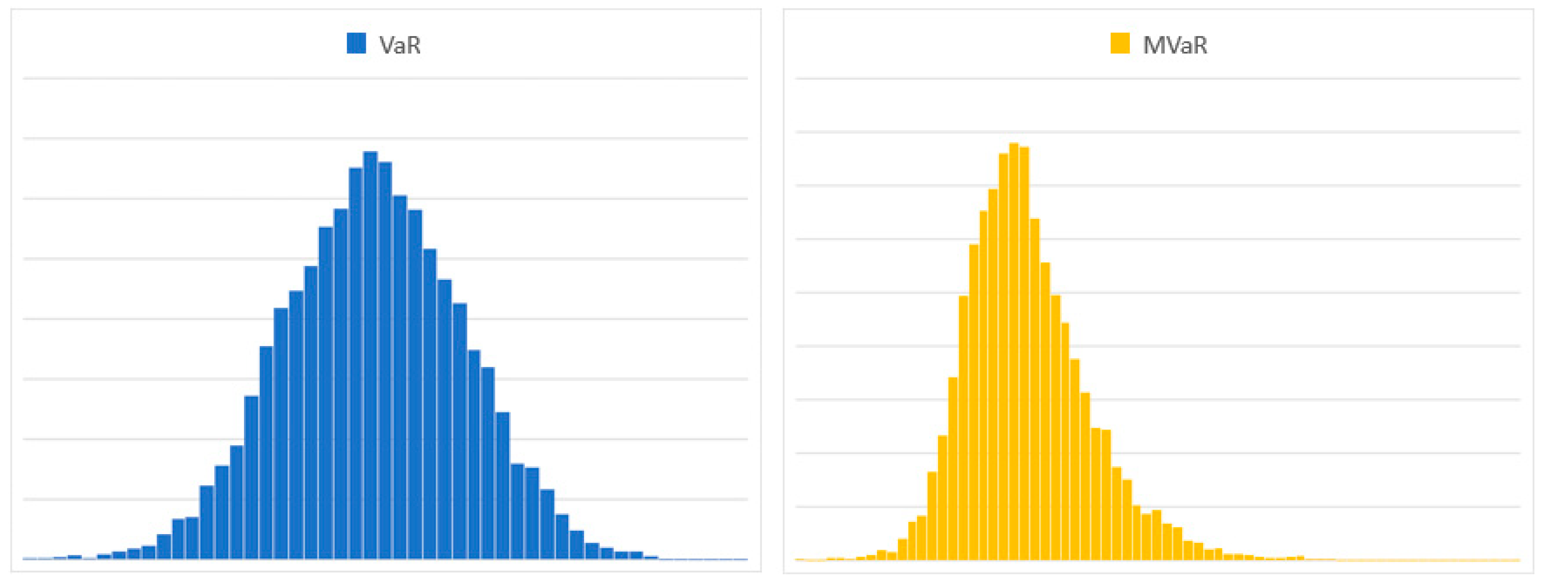
Figure 1 illustrates the graphical normality test.
In addition to examining the periodic data, it is also worth observing the histogram of the sample generated by the Monte Carlo simulation, which illustrates in
Figure 1 the difference between the two different VaR formulae. Application of the conventional VaR model yields a virtually perfectly regular bell curve, while the MVaR shows a right-skewed, thick-edged distribution. As expected, the latter considers the asymmetry and thick edges due to volatile exchange rates more strongly and is expected to provide a more realistic risk estimate for the portfolio.
By incorporating skewness and kurtosis of return distributions in modified Value at Risk MVaR, we aspire to attain a more precise estimation of potential losses within the portfolios analysed. The emphasis on extreme values captured by the measures of asymmetry makes MVaR highly suitable for assessing the risk associated with assets such as cryptocurrencies. Consequently, MVaR shows greater capability in capturing risks arising from extreme events, which prevail in financial markets to a greater extent than a normal distribution would suggest (
Favre and Galeano 2002).
Table 2 represents the data of the non-parametric test.
We chose the Jarque-Bera test for the non-parametric test to see if the log returns follow a normal distribution. In
Table 2 the results show
p < 0.05 for all instruments in the first period, and therefore, the null hypothesis is rejected, i.e., log returns do not follow a normal distribution. In the second period, we again reject the null hypothesis for Bitcoin. The log returns do not follow a normal distribution here either. In contrast, for gold and Apple stock,
p > 0.05, so we accept the null hypothesis. Log returns follow a normal distribution.
Table 3 represents the data of the log returns correlation matrix.
After the descriptive statistics and normality tests, we constructed a correlation matrix for the log yield of assets for both periods. In
Table 3 the correlation coefficients show that during the first period, there was a weak positive relationship between Bitcoin and gold and between Bitcoin and Apple stock, while there was a medium positive relationship between gold and Apple stock. In the second period, there is a stronger but still weak positive relationship between Bitcoin and gold compared with the first period. A significantly stronger, medium positive relationship is observed between Bitcoin and Apple stock compared with the first period. Finally, the weak negative relationship between gold and Apple stock is the opposite of the first period.
The results of the simulation:
In the simulation, the model seeks to find the maximum Bitcoin rate at which the risked value is the smallest. Technically, this means varying the asset ratio of a given portfolio from zero to 100% by iterating several times, during which the simulated risk values are fixed. The ratio assigned to the lowest-fixed-risked values represents the optimal Bitcoin ratio. The simulation was also performed at 95%, 99%, and 99.9% confidence intervals for all four VaR models, according to the most common risk management standards in practice, which were as follows for the first period:
The values in
Table 4 represent the highest possible Bitcoin weights, where the simulated losses are the smallest from
Table 5; consequently, these are regarded as the optimal Bitcoin weights for mitigating risk within the given confidence intervals and VaR formulas.
The values in
Table 5 represent the highest possible Bitcoin weights where the portfolio’s risk, expressed as both a percentage and an absolute value, is minimised; consequently, these are regarded as the optimal Bitcoin weights for mitigating risk within the given confidence intervals and VaR formulas.
In the first period, the Bitcoingold portfolio was tested with a maximum Bitcoin ratio of 0% for all formulas and confidence intervals, at which the portfolio loss was the smallest. This outcome means that any minimum Bitcoin ratio would only increase the value at risk during this period. A similar result was also observed for the Bitcoin–Apple portfolio. However, the averaged CVaR indicator marked the smallest value at risk at a Bitcoin rate of 3% with a 99% confidence interval. Although this minimal deviation could be considered a measurement error, it is still worth considering.
The values in
Table 6 represent the highest possible Bitcoin weights, where the simulated losses are the smallest from
Table 7; consequently, these are regarded as the optimal Bitcoin weights for mitigating risk within the given confidence intervals and VaR formulas.
The values in
Table 7 represent the highest possible Bitcoin weights where the portfolio’s risk, expressed as both a percentage and an absolute value, is minimised; consequently, these are regarded as the optimal Bitcoin weights for mitigating risk within the given confidence intervals and VaR formulas.
The second period’s simulation—essentially the stress test itself—produced very different figures. For the Bitcoin–gold portfolio, the confidence interval averages were 22%, 16%, and 12%. So, in this case, the diversification effect of Bitcoin is already clearly visible. Even if the MVaR indicator, which is the least permissive regarding volatility, is taken as a benchmark, a Bitcoin weight of at least 4–10% is still the minimum risk weight to achieve a lower risked value. The Bitcoin–Apple portfolio has an even higher Bitcoin ratio, with confidence interval averages of 74%, 47%, and 28%. Here, the results show that even at the lowest value, the portfolio should contain almost one-third Bitcoin to minimise risk.
Relationship between Bitcoin rate and value at risk:
In addition to the optimal Bitcoin ratio defined by the model, we examined the correlation between the asset ratio and the individual risked values to evaluate the differences between the values of the VaR indicators (
Table 8). The correlation was still based on the output of the Monte Carlo simulation, which consisted of 10,100 elements for each VaR indicator.
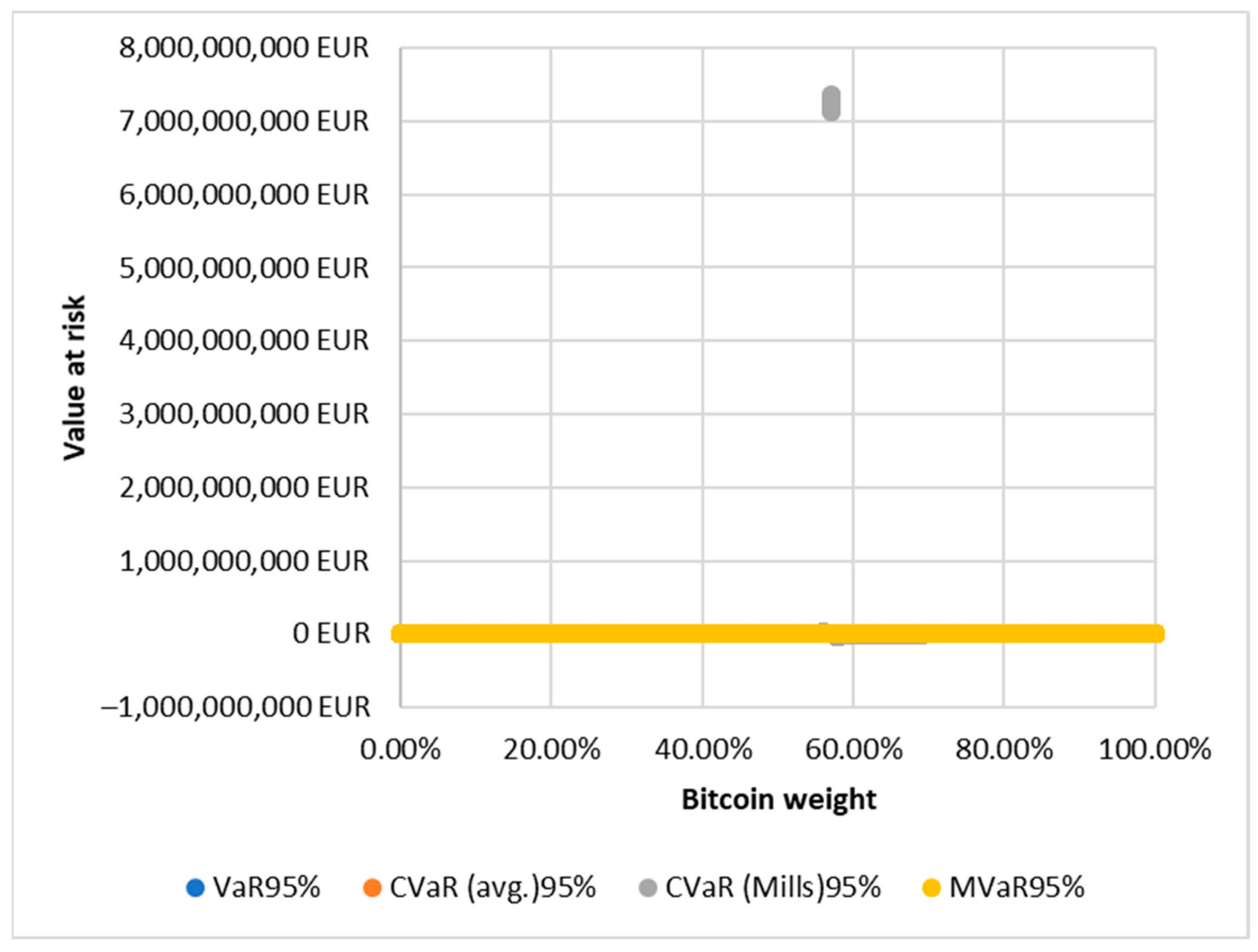
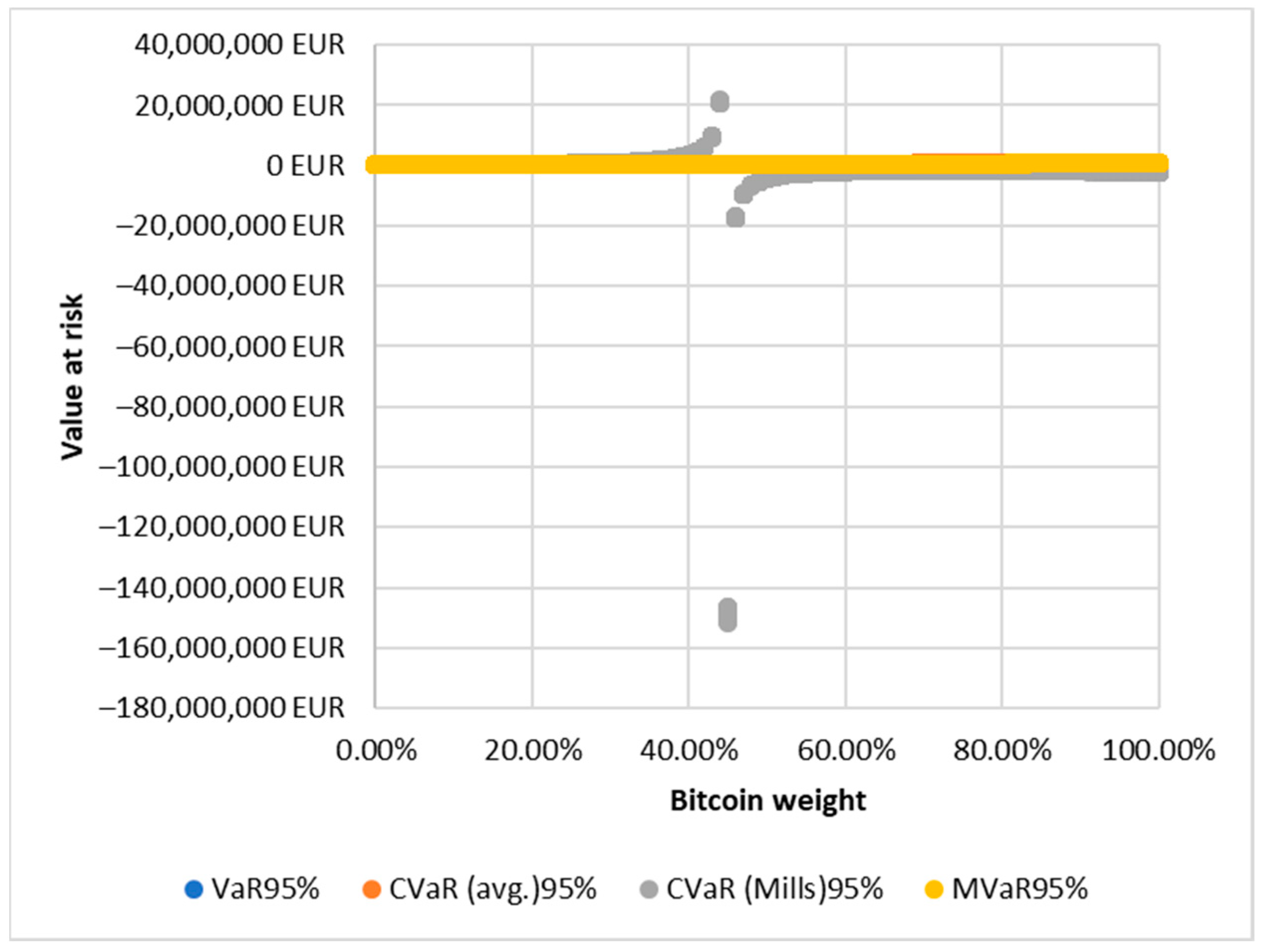
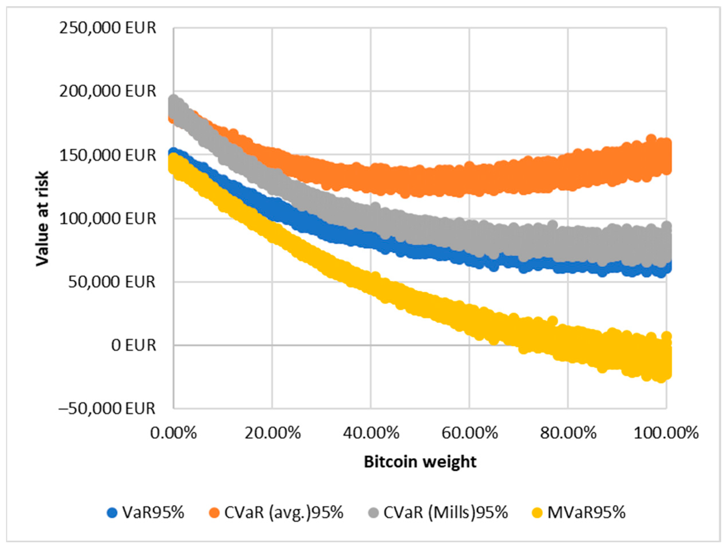
In
Table 8 in the first period, at 95% confidence intervals, the MVaR indicator has the highest correlation coefficient for both portfolios (0.9995 and 0.9966), while the CVaR (Mills) has the lowest (0.0220 and −0.0577). In the latter case, it is important to highlight that both portfolios have hyperbolic functions plotted on the graph. The discontinuity of the function has led to an extreme distortion in the correlation coefficient, which may be the reason for the extremely weak relationship. Since the function cannot be continuous, the values obtained are difficult to interpret. Therefore, the averaged CVaR value is considered more relevant as the lowest value in this case. As the function exhibits discontinuity, resulting in exceptionally high values for CVaR (Mills), the VaR and CVaR (avg.) values in
Figure 2 and
Figure 3 are so low in comparison that they are not clearly visible with this scaling.
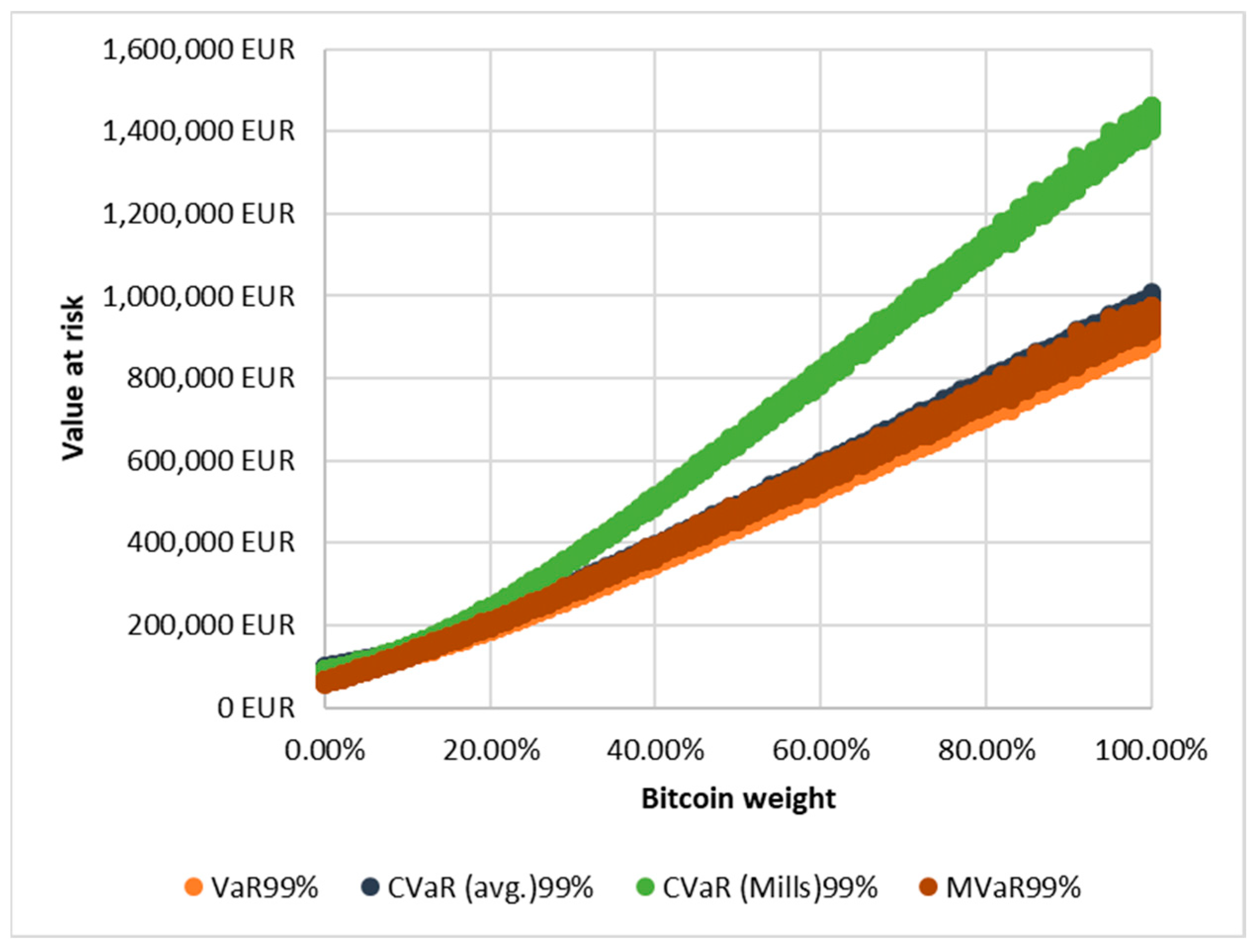
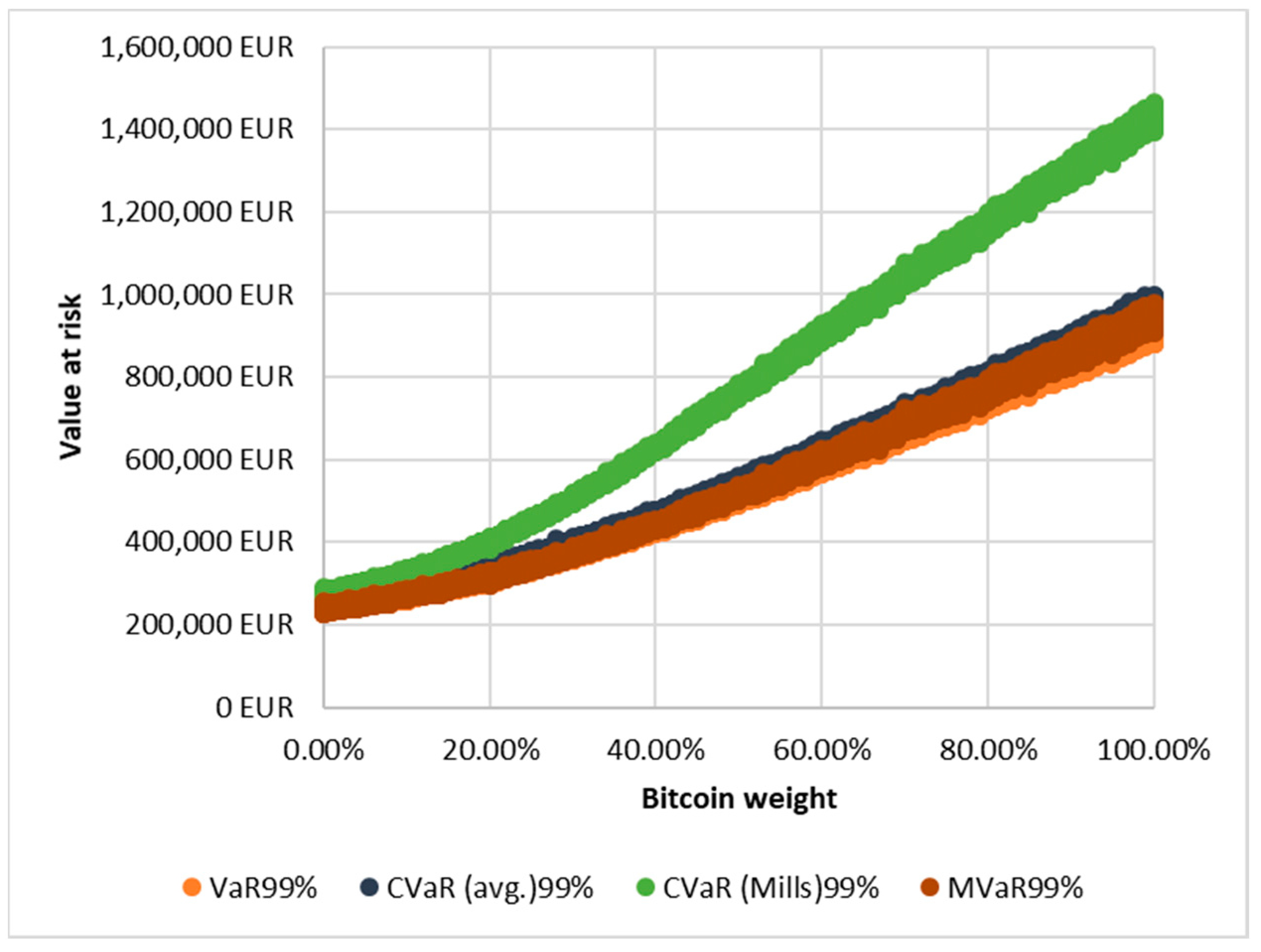
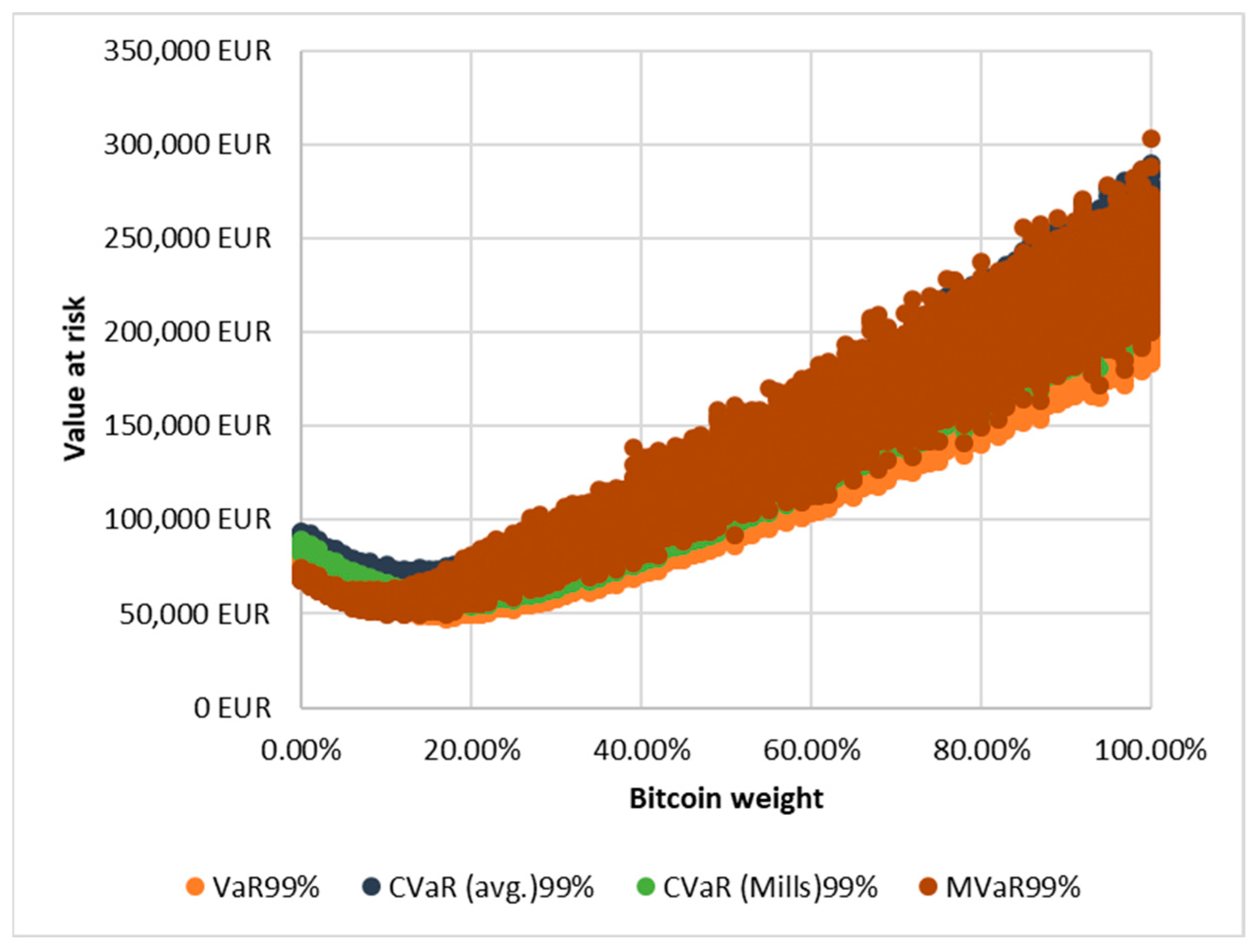
In
Figure 4 and
Figure 5 at the 99% confidence interval, a similar situation is observed for the Bitcoin–gold portfolio, where MVaR shows the highest value (0.9988) and CVaR (Mills) the lowest (0.9963). For the Bitcoin–Apple pair, however, the opposite is true, with CVaR (Mills) being the highest (0.9959) and MVaR the lowest (0.9930). The difference between the values is relatively small, but it is worth noting that the higher confidence intervals mean that the graphs of the functions show a significant divergence.
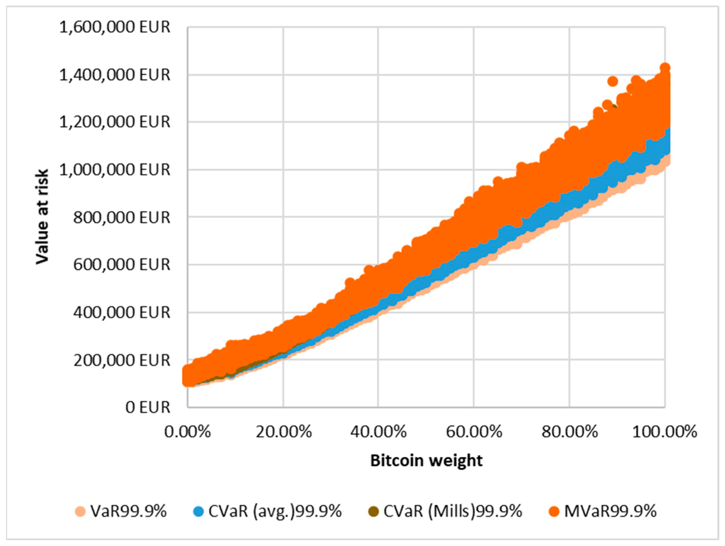
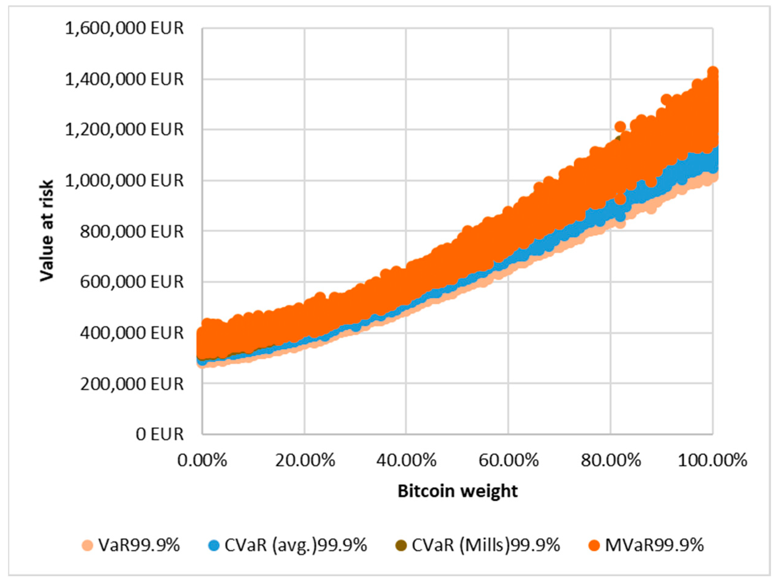
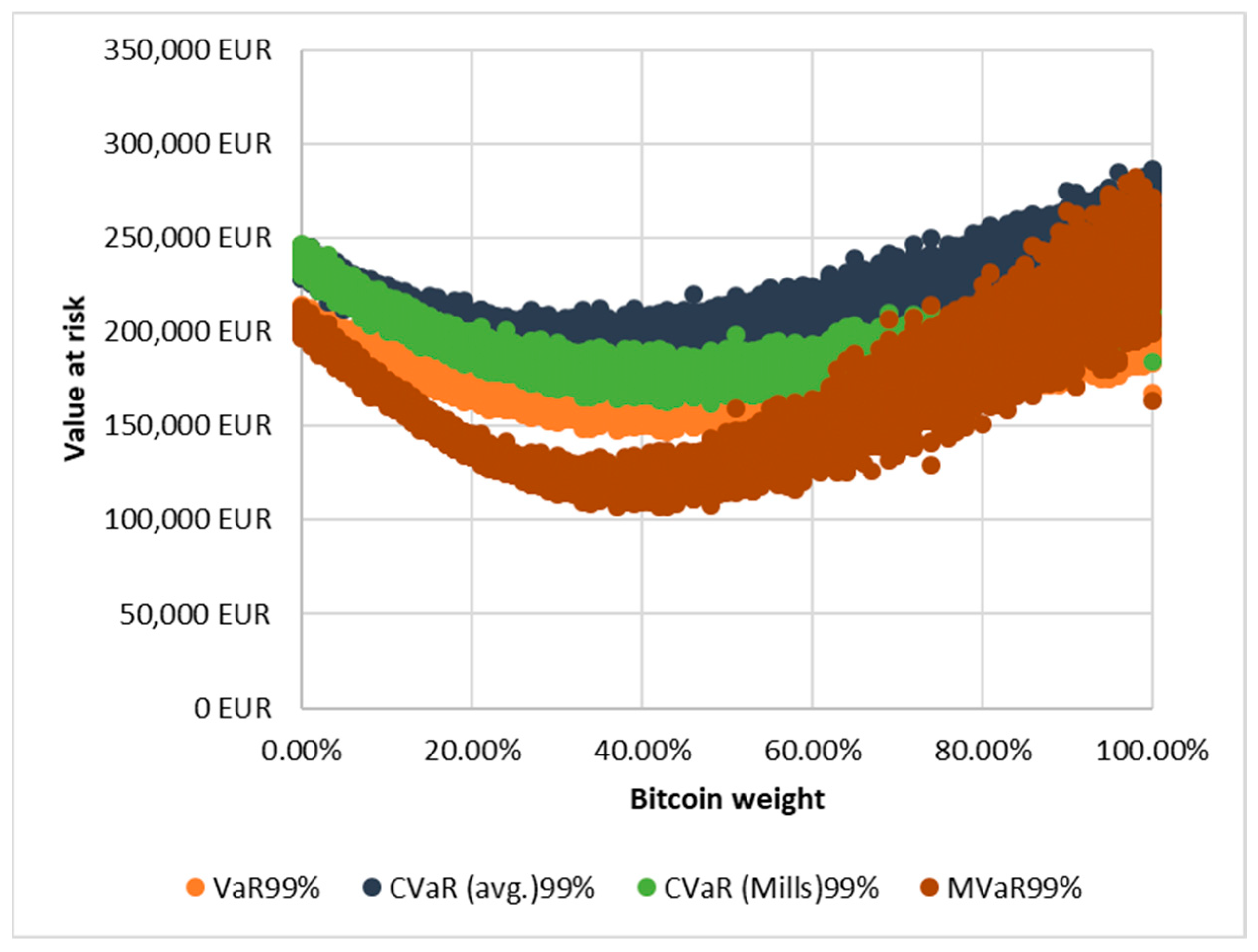
In
Figure 6 and
Figure 7 with a 99.9% confidence interval, the Bitcoin–gold portfolio had the highest correlation coefficient for VaR (0.9970) and the lowest for MVaR (0.9947). For Bitcoin–Apple, CVaR was the highest (0.9931), and MVaR was the lowest (0.9835). With such a high probability level, the extreme values are also much more extreme—a relationship visible in the graph.
Table 9 represents the data of the asset ratio and value at risk correlation matrix.
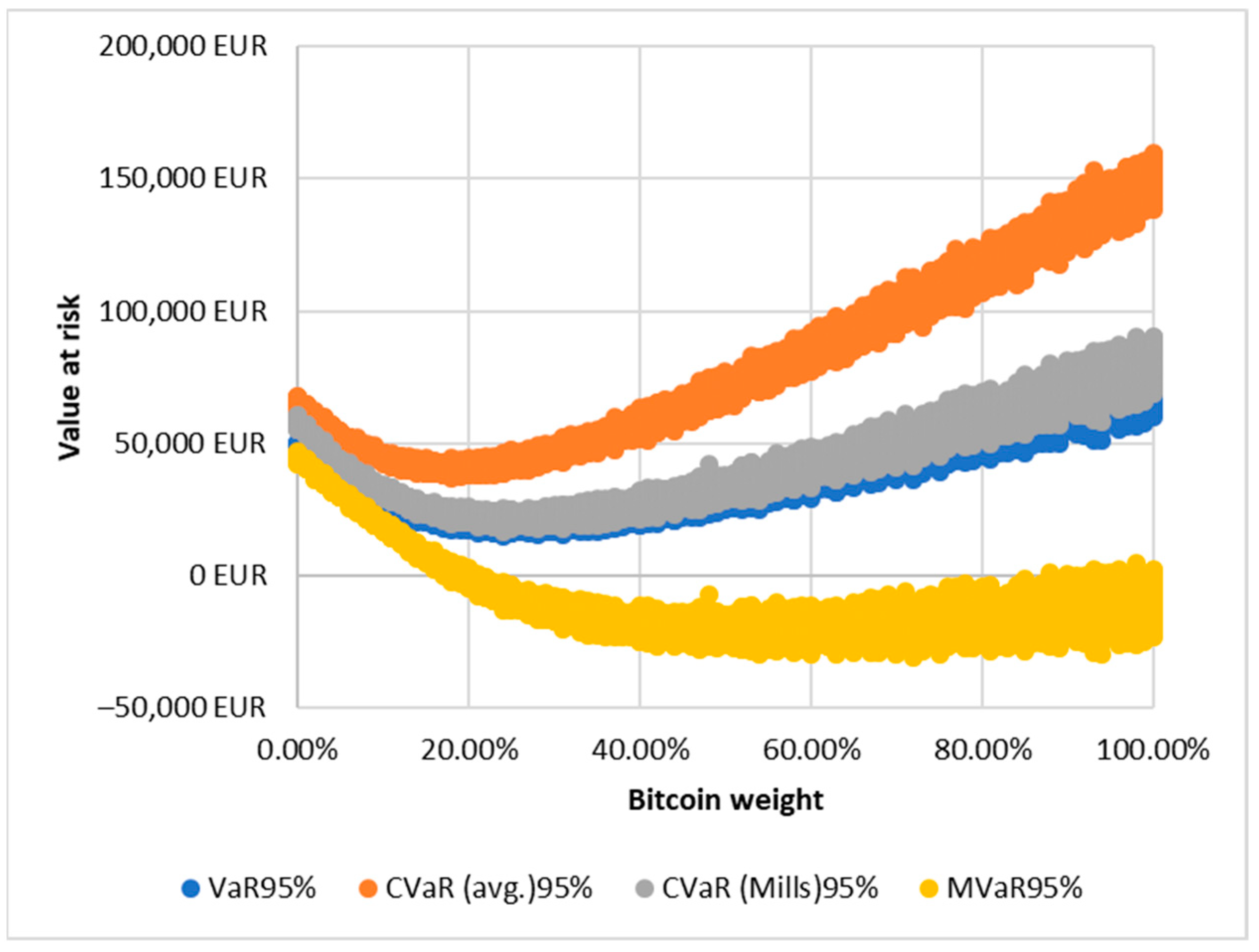
In
Table 9 in contrast to the first period, the second period shows greater dispersion. At 95% confidence intervals, the averaged CVaR indicator for both portfolios was the highest (0.9381), while MVaR was the lowest (−0.6647). The medium-to-strong negative correlation, which occurred in several cases, was not caused by a break in the function this time but by nonlinearity, whereby an increasing Bitcoin rate, as opposed to the previous one, no longer increases but decreases the value at risk (at least up to a certain level).
Below are the values at risk for the Bitcoin-Gold (
Figure 8) and Bitcoin-Apple (
Figure 9) stock portfolios at 95% confidence intervals in period 2.
In
Figure 10 and
Figure 11 at the 99% confidence interval, the Bitcoin–gold portfolio had the highest MVaR (0.9682) and the lowest CVaR (Mills) (0.9539). The Bitcoin–Apple portfolio had the highest average CVaR (0.6175) and the lowest CVaR (Mills) (−0.0478).
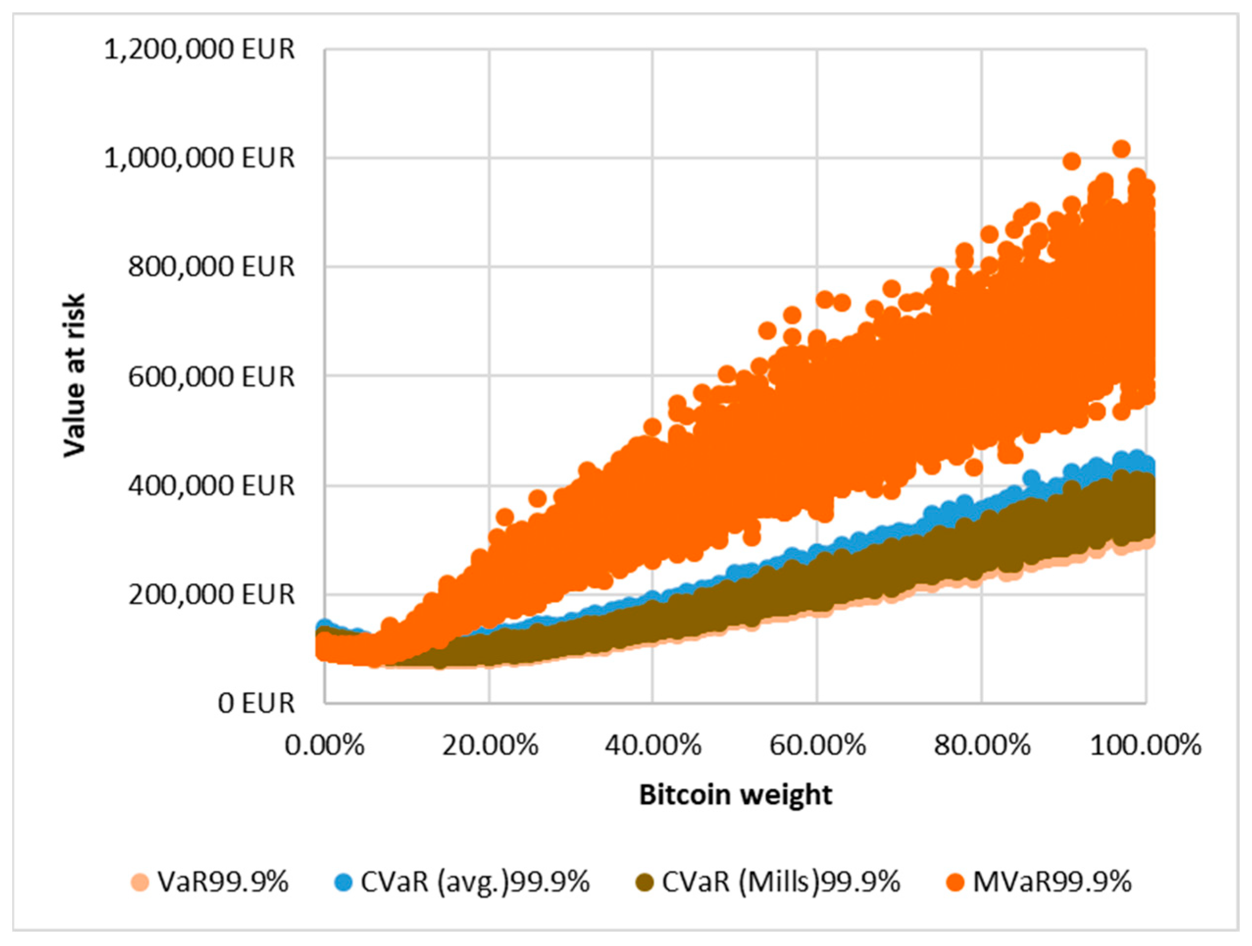
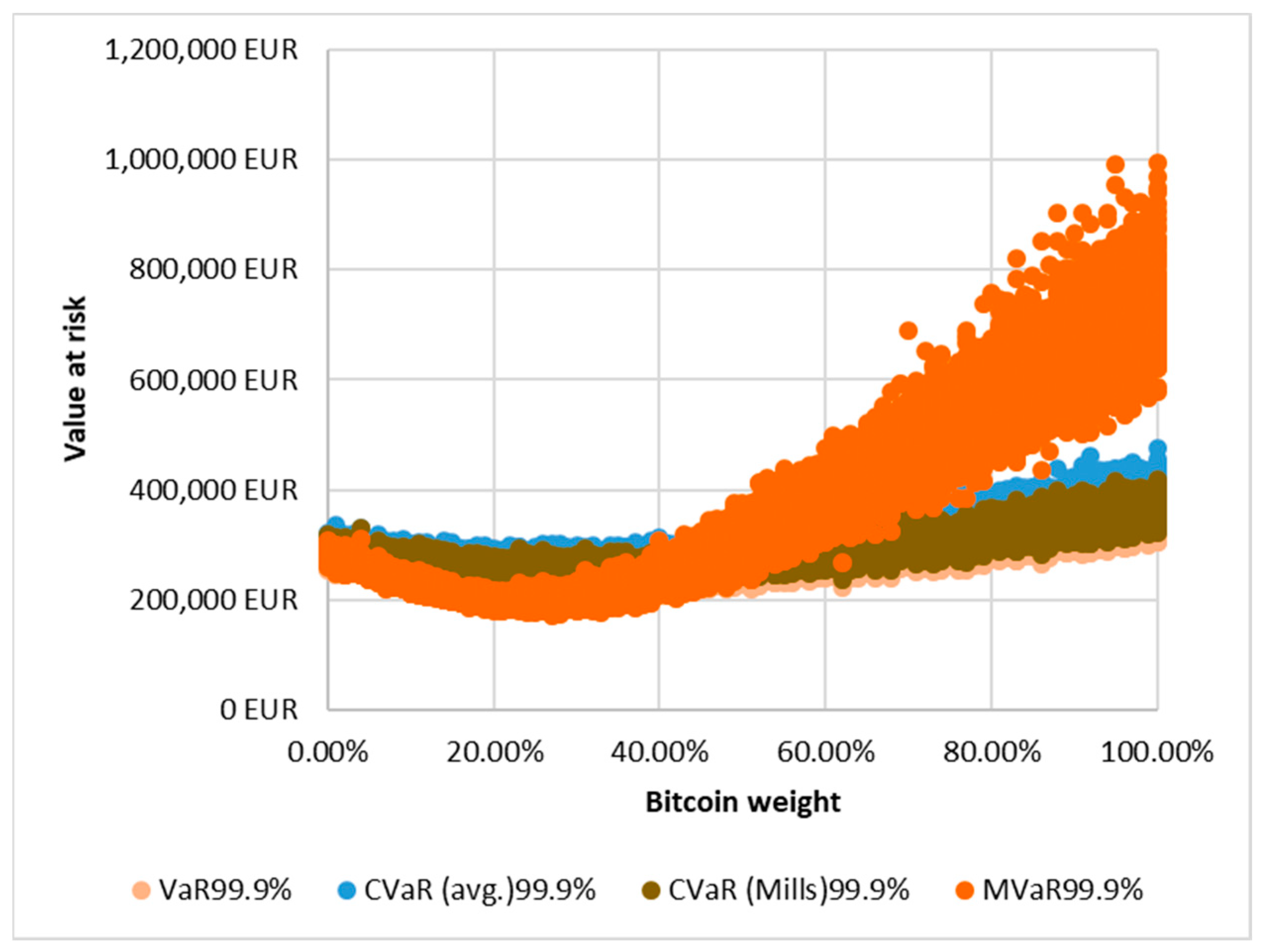
In
Figure 12 and
Figure 13 at a 99.9% confidence interval, the Bitcoin–gold portfolio had the highest correlation coefficient for the averaged CVaR (0.9710) and the lowest for the MVaR (0.9671). For Bitcoin–Apple, MVaR was the highest (0.8933), and CVaR (Mills) was the lowest (0.7435). Perhaps best illustrated in the graphs shown here is how much more sensitive MVaR is to extreme price movements than any other indicator. After the inflection point, the simulated risk values show increasing dispersion compared with the values of the other indicators, which remain roughly in the same range throughout the simulation.
3. Discussion
From an economic perspective, the triggers of financial crises and high market volatility after the onset of crises can be endogenous and exogenous (
Song et al. 2022). The origin of endogenous crises is to be found within the economy. Exogenous shocks come from outside the economy, causing crises in financial markets and the real economy. In
Song et al.’s (
2022) view, it is possible to analyse endogenous shocks on the basis of price paths and predict the occurrence of collapse due to endogenous shocks. However, crashes caused by exogenous shocks cannot be predicted. However, they also found that stock market indices in several countries showed signs of endogenous crashes despite the 2020 COVID crisis. Thus, the growth of the indices revealed features predictive of endogenous collapse. For several indices, however, the COVID crisis was found to have been a genuine exogenous shock (
Song et al. 2022).
According to
Sornette et al. (
2004), the price movements of individual financial products follow a continuous flow of news. Shocks reflected in exchange rate movements can, in turn, be both endogenous and exogenous to the economy. Although no clear evidence can be found, sudden, large market price falls are generally attributed to exogenous factors by those who are grounded in standard economics (
Sornette et al. 2004).
Models describing the dynamics of exchange rate movements of stock market products distinguish between endogenous and exogenous risks that determine price movements (
Arias-Calluari et al. 2021). Endogenous shocks can be derived from the behaviour of economic agents and their interactions. Exogenous risks are risks with a global impact. These risks are the macro-level determinants of market movements at the macro level. Exogenous risks cannot be endogenised by markets in advance and, therefore, cause rapid changes in the overall market.
In our view, the COVID-19 crisis and the Russian-Ukrainian war in 2022 could be considered exogenous shocks in terms of their economic impact. Although their mechanisms of impact on markets were different, both triggered a crisis. In both cases, there was an increase in volatility in both financial product markets and commodity markets after the crisis. Our approach is that appropriate portfolio diversification can be an effective hedge against high market volatility. In addition to the composition of the portfolio, it is important to design the portfolio with the right mix of assets.
Fang et al. (
2020) studied the long-term volatility of cryptocurrencies. They found that cryptocurrencies can provide an effective hedge against price movements of traditional instruments, and Bitcoin investment can provide a hedge against changes in the S&P index.
Bouri et al. (
2020) analysed the relationship between eight cryptocurrencies and US equities. They evaluated the relationship between the S&P 500 stock index, ten stock sectors, and cryptocurrencies. They concluded that Bitcoin can be considered a promising hedging instrument against any US equity sector.
Kumah and Mensah (
2020) investigated the relationship between gold and cryptocurrency price movements. They examined the relationships in both rising and falling markets. In all cases, they found that cryptocurrencies can be a hedge for gold investors.
Hsu et al. (
2021) investigated the correlations between major cryptocurrencies, traditional currencies, and gold prices. They found differences in values before and during the pandemic. Cryptocurrencies and gold yields showed a stronger positive relationship during the pandemic. Their results suggest that cryptocurrencies, like gold, may provide a buffer against changes in the returns of other assets. In concordance with the findings presented by
Hsu et al. (
2021), our study similarly deduces that crypto assets serve as an efficacious mechanism for portfolio diversification.
González et al. (
2021) analysed the relationship between the twelve largest cryptocurrencies and the gold exchange rate between 1 January 2015 and 30 June 2020. They found that, due to the COVID-19 crisis, the correlation between the majority of cryptocurrencies and the gold price increased. During the turbulence, the persistence between gold and crypto asset prices increased. According to their findings, some of the cryptoassets (Cardano, Tether, and Tezos) offer diversification benefits to investors. Their findings are consistent with our own research, which identified similar diversification benefits when examining the pairing of Bitcoin and gold. We compared the results of our studies with the research of
Lee et al. (
2020), in their study they concluded that it is possible to create a diversified portfolio even with a limited set of assets. Their results provide further evidence of the importance of Bitcoin as a potential diversification tool to reduce risk in portfolios (
Lee et al. 2020). The
Liu et al. (
2021) study supports the view that crypto assets can improve the risk-return characteristics of traditional portfolios, even during periods of sharp market fluctuations such as the market volatility caused by COVID-19. Similar to the results of our study, they concluded that crypto assets have potential value in portfolio diversification and improving risk-return, although further research is needed to develop future strategies for investing in digital currencies.
Bhuiyan et al. (
2021) highlight the diversification properties of Bitcoin in their study, which leads them to the conclusion that Bitcoin is relatively isolated from most financial instruments, so it can provide diversification benefits for investors (
Bhuiyan et al. 2021). We also examined Bitcoin’s ability to diversify in our study, and based on our results, we came to the same conclusion that Bitcoin supports diversification.
The results of our calculations are similar to those found in the literature. Bitcoin, representing cryptocurrencies, provides an efficient hedge for equity investors. The shelter role is stronger in turbulent market conditions. In contrast to the literature, our study could not only demonstrate the role of cryptocurrencies in diversification. We also showed the optimal ratio of Bitcoin in a gold and equity portfolio.
4. Materials and Methods
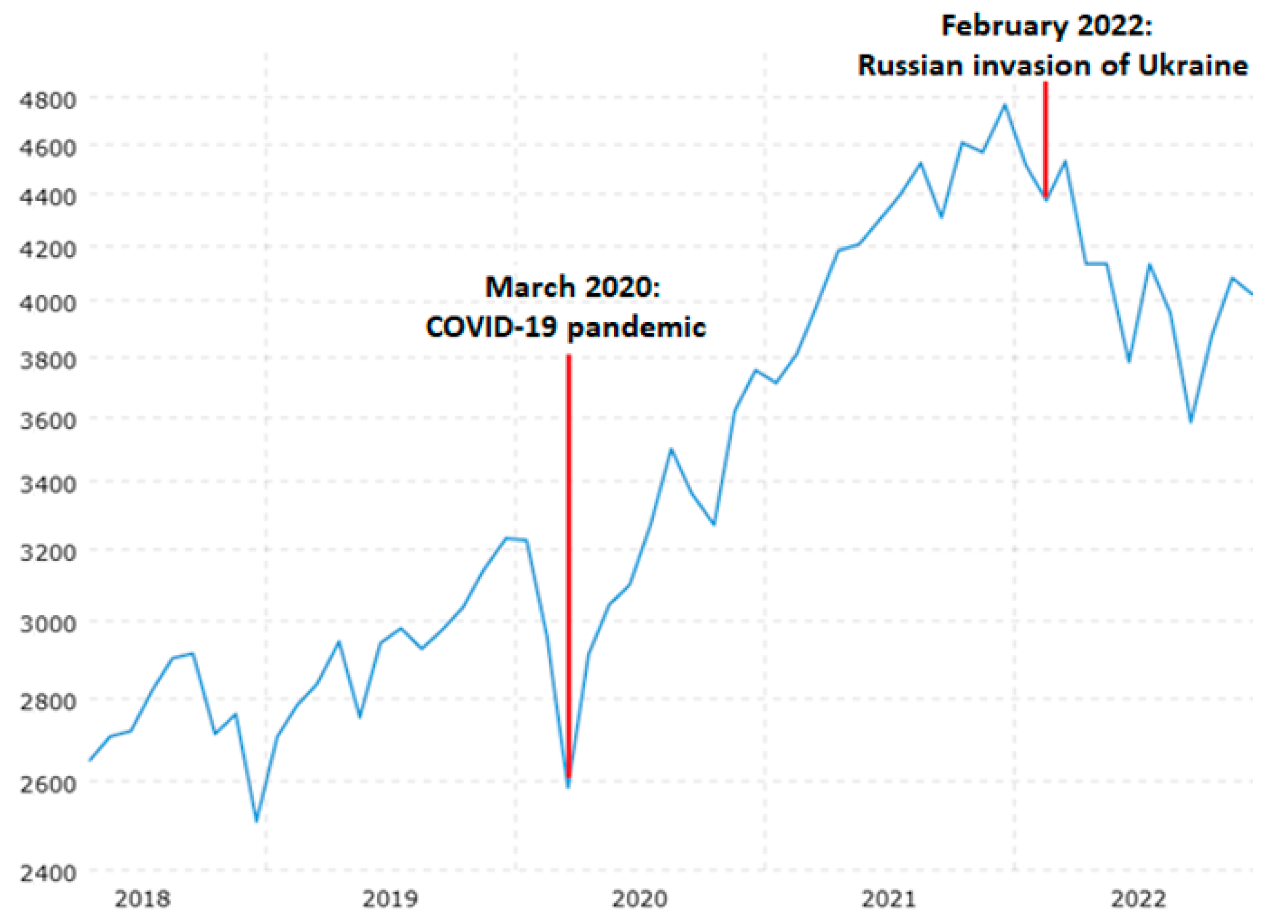
The study database includes exchange rate data for two consecutive years. When selecting the periods under examination, it was important to compare favourable and less favourable periods from a macroeconomic point of view so that the study results can be interpreted as a stress test in addition to observing the diversification effect. The first period under examination is from 1 September 2020 to 31 August 2021, and the second from 1 September 2021 to 31 August 2022. As shown in
Figure 14, in the first half of the first period, the prolonged economic and social shock caused by the coronavirus epidemic was still very much present. However, the announcement of the first vaccine led to a positive market reaction and a slow recovery.
The second period includes the Russian-Ukrainian war that began on 24 February 2022 and the subsequent shock. Most businesses have not yet fully recovered from the downturn caused by the coronavirus outbreak. However, the outbreak of war, combined with the long-standing energy crisis and chip shortages, has ushered in a period of greater uncertainty than ever before. In most economies, inflation and (consequently) base rates have risen sharply. In general, the unfolding macroeconomic trends have also harmed the money and capital markets, which are key for analysis.
For the analysis, we have chosen three investment instruments, one of which is Bitcoin—a cryptocurrency. Since Bitcoin is one of the most dominant crypto assets with the largest market capitalisation, it is suitable to represent the underlying trend of the crypto market in the analysis. Gold was chosen as the second instrument because its price is countercyclical, unlike many other assets. It is important to emphasise that this is not an exchange-traded fund or other gold-related security, but physical gold. The exchange rate is per ounce (28.3495 g) in US dollar terms. We chose a generally well-performing popular technology stock, Apple, for the third instrument. Two portfolios were created from the three assets selected. One consists of Bitcoin and gold, and the other consists of Bitcoin and Apple stock.
The VaR method was chosen for the risk analysis used in the model. By definition, it expresses the maximum expected loss at a given significance level over a given time horizon (worst-case scenario). The so-called conservative formula originally developed is structured as follows: (
J.P.Morgan/Reuters 2018)
α = confidence interval
μ = average
Z = standard score
σ = standard deviation
During the 2008 global economic crisis, it was shown that the VaR ratios used until then significantly underestimated market risks. The main reason is that the conservative VaR formula is based on a specific confidence interval and does not consider potential losses beyond that interval. As a tail risk indicator, the Conditional Value at Risk indicator (CVaR) is:
An approximation for the integral function is obtained by calculating the arithmetic mean of the range (worst realised returns) above a given confidence interval. The resulting value is no longer just the maximum expected loss at a given point. Rather, it is the average of the losses beyond the maximum loss, giving a much more accurate picture of the potential risk (
Banihashemi and Navidi 2017).
In addition to the expected shortfall formula, another formula for calculating the conditional value at risk can be derived from an inverse Mills ratio. Unlike averaging, it gives an accurate result for a given VaR value:
Regarding the VaR and CVaR indicators described thus far, it is important to note that they can be used reliably, assuming a normal distribution of returns. However, when considering volatile instruments, such as cryptocurrencies, it is important to bear in mind that the distribution can be somewhat asymmetric, so in addition to the mean and standard deviation of returns, we also need to take into account their skewness and peakiness. To overcome this problem, in 2002, Laurent Favre and José-Antonio Galeano developed the MVaR (mean-variance-adjusted risk-adjusted return) formula, which builds on the conservative VaR formula and takes into account both the peak and skewness. The authors mentioned that the formula may be inaccurate at lower confidence levels (
Favre and Galeano 2002).
All the VaR variations described so far have been considered in the analysis for comprehensive results. In addition to choosing formulas, another essential condition for calculating the VaR is using the right methodology. In the literature, three different methods are distinguished:
Monte Carlo method
Parametric method
The Monte Carlo method is a stochastic simulation method in which a pseudo-random number generator produces the values of the probability variables. It is considered a computationally intensive method, but with developments in computer science, it is becoming less and less technically problematic.
The parametric (or variance-covariance) method is one of the simplest and most widely used simulation methods. It is based on the variance-covariance matrix of the assets in the portfolio. In practice, it is best expressed as the volatility according to the conservative VaR formula multiplied by the market value. Since it assumes a normal distribution, measuring the risk from thick edges is unsuitable.
The non-parametric (or historical) method is more flexible than the parametric method because it does not assume a specific distribution and can be applied to a wider range of instruments. In principle, it is suitable for measuring risk from thick-edged instruments, but this is only possible if the historical data used also show a thick-edged distribution (
Romero et al. 2013).
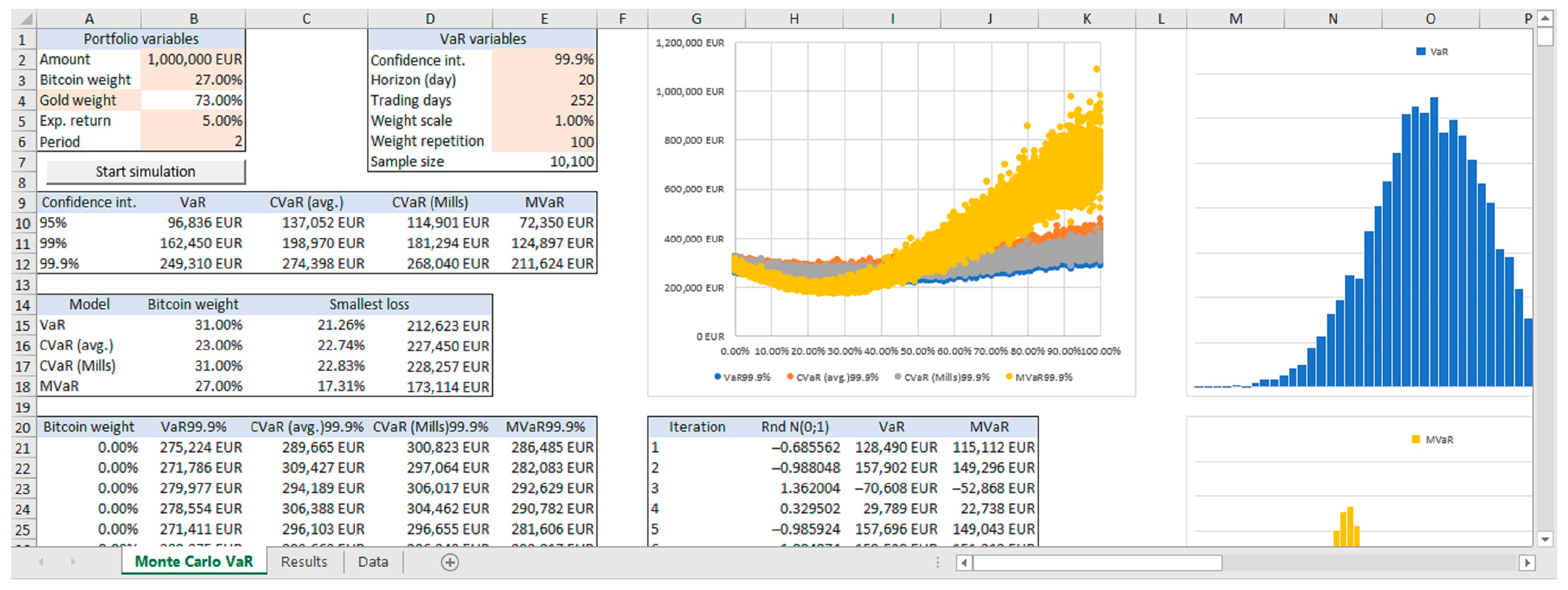
The Monte Carlo method was chosen for the model used in the analysis. It is generally well suited for value-at-risk modelling and measuring the risks arising from thick edges. The model was created in Microsoft Excel (
Figure 15). As a first step, the log returns of the downloaded exchange rates were calculated. The model is automated using Visual Basic and can be easily parameterised.
The first step in the parameters is to specify the portfolio amount, the composition (Bitcoin–gold or Bitcoin–Apple stock), the expected return, and the period to be tested. For the analysis, we have specified 1,000,000 EUR with an expected return of 5%. The programme itself runs the asset allocation from zero to 100%. The programme can repeat the calculation of the risked value for each pair of asset ratios any number of times, which in this case was 100, so the sample consisted of 10,100 elements (101 × 100) for all four VaR models, or a total of n = 40,400. In contrast to the simple target value search, each variation’s risked value is recorded, allowing a graphical interpretation of the trend in the simulation. As additional VaR parameters, a time horizon of 20 days and 252 trading days per year were considered.
The risk values generated by the simulation are calculated as follows for the conservative formula:
5. Conclusions
Based on the results of the descriptive statistics, we can say that the general statement that cryptocurrencies—in our case, Bitcoin—are rather volatile assets has been proven. In the stress test, the mean of its log odds went from positive to negative, and an increased left-asymmetric distribution based on skewness and peakedness was observed. In contrast, the mean and standard deviation of the log returns of gold and Apple stock did not change significantly during the stress test, but the degree of left asymmetry decreased.
The graphical normality test demonstrated the inaccuracy of risk analysis based on conservative Value at Risk indicators. As in the period preceding the 2008 global economic crisis, the simulation produced a near-normal distribution, with the main problem being that it ignores extreme losses due to thick edges. In contrast, the simulation for the MVaR indicator produced a highly asymmetric distribution in all cases, highlighting the expected risks. Based on the results of the non-parametric test, only two out of six cases of normal distribution were observed, neither of which was Bitcoin. These results allow us to confirm again the conclusion drawn from the descriptive statistics and the graphical normality test that extremely large fluctuations characterise the Bitcoin exchange rate. Considering the correlation matrix’s results, Bitcoin showed a stronger co-movement with gold and Apple stock during the stress test. However, there was an opposite correlation between gold and Apple stock. The result of the correlation matrix illustrates the extent to which the correlation between the log returns of different assets can change in response to a stress event. It also predicts that, partly because of this, the Monte Carlo simulation is expected to find significantly different asset ratios over the two periods.
The research results ultimately confirm that including cryptoassets can reduce the risk of an investment portfolio. The two periods examined in the simulation produced starkly different results, suggesting that Bitcoin’s ability to diversify has become significantly important in the market situation that has unfolded due to the Russian-Ukrainian war.
6. Limitations and Further Research
Our study, which focuses on the risk-reducing ability of crypto asset investment portfolios, has several limitations. Our research, which focused on the effect of integrating crypto assets into portfolios, provided valuable insight into their risk-reducing potential; however, the narrower focus of the study, especially due to the examination of gold and Apple shares, allows for more limited generalisation. The main reason for choosing gold and Apple was due to their market importance and frequent use. Gold is one of the most popular investment instruments, and Apple is one of the most important stocks with its role and market capitalisation in the S&P 500 index. As a result, gold and Apple are the most frequently used instruments in portfolio diversification and risk management studies. At the same time, to confirm the results of our study, a wider range of instruments should be taken into account. Investigating a wider range of crypto-assets and other traditional investment instruments, such as additional stocks and bonds, could increase the generalizability of our results. Furthermore, the long-term effects of integrating crypto assets into investment portfolios could be better understood by including additional market cycles and economic conditions.
As a future research opportunity, the performance and risk characteristics of crypto assets should be investigated by examining a wider range of instruments as well as by expanding market cycles. The introduction of crypto ETFs and the investigation of their impact on financial markets can be formulated as further research opportunities, especially in the investigation of the risk reduction ability of the investment portfolios of crypto assets examined in this study. When examining crypto ETFs and other traditional instruments, particular attention can be paid to asset allocation strategies, risk management, and portfolio diversification. Analysing the market integration of crypto ETFs can be particularly important in understanding the role these instruments can play in improving the stability and performance of investment portfolios in volatile market conditions, as well as their impact on correlation with traditional financial instruments and market liquidity.


