Abstract
This research delves into the fusion of spatial clustering and predictive modeling within auto insurance data analytics. The primary focus of this research is on addressing challenges stemming from the dynamic nature of spatial patterns in multiple accident year claim data, by using spatially constrained clustering. The spatially constrained clustering is implemented under hierarchical clustering with a soft contiguity constraint. It is highly desirable for insurance companies and insurance regulators to be able to make meaningful comparisons of loss patterns obtained from multiple reporting years that summarize multiple accident year loss metrics. By integrating spatial clustering techniques, the study not only improves the credibility of predictive models but also introduces a strategic dimension reduction method that concurrently enhances the interpretability of predictive models used. The evolving nature of spatial patterns over time poses a significant barrier to a better understanding of complex insurance systems as these patterns transform due to various factors. While spatial clustering effectively identifies regions with similar loss data characteristics, maintaining up-to-date clusters is an ongoing challenge. This research underscores the importance of studying spatial patterns of auto insurance claim data across major insurance coverage types, including Accident Benefits (AB), Collision (CL), and Third-Party Liability (TPL). The research offers regulators valuable insights into distinct risk profiles associated with different coverage categories and territories. By leveraging spatial loss data from pre-pandemic and pandemic periods, this study also aims to uncover the impact of the COVID-19 pandemic on auto insurance claims of major coverage types. From this perspective, we observe a statistically significant increase in insurance premiums for CL coverage after the pandemic. The proposed unified spatial clustering method incorporates a relabeling strategy to standardize comparisons across different accident years, contributing to a more robust understanding of the pandemic effects on auto insurance claims. This innovative approach has the potential to significantly influence data visualization and pattern recognition, thereby improving the reliability and interpretability of clustering methods.
1. Introduction
Spatial modeling, incorporating both data clustering techniques and predictive models (Hussain et al. 2022; La Bella et al. 2022; Seresht et al. 2020), is highly appealing from a statistical point of view when it is applied as an advanced loss data analytic. Utilizing clustering allows for a significant reduction in the number of basic rating units, thereby enhancing the reliability of models and credibility of the loss estimate employed in auto insurance pricing and the rate regulation process. Concurrently, predictive modeling facilitates statistical estimates of the impact of underlying risk factors (Aslam et al. 2022; Chowdhury et al. 2022; Cummins et al. 2001), which may include the territory and a special event that may occur. The strategic approach to dimension reduction through clustering not only makes predictive modeling practical but also enhances interpretability by reducing the number of levels attributed to territory as a risk factor. Moreover, it proves instrumental in studying the impact of global health crises, such as the COVID-19 pandemic, on auto insurance loss patterns. Nevertheless, challenges emerge in auto insurance when clustering multiple accident years of loss data for rate regulation and pricing purposes, necessitating consideration of specialized machine learning methodologies. A significant hurdle arises from the dynamic nature of spatial patterns (Inostroza et al. 2013; Ramachandra et al. 2013). While spatial clustering identifies geographic regions with similar data characteristics, these patterns may evolve over time due to factors like urban development, shifts in traffic patterns, or changes in population density Zhang et al. (2013). Sustaining accurate and up-to-date spatial clusters for auto insurance rate regulation becomes an ongoing challenge. Despite the advantages of spatial clustering in grouping regions with similar loss experiences, each group may still exhibit heterogeneity (Wang and Wu 2020; Zhu et al. 2020), primarily due to the time effect. Analyzing the variability of loss data within a cluster demands further examination to fully comprehend the intricacies, achievable through a comprehensive analysis of spatial-temporal patterns of losses Li and Su (2022). Identifying differences in loss metrics across both spatial and temporal domains is crucial. However, effectively analyzing these spatial-temporal dynamics requires sophisticated modeling techniques to capture the time and spatially dependent aspects of loss data. Consequently, the development of interpretable and specialized clustering methods becomes crucial for regulatory compliance and stakeholder understanding.
Besides the consideration of spatial-temporal dynamics, evaluating loss patterns across various auto insurance coverages is a crucial element in the effective oversight of insurance rates within the industry. Investigating loss patterns across various major insurance coverage types is of importance for both insurance companies and regulators. Such analyses offer crucial insights that directly impact several aspects of the auto insurance system. They facilitate a comprehensive assessment of risk, enabling insurers to accurately evaluate the likelihood of losses under different major coverage types. This, in turn, informs the pricing of insurance policies, ensuring that premiums are set at levels that adequately cover anticipated losses while remaining competitive in the market. Moreover, understanding these loss patterns aids in the development of new insurance products or the refinement of existing ones, allowing insurers to tailor coverage limits, deductibles, and policy terms to effectively manage risk and enhance profitability. The focus on major insurance coverages may be considered a microscopic analysis of loss patterns when compared to the investigation of the overall aggregation of loss. Essentially, the underlying loss patterns across different insurance coverages are different due to their nature. This particular analytical aspect empowers insurance regulators and insurance companies to conduct thorough assessments of the risks associated with different coverage types, including third-party liability, collision, and medical. Each coverage type may exhibit unique loss patterns. In consideration of these factors, analyzing auto insurance losses by coverage equips regulators to respond to evolving trends in the insurance landscape, and improves the overall homogeneity of risk associated with each coverage type.
Data visualization and pattern exploration in the auto insurance area plays an important role in loss data analytics. This research focuses on Canadian regulatory datasets to uncover spatial and temporal patterns in loss metrics for major insurance coverages. Understanding the temporal and spatial evolution of auto insurance losses has been a longstanding interest, particularly for auto insurance regulators in Canada and other countries. By examining loss patterns from accident years 2015 to 2022, encompassing various loss metrics and premiums, we aim to assess the impact of COVID-19. These datasets include both pre-pandemic and post-pandemic periods, providing a comprehensive basis for our analysis. The significant changes in loss patterns, including claim frequency, claim severity, and loss costs observed before and after the COVID-19 pandemic, motivate our exploration of clustering techniques for more effective data analysis. A major challenge is comparing patterns from multiple accident year datasets. Specifically, in addressing the impacts of the COVID-19 pandemic, we need to compare loss patterns from pre-pandemic and post-pandemic periods. For instance, loss data from southern Ontario, Canada’s most economically developed region, exhibit high volatility both spatially and temporally. Furthermore, exploratory data analysis does not yield inferential results, highlighting the need to understand how loss costs and average premiums are influenced by the same explanatory variables, such as accident years and regional differences.
In this study, we propose to use a unified spatial clustering approach to discern spatial patterns while overcoming challenges posed by the inherent variability in multiple accident half-years’ data and potential inconsistencies in cluster labeling. Our investigation addresses these challenges by leveraging both pre-pandemic and pandemic period loss data. Our primary objective is to unveil the impact of the COVID-19 pandemic on auto insurance loss metrics, specifically addressing the issue of inconsistent cluster labels across multiple accident half-years. This ensures a meaningful comparison of spatial patterns across different accident years. To elaborate further, we assign labels to each cluster, ranging from 1 to 15, with, for instance, cluster 1 denoting high claim frequency. Even if the recorded claim frequency in a given Forward Sortation Area (FSA) remains consistent across different periods, the assigned cluster label is relative to other regions. Consequently, the perceived risk level of an area may be represented differently or experience significant fluctuations. In response to this challenge, our proposed method involves fixing each cluster label to a specific range of a given loss metric during the clustering process. This relabeling strategy aims to standardize the level of a given loss metric, ensuring that the comparison of results obtained from different accident years is meaningful. This innovative unified clusters approach has the potential to significantly impact the fields of data visualization and pattern recognition. By addressing the intricacies of cluster labeling and maintaining consistency across various accident years, our methodology enhances the reliability and interpretability of discovered spatial patterns, contributing to a more robust understanding of the COVID-19 pandemic’s effect on auto insurance loss patterns. This unified approach makes our proposed method advantageous over other traditional clustering approaches.
The rest of this paper is organized as follows: In Section 3, the data are introduced and the proposed methods are discussed. Next, in Section 4, a summary of the obtained results and the application to spatial loss datasets is presented and analyzed. Finally, we conclude our findings, provide further remarks and outline future work in Section 5.
2. Related Work
Spatial clustering is an unsupervised learning approach in spatial data science and machine learning, and is widely applied in many fields of application. Spatial clustering has been used to study spatial effects in criminology. One such study is Mennis and Harris (2013), in which juvenile sentencing data were used to partition neighborhoods in Philadelphia into regions corresponding to crime risk, i.e., homogeneous with respect to chosen socioeconomic variables. The regionalization algorithm also led to some interesting conclusions. For example, the study found a phenomenon of ‘spatial contagion’, where juvenile criminal activity in high-risk neighborhoods spilled over to other surrounding areas Mennis and Harris (2013). By its own admission, studying crime rates through spatial clustering does little to explain individual behavior. However, the inferences drawn are objective and spatial clustering can clearly capture widespread behavior, which also helps to formulate responsive action. The main limitation of a study that focuses solely on spatial patterns is that it may overlook crucial dynamics in the time domain. As a result, the patterns and behaviors identified through spatial clustering might fail to capture temporal variations.
The applications of spatial clustering are also clear in environmental studies, such as identifying precipitation regions in Ethiopia, as in Zhang et al. (2016). The machine learning techniques deployed in the study involve specifying metrics for intercluster and intracluster homogeneity. Then, the study became an optimization problem with respect to the specified homogeneity measure. The result was a partition of the data into eight distinct regions which corresponded to different precipitation behavior. This information was applicable to local weather forecasting and climate study (Zhang et al. (2016)). Another advantage was that the entire process is automated and relies on few prior assumptions, allowing for greater objectivity. When compared to our specific focus on both spatial-temporal dynamics, studies utilizing spatial clustering have their own merits within their particular domain of application. However, while unifying multiple observations across different times might not be the primary aim of such studies, relying solely on spatial clustering could result in methodological limitations.
Public health is another area where spatial clustering is a useful technique, such as the study of diagnosed leprosy cases in São Paulo across eight years in Ramos et al. (2017). The spatial scan statistic, introduced in Kulldorff (1994), was used to find areas with high risk of contracting leprosy. This was especially important because diagnosis and treatment of leprosy were already available, so eradicating leprosy in Brazil was a matter of healthcare and policy. Identifying high risk areas allowed for the government to take efficient action to help the most vulnerable communities. The analysis confirmed association between socioeconomic factors and leprosy risk: the neighborhoods with the highest risk of catching leprosy had ‘precarious housing, many residents per household, low income and low education’ Ramos et al. (2017). Importantly, upon finding other links, such as the large proportion of cases being for males, the research refers to other fields of study in understanding the underlying causes for the correlation. Spatial clustering techniques have been employed to analyze COVID-19 rates in the United States Andrews et al. (2021). A study utilizing these techniques revealed limited variations in the spatial distribution of COVID-19 rates, indicating that infections were uniformly widespread across the country. In Liu et al. (2021), Moran’s I statistic was used to identify spatial clusters of COVID-19. This study demonstrated that applying appropriate lockdown measures and travel restrictions was effective for the control and prevention of COVID-19.
The aforementioned study provided crucial evidence supporting the importance of using statistical and computational techniques in decision-making processes. This is particularly relevant in the context of auto insurance rate classification and regulatory filings. In auto insurance, rate regulation mandates that any proposed rate changes by insurance companies must be statistically supported, with the methodology used being both statistically and actuarially sound. This requirement motivated us to conduct this pilot study on unifying spatial clustering.
3. Materials and Methods
This research focuses on analyzing regulatory Automobile Statistical Plan (ASP) data sourced from the General Insurance Statistical Agency of Canada, which can be accessed at the following URL: https://www.gisa.ca (accessed on 3 July 2023). The data we analyzed were for both pre- and after-pandemic in order to address the potential impact caused by COVID-19 on auto insurance major coverage types. The initial data information was generated from insurance information systems that collect data about policyholders, premiums charged, and claim information, etc. After arranging the data into a suitable format and deriving loss quantities, we analyze various metrics including claim frequencies, claim severity, and loss costs across FSAs. In Canada, FSAs serve as the basic rating unit for auto insurance pricing, representing territory risk. These loss metrics are computed for each FSA within Ontario, and they are the input data for spatial clustering. Our approach is to discover a spatial pattern of each insurance loss metric using multiple accident year data. The research considers the following major auto insurance coverages: Accident Benefits (AB), Collision (CL), and Third Party Liability (TPL). The loss metrics mentioned above are calculated individually for each major coverage. This involves aggregating loss measures such as the total number of claim counts and claim amounts for each coverage type.
3.1. Hierarchical Clustering with a Soft Contiguity Constraint
Spatially constrained clustering stands as a cornerstone technique within the auto insurance territory risk analysis. This approach acknowledges the geographical dimension in insurance data and aims to address it effectively. Some clustering algorithms (Patil et al. 2006; Wang 2023; Xie et al. 2017) have emerged to handle the spatial constraint, each offering unique methodologies to cluster data while considering the spatial relationships between different geographical units. These algorithms play a vital role in identifying spatial loss patterns and correlations within insurance data, ultimately enhancing the accuracy and efficiency of risk modeling in designing appropriate insurance territories and its analysis of territory risk. For example, in Xie (2019), a clustering approach based on Delaunay triangulation is proposed to cluster loss costs for the purpose of designing the territories in rate regulation. This study demonstrated the usefulness of the spatially constrained clustering in defining geographical rating territories.
Hierarchical clustering with a soft contiguity constraint Chavent et al. (2018) is a novel method used for partitioning spatial units (i.e., FSA in this work) into different groups based on their spatial relationships and the distance measured for the feature set (i.e., features except the spatial information). We investigate this new spatial clustering and study how it can be applied to derive unified clusters for multiple accident year loss data. The benefit of this spatial clustering approach is the partition of spatial information from the feature set and the flexibility of weight value that can be used to specify the level of contribution when minimizing the sum of squares. Let N be the total number of spatial units, and let represent the set of spatial units in the dataset, where denoted the feature set of the ith spatial unit. The soft contiguity constraint is often represented by a spatial distance matrix, denoted as , where quantifies the strength of the relationship between spatial units i and j using their latitudes and longitudes. This matrix can be used to incorporate spatial neighbourhood information into the clustering process. The distance matrix calculated based on the remaining features in the feature set is denoted by , where quantifies the strength of the relationship between spatial units i and j based on the associated non-spatial feature variables. In this work, both the spatial distance matrix and the distance matrix calculated based on the remaining features are Euclidean-based. The proposed method allows the incorporation of spatial contiguity information into the clustering process. It can be formulated as the following optimization problem: Let be the set of K clusters obtained through the hierarchical clustering process, where is a tuning parameter that controls the trade-off between the spatial contiguity constraint and the clustering objective. The objective function associated with this optimization problem can be defined as:
where the weighted squared distance of each cluster k is given by
where , represents the weight of the ith observation, which can be set to be equal for all observations (which is the case in this work). is the sum of the weights of observations in , and is the corresponding entry in the relevant dissimilarity matrix. When this spatial clustering method is applied to claim frequency data by FSA, the spatial information is determined by FSA and the remaining feature is the claim frequency. A large value of implies the emphasis on using spatial information in the objective function, while a small value is the opposite of the case.
3.2. Choosing a Suitable Number of Clusters
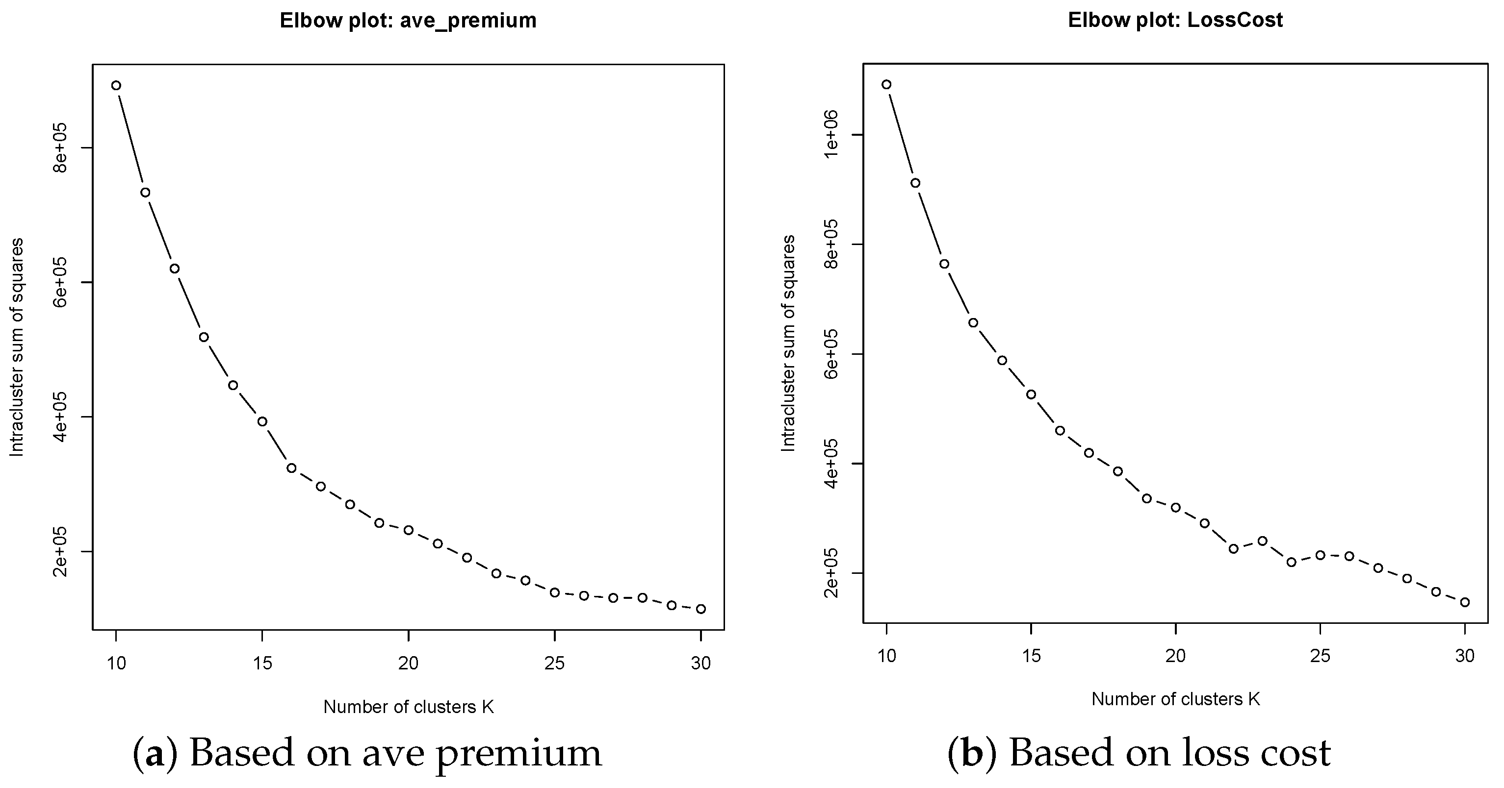
The hierarchical clustering method we have utilized in this study treats the number of clusters as a quantity to be determined before the algorithm proceeds. Some guidance is offered in Chavent et al. (2018): “According to the dendrogram, the user can select an appropriate number of clusters K with their favorite rule”. We have opted to set (K = 15) for this study, which is justified by an application of the elbow method. This result was reported in Figure 1. Hierarchical clustering fixes K throughout the study; therefore, the K represents regular behaviour of risk territories in Ontario. For purposes of evaluating the impact of the pandemic, it is sufficient to consider data before 2020—i.e., data that reflects pre-pandemic behaviour. For each of the four loss metrics—loss cost, claim severity, claim frequency, average premium—we collected the dendrograms used to create reference clusters. Due to the complexity of the data, it is not feasible to suggest a value for K by inspecting the dendrograms. We instead use the elbow method; creating the corresponding elbow plot for every loss metric confirms that () is an appropriate choice for the study.
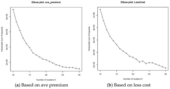
Figure 1.
The plot illustrating the relationship between the sum of squares within clusters and the number of clusters, comparing results from studies based on average premiums and loss costs.
3.3. Unified Spatial Clustering of Insurance Loss Metrics
One of the challenges in using spatial clustering for data visualization or grouping lies in the inconsistency of group labeling, particularly when dealing with data spanning multiple reporting years. The clustering process involves utilizing data from individual half-years, each corresponding to a specific reporting period. Our proposed approach begins with establishing a reference clustering, which entails defining a fixed set of groupings based on intervals of loss metrics. Subsequently, other clusters are generated by mapping the data to these pre-defined groups with assigned labels. This unified spatial clustering methodology can be likened to classifying spatial units based on training from older accident year loss data, resulting in a sub-optimal clustering of newer accident year loss data. The proposed clustering procedure and data visualization is made up of four main steps, discussed below. We take information from the pre-pandemic period as reference points and conduct clustering thereafter to produce results for each loss metric we considered, separated by major insurance coverages.
Input Data Matrices for Pre-Pandemic
We first create the necessary input data files representing pre-pandemic information about the risk territories in Ontario. As seen later when unifying the clusters, this will inform the choice of boundary points within the range of the chosen loss metrics. For each run, we choose a reporting year and a single loss metric. For every FSA, we take its all available half-year observations. These observations are formed as input data for computing the dissimilarity matrix . For instance, for reporting year 2019, the data will consist of accident year data from 2015 to 2019, and each accident year contains two half-years of data. This step of clustering pre-pandemic serves as an initial step to prepare the reference grouping for the clustering of more recent accident years, and it consists of the following eight procedures:
- Import raw data: Loss metrics by FSA for all reporting years and the FSA polygons of Ontario, which are available publicly through R packages or the Canadian statistics platform.
- Prepare clustering:
- (a)
- Select the data file with reporting year 2019 to serve as a reference point.
- (b)
- Select the major coverage type to subset by—AB, CL, TPL.
- (c)
- Select a single loss metric—either average premiums, loss cost, claim severity, or claim frequency (we choose AB and loss cost for the ease of discussion later on).
- (d)
- Create a summary data frame giving a loss metric for each FSA and each coverage.
- (e)
- Join the FSA polygons data to the summary data frame , while retaining polygons from excluded FSAs in a separate data frame .
- Create dissimilarity matrix :
- (a)
- Produce a data frame with FSA as rows and half-year as columns, giving a ten-dimensional vector for every column
- (b)
- Compute the corresponding Euclidean distance matrix
- (c)
- Normalize the dissimilarity matrix by taking
- Create dissimilarity matrix :
- (a)
- Switch off spherical geometry. This is because the imported polygons are planar.
- (b)
- Create and normalize following the procedure outlined in Chavent et al. (2018)
- Choose and fix the number of clusters K a priori and mixing parameter using a normalized plot showing explained inertia for and . We choose and in this work after careful tuning of parameters.
- Execute clustering and create a data frame assigning every FSA to a cluster.
- Find the average loss metric for each cluster, and relabel each cluster in order of average loss metric, with 1 corresponding to the cluster with highest average loss metric. Output a data frame with each FSA assigned.
- Join to and export the results.
After this initial step, we should end up with a total of 16 data frames corresponding to the major coverage type subsetting and loss metric, each containing information from the reporting year of 2019. The following second step is then taken to prepare datasets for further analysis:
Step 2: Create datasets containing ‘local’ clusters for data subsetted by major coverage type and half-year. These will be used for modeling, and act as intermediary results for data visualization.
- Choose a loss metric, major coverage type, and half-year.
- Filter the data by major coverage type and half-year.
- Match the FSA polygon information with the data of each FSA, giving the data frame
- Create and normalize by finding the distance matrix of the given loss metric column of
- Create and normalize following the procedure outlined in Chavent et al. (2018)
- Execute clustering command and create a data frame assigning every FSA to a cluster.
- Find the average loss cost for each cluster, and relabel each cluster in order of average loss cost, with 1 corresponding to the cluster with highest average loss cost. Output a data frame with each FSA assigned.
- Join to and export the results.
Repeating for all loss metrics, major coverage types and accident half years, we should create 256 datasets in total. We reinforce that for modeling purposes, this second step is sufficient to ensure a unified data grouping; the other steps only apply for data visualization.
Step 3: Unify clusters across all accident half-years data. The input files are the datasets created in step 2, and the datasets in step 1 are used for unification as reference points.
- Select a loss metric and obtain the respective four data frames giving prior clusters, produced in step 1.
- Using spatial clustering, group each data frame by cluster.
- Maps a value for the average loss metric to one of the K unified clusters. The input is the within-cluster average loss metric for a local cluster, as well as the major coverage sub-setting type:
- (a)
- Choose major coverage type and the corresponding summary data frame
- (b)
- For all i in 1 to K:
- Compare the input average of loss metrics to the average of cluster i
- If the input average is greater:
- Return cluster i
- Exit function
- Otherwise continue to
- (c)
- If the input average has still not been assigned for any cluster after iterating through the whole for loop (i.e., the input average is smaller than all of the prior cluster averages) then return cluster K
Now, we have the machinery required to place all local clusters across different half-years onto the same frame of reference. Unifying the clusters in this way allows for meaningful data visualization throughout the course of the data reporting periods. - Take all of the datasets with local clusters produced in Step 2, then for all datasets of the chosen loss metric:
- (a)
- Find the major coverage type that the dataset gives information for
- (b)
- Calculate within-cluster averages for every cluster and join the averages to each observation
- (c)
- Map each observation to the new clusters
- (d)
- Export the dataset with the polygons as well as the new clusters
Finally, with the unified clusters, we can create the maps for each loss metric, major coverage type and half year. This is achieved using the ggplot R statistical package, where the visual aspects of the plot can be customized.
This work uses hierarchical clustering for unifying clusters for multiple accident years data. Hierarchical clustering offers significant advantages for spatial clustering in risk modeling and territory design (Xie 2019; Zhang et al. 2023), primarily due to its ability to consider the geographical relationships between FSAs. The method’s flexibility in handling varying levels of granularity allows for the identification of nested spatial patterns and insights into how smaller regions aggregate into larger clusters, enhancing the precision of risk assessments. Additionally, hierarchical clustering can visually represent the clustering process through dendrograms, facilitating a deeper understanding of spatial relationships. However, its computational intensity can be a barrier, especially with large datasets, potentially leading to longer processing times and the need for substantial computational resources. Another challenge lies in the subjectivity of determining the optimal number of clusters, which can affect the consistency and reliability of the clustering outcomes. Despite these barriers, the method’s capability to capture and illustrate complex spatial dependencies makes it a valuable tool in refining risk models and designing more effective territories.
3.4. Modeling Loss Metrics Using Spatial Clusters
Our primary objective in this study is to consolidate spatial clusters when analyzing data spanning multiple accident years. For each year’s data, we generate labeled clusters. These clusters, along with accident half-years, are utilized as covariates in a Generalized Linear Model (GLM). Applying various error distribution functions and identity link functions, we model loss metrics, such as loss cost and average premium, using GLM. This modeling approach facilitates the estimation of cluster effects and accident half-year effects for each factor level. By employing GLM, we can quantify the fixed effects attributed to cluster and accident half-year factors, thereby providing insights into their respective impacts on the studied metrics. This modeling procedure will be applied by major coverage types and by different response variables. However, the model covariates remain the same for all models.
3.5. Addressing Potential Collinearity of Variables
We briefly address the possibility of dependence on accident half-year during the process of unifying clusters for visualization. We have used the chi-square test for independence on the datasets after cluster unification. The null hypothesis is that the variables of accident half-year and unified cluster are related, and the alternative hypothesis is that the variables are not dependent. For every loss metric and major coverage type, the chi-square test was carried out on the dataset with observations clustered according to our unified reference clustering and across all 16 accident half-year periods. In all cases, we found that the p-value was negligibly small; in particular, ). Hence, we reject at all levels of confidence. Therefore, in the GLM, we did not consider the interactions between clusters and accident years.
4. Results
In this section, we present our findings and their analysis based on the loss data outlined in Section 3. Through a thorough examination of spatial patterns and taking into account the number of statistical territories utilized in Ontario (comprising 19 statistical territories, some with limited credibility due to smaller risk exposures), we have opted to use a total of 15 clusters for this study. The selection of is theoretically justified by the elbow method. This predetermined number of clusters is selected to navigate the complexities and challenges associated with justifying optimality from a practical standpoint. It also aims for the consistency of practical use in the context of statistical grouping of basic rating units based on insurance loss. Moreover, our primary objective in this research is to introduce a unified clustering approach capable of effectively handling multiple sets of accident data over half-year periods, facilitating pattern comparisons.
Table 1 summarizes the ranges of loss metrics intervals linked with unified clusters, separated by major coverages. These intervals serve as benchmarks for clustering loss data. They can be treated as cluster labels denoting the extent of considered loss metrics. We can not go beyond 15 for the number of clusters as some clusters we produced have narrow intervals, leading to a limited number of FSAs to be included in the unified clustering step. Clustering other loss data would thus involve classifying them into one of these labels derived from pre-pandemic data periods to form the clusters. Therefore, one can think of this process as a training process for the purpose of defining clusters, and the spatial clustering of other accident years becomes a test process.

Table 1.
Interval for each unified cluster, respectively for Claim Frequency, Claim Severity, Loss Cost, and Average Premium by major coverages AB, CL, and TPL.
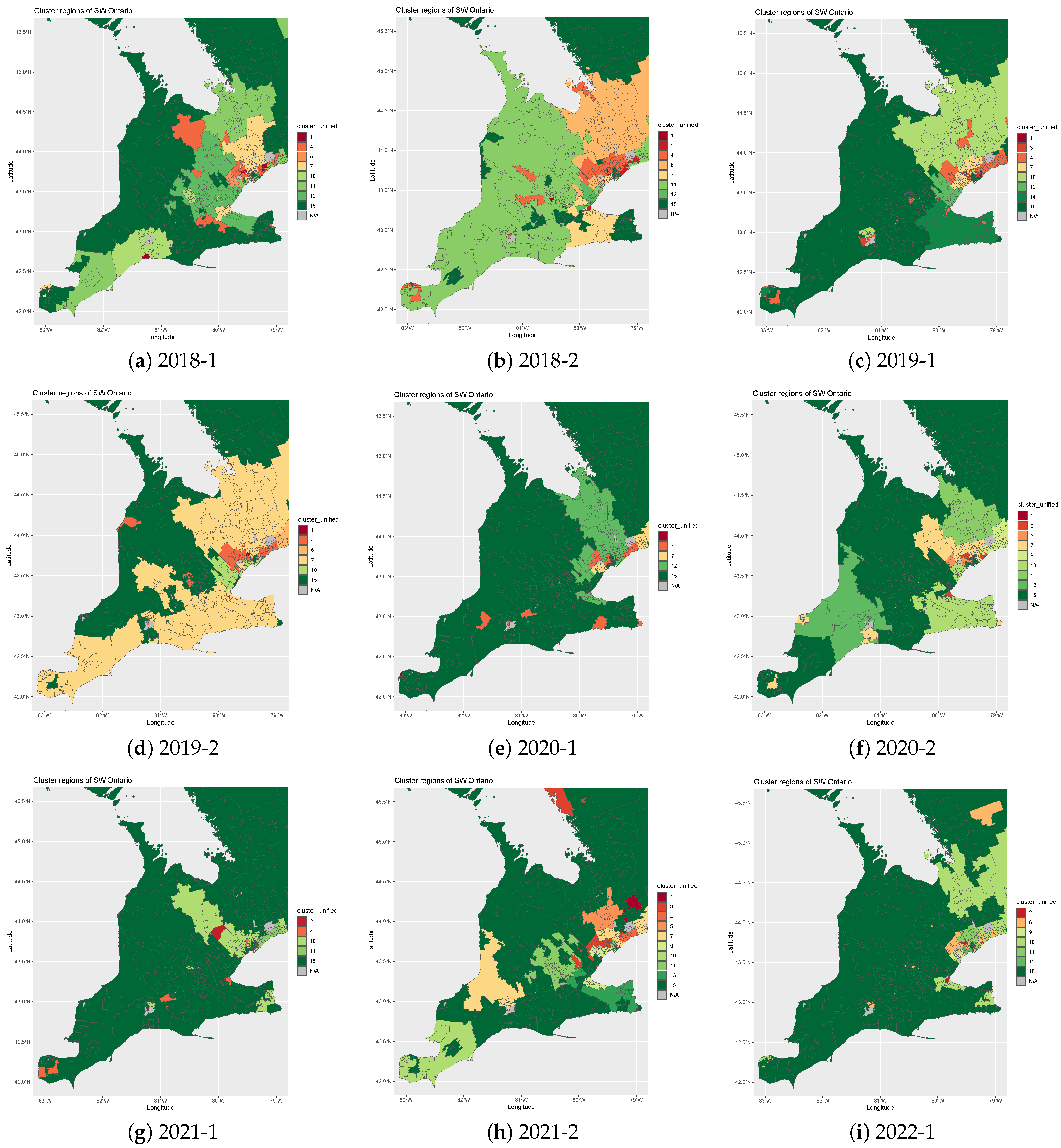
Figure 2 and Figure 3 exhibit the temporal evolution of claim severity and loss cost of AB coverage across southern Ontario from 2018 to 2022, utilizing the proposed unified spatial clustering methodology. Analyzing the AB coverage pattern in highly economically developed regions, where a substantial number of vehicles are present, offers valuable insights into the macroscopic trends of auto insurance. This facet stands as a significant impact of auto insurance coverage, shedding light on broader patterns and behaviours within these regions. It is noteworthy that the visualization results of claim severity or loss cost are based on benchmarked intervals derived from 2017 accident year data. Consequently, these temporal maps display the clustering outcomes against pre-defined labels, enabling direct comparability facilitated by the unification process.
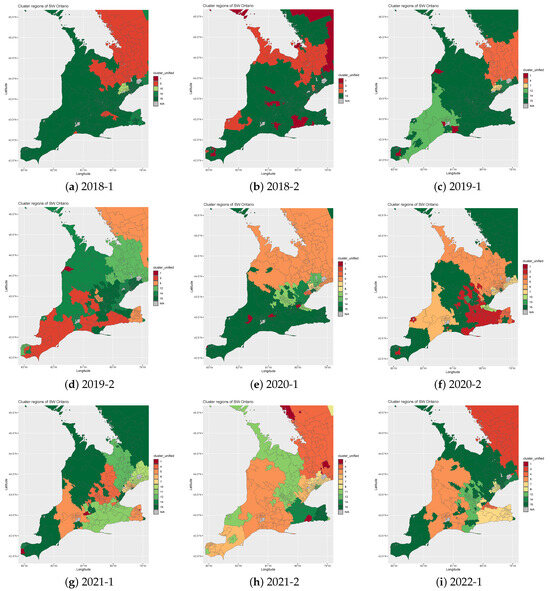
Figure 2.
The time evolutionary maps of claim severity at FSA level for AB coverage in southern Ontario, Canada from 2018-1 to 2022-1.

Figure 3.
The time evolutionary maps of loss cost at FSA level for AB coverage in southern Ontario, Canada from 2018-1 to 2022-1.
Upon examining these spatial clustering results, several interesting dynamics emerge. Firstly, there appears to be a high degree of reduction in claim severity, particularly evident beyond the Greater Toronto Area. This reduction suggests potential shifts in driving behaviors, regional infrastructure changes, or other underlying factors warranting further investigation. Moreover, the observed reduction in loss cost during the COVID-19 pandemic receives further validation through the spatial clustering analysis depicted in Figure 3. This provides some statistical evidence for the broader trend of decreased vehicular activity and subsequent impact on insurance claims and associated loss costs during periods of restricted mobility. In essence, these findings underscore the utility of unified spatial clustering techniques in uncovering meaningful insights from temporal datasets. They not only highlight the dynamic nature of risk profiles within southern Ontario but also emphasize the importance of adaptive methodologies in understanding spatial loss patterns over time.
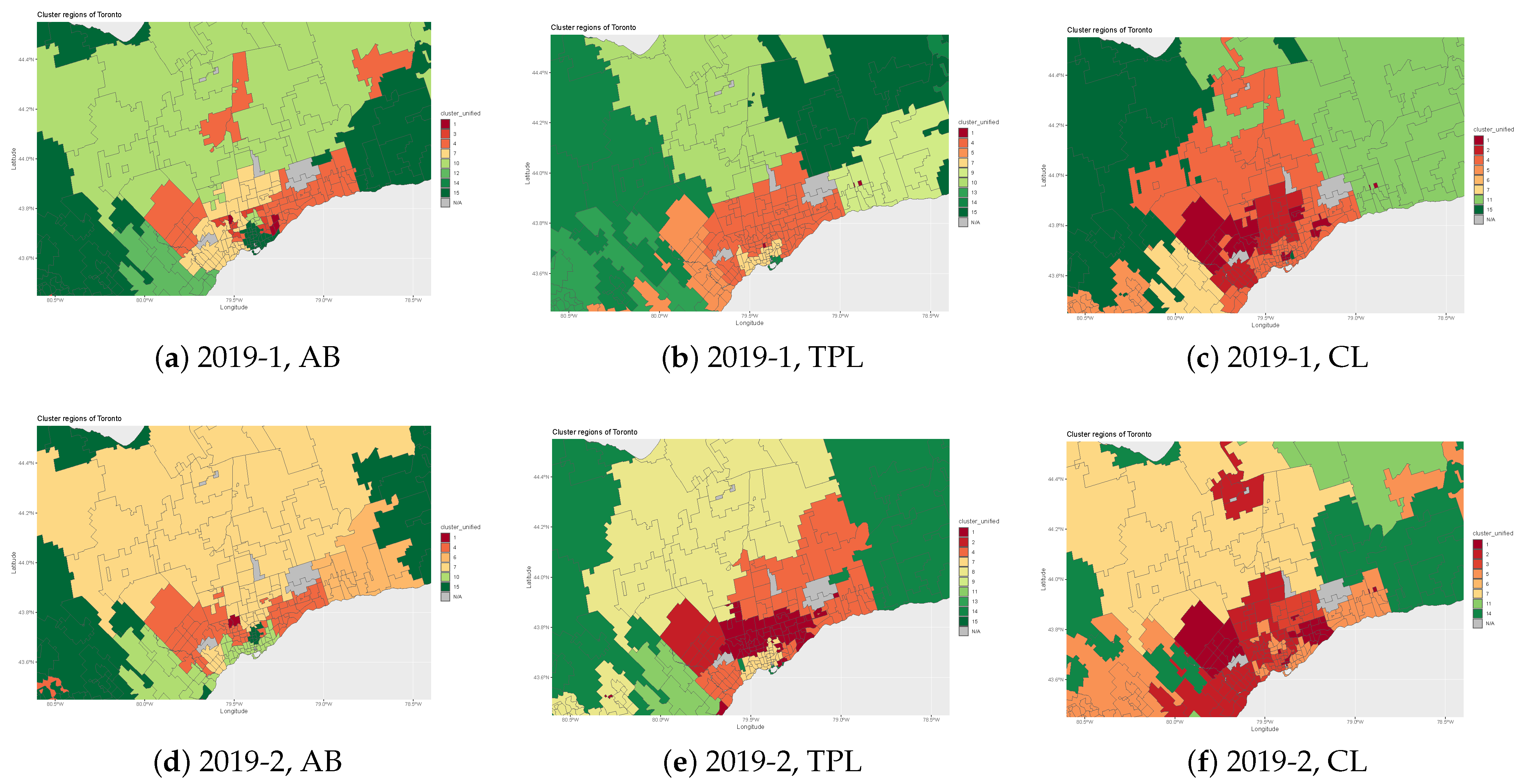
To gain a deeper understanding into the trends of insurance losses across various major coverages, we explore the patterns within the Greater Toronto Area both pre- and post-COVID-19 pandemic. This microscopic analysis would provide us significant insights of loss patterns for a major metropolitan city. Our analysis focuses on loss cost, and the findings are presented in Figure 4 and Figure 5. By comparing the loss patterns between pre-pandemic and after-pandemic, one can observe the significant reduction in loss cost in the downtown Toronto area. This is mainly contributed by a reduction in claim frequency as our study shows no significant change in claim severity. The claim severity slightly increased after the pandemic, which may be due to the global crisis of the supply chain that causes a higher expense settling claims. We also observe that CL coverage is most affected by the pandemic, while the AB coverage is least influenced. This may be because the loss cost associated with AB coverage is more related to medical costs, while CL coverage is mainly the cost associated with physical damage to vehicles.
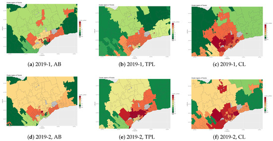
Figure 4.
The loss cost map for Greater Toronto Area at FSA level for right before COVID-19 pandemic (2020 accident year) by coverage.
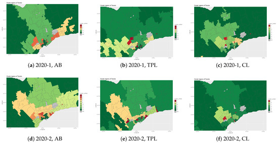
Figure 5.
The loss cost map for Greater Toronto Area at FSA level for right after COVID-19 pandemic (i.e., 2020 accident year) by coverage.
In this work, a major effort is to model loss costs and average premium charges for unified clusters so that the territory risk can be quantified. The results are reported in Table 2, Table 3, Table 4, Table 5, Table 6 and Table 7, respectively, for AB, TPL, and CL. Our first observation is the consistency of model coefficients between average premiums and loss costs within the coverage. Overall, within the same coverage, average premiums have a better distribution fitting performance, which leads to a higher adjusted and lower AIC value when compared to loss cost. This is due to the adjustment of premium charges that depart from the actual loss cost in order to overall optimize the insurance pricing, which will benefit the underwriting process. The second observation is that the model fitting performance for average premiums and loss cost by coverage depends on the error distribution function used in GLM. For instance, inverse Gaussian distribution leads to the best adjusted for average premium data that is associated with CL coverage while the Poisson error function works the best for TPL coverage. However, the model fitting performance does not greatly depend on the error distribution used for TPL coverage. For loss cost data, the normal and Poisson error functions significantly outperform other choices. Additionally, the model fitting performance appears to be more influenced by the choice of error functions for AB and TPL in modeling loss cost.
Table 2.
The model coefficients and goodness of fit measures for modeling AB coverage Average Premium data under different choices of error distributions.
Table 3.
The model coefficients and goodness of fit measures for modeling TPL coverage Average Premium data under different choices of error distributions.
Table 4.
The model coefficients and goodness of fit measures for modeling CL coverage Average Premium data under different choices of error distributions.
Table 5.
The model coefficients and goodness of fit measures for modeling AB coverage loss cost data under different choices of error distributions.
Table 6.
The model coefficients and goodness of fit measures for modeling CL coverage loss cost data under different choices of error distributions.
Table 7.
The model coefficients and goodness of fit measures for modeling TPL coverage loss cost data under different choices of error distributions.
The unification of spatial clusters enables the ordering of territory risk and makes the comparison of estimated coefficients associated with each cluster easier. From the results, we observe that data variation is mainly explained by spatial clusters, rather than the accident half-year variable. This implies that territory is the dominant factor in pricing and affecting loss cost values. We can also see a significant drop in the loss cost for both coverages during the pandemic, but their values increased again after the pandemic. However, we did not see clearly that the average premium charged during the pandemic decreased significantly. Instead, we observe a significant increase in average premiums for CL coverage.
This work builds upon the research conducted in Xie and Gan (2023), which employed fuzzy clustering to create clusters. Both fuzzy clustering and spatial clustering consider neighboring elements; however, spatial clustering primarily focuses on spatial domain relationships. A key limitation of fuzzy clustering is that it applies to a single reporting year and averages losses across different accident years. In contrast, unified spatial clustering addresses multiple accident year datasets simultaneously.
5. Conclusions
In auto insurance, complexities arise when clustering multiple accident years of claim data, necessitating specialized methodologies. Through such analyses, insurers and regulators gain valuable insights into trends and levels of territory risk. For instance, the observed reduction in loss costs during the pandemic period, attributed to decreased vehicular activity due to mobility restrictions, underscores the importance of understanding and adapting to fluctuating risk landscapes. These insights are crucial for regulators when approving insurance rate changes to reflect the evolving risk profiles of insurance companies.
A microscopic analysis of the Greater Toronto Area reveals localized trends in loss patterns. Post-pandemic, a notable decrease in loss costs, particularly in downtown Toronto, is primarily driven by reduced claim frequency rather than claim severity. This suggests shifts in driving behaviors or other urban-specific factors, necessitating regulatory considerations. The analysis also highlights coverage-specific impacts, with differential effects observed for various coverage types, such as CL and AB. While AB coverage experiences relatively minor effects, CL coverage sees more significant reductions, likely due to differences in the nature of claims associated with each coverage type. Such insights underscore the importance of considering coverage-specific factors in rate regulation decisions. Moreover, modeling loss costs and average premium charges for unified clusters helps quantify territory risk. The defined clusters with fixed labels replace the territories represented by FSA, enabling overall control of all regions in terms of their risk levels. The dominance of spatial clusters in explaining data variation highlights the significance of territorial risk in pricing and regulating auto insurance rates.
In essence, the findings demonstrate the critical role of advanced analytical techniques in shaping auto insurance rate regulation policies. By incorporating insights obtained from spatial clustering and temporal trend analysis, regulators can better adapt to evolving risk landscapes, ensuring the sustainability and fairness of the insurance market. Future work will focus on further investigating the optimal design of clusters and their impact on modeling outcomes using goodness-of-fit measures such as Adjusted . Additionally, modeling loss costs using the Tweedy family as error distribution functions is a valuable avenue for practical improvements in auto insurance pricing and rate regulation.
For insurers and regulatory authorities, the practical implications of using spatial clustering to investigate insurance loss patterns are profound. Insurers can develop more accurate risk profiles, leading to better pricing strategies and more targeted marketing efforts. Regulatory authorities can ensure fairer pricing and more effective oversight by understanding regional risk variations. For policyholders, particularly drivers in urban environments, this could translate to more equitable insurance premiums based on precise risk assessments, potentially influencing driving behaviors to lower risks and premiums. In urban settings, factors like traffic density, road conditions, and crime rates can be better integrated into risk models, providing a comprehensive view of insurance needs.
Scientifically, spatial clustering opens new avenues for researchers interested in urban planning, public policy, and environmental studies. Researchers can leverage this method to uncover spatial patterns that inform urban development and resource allocation. Future research will explore various approaches to spatial clustering, including integrating data from multiple accident years to ensure consistent labeling across different years. Additionally, comparative data analyses for each accident year and advancements in data visualization techniques will be pursued to effectively handle multiple datasets.
Author Contributions
Conceptualization, S.X.; methodology, S.X.; software, S.X; validation, S.X and N.H.; formal analysis, S.X. and N.H.; investigation, S.X. and N.H.; resources, S.X.; data curation, S.X.; writing—original draft preparation, S.X.; writing—review and editing, S.X. and N.H.; visualization, N.H. All authors have read and agreed to the published version of the manuscript.
Funding
There is no funding support for this research project.
Data Availability Statement
The data belong to the regulator and are subject to approval by the regulator.
Conflicts of Interest
The authors declare no conflicts of interest.
References
- Andrews, Marcus R., Kosuke Tamura, Janae N. Best, Joniqua N. Ceasar, Kaylin G. Batey, Troy A. Kearse, Jr., Lavell V. Allen, III, Yvonne Baumer, Billy S. Collins, Valerie M. Mitchell, and et al. 2021. Spatial clustering of county-level COVID-19 rates in the US. International Journal of Environmental Research and Public Health 18: 12170. [Google Scholar] [CrossRef]
- Aslam, Faheem, Ahmed Imran Hunjra, Zied Ftiti, Wael Louhichi, and Tahira Shams. 2022. Insurance fraud detection: Evidence from artificial intelligence and machine learning. Research in International Business and Finance 62: 101744. [Google Scholar] [CrossRef]
- Chavent, Marie, Vanessa Kuentz-Simonet, Amaury Labenne, and Jérôme Saracco. 2018. ClustGeo: An R package for hierarchical clustering with spatial constraints. Computational Statistics 33: 1799–822. [Google Scholar] [CrossRef]
- Chowdhury, Subrata, P. Mayilvahanan, and Ramya Govindaraj. 2022. Optimal feature extraction and classification-oriented medical insurance prediction model: Machine learning integrated with the internet of things. International Journal of Computers and Applications 44: 278–90. [Google Scholar] [CrossRef]
- Cummins, Enda J., Patrick M. Grace, Kevin P. McDonnell, Shane M. Ward, and D. John Fry. 2001. Predictive modelling and risk assessment of BSE: A review. Journal of Risk Research 4: 251–74. [Google Scholar] [CrossRef]
- Hussain, Walayat, Jose M. Merigó, Muhammad Raheel Raza, and Honghao Gao. 2022. A new QoS prediction model using hybrid IOWA-ANFIS with fuzzy C-means, subtractive clustering and grid partitioning. Information Sciences 584: 280–300. [Google Scholar] [CrossRef]
- Inostroza, Luis, Rolf Baur, and Elmar Csaplovics. 2013. Urban sprawl and fragmentation in Latin America: A dynamic quantification and characterization of spatial patterns. Journal of Environmental Management 115: 87–97. [Google Scholar] [CrossRef]
- Kulldorff, Martin. 1994. Spatial disease clusters: Detection and inference. Statistics in Medicine 13: 1–12. [Google Scholar] [CrossRef]
- La Bella, Alessio, Pascal Klaus, Giancarlo Ferrari-Trecate, and Riccardo Scattolini. 2022. Supervised model predictive control of large-scale electricity networks via clustering methods. Optimal Control Applications and Methods 43: 44–64. [Google Scholar] [CrossRef]
- Li, Hong, and Jianxi Su. 2022. Mitigating wildfire losses via insurance-linked securities: Modeling and risk management perspectives. Journal of Risk and Insurance 91: 383–414. [Google Scholar] [CrossRef]
- Liu, Mengyang, Mengmeng Liu, Zhiwei Li, Yingxuan Zhu, Yue Liu, Xiaonan Wang, Lixin Tao, and Xiuhua Guo. 2021. The spatial clustering analysis of COVID-19 and its associated factors in mainland China at the prefecture level. Science of the Total Environment 777: 145992. [Google Scholar] [CrossRef]
- Mennis, Jeremy, and Philip Harris. 2013. Spatial contagion of male juvenile drug offending across socioeconomically homogeneous neighborhoods. In Crime Modeling and Mapping Using Geospatial Technologies. Dordrecht: Springer, pp. 227–48. [Google Scholar]
- Patil, G. P., R. Modarres, W. L. Myers, and P. Patankar. 2006. Spatially constrained clustering and upper level set scan hotspot detection in surveillance geoinformatics. Environmental and Ecological Statistics 13: 365–77. [Google Scholar] [CrossRef]
- Ramachandra, T. V., Bharath H. Aithal, and Durgappa D. Sanna. 2012. Insights to urban dynamics through landscape spatial pattern analysis. International Journal of Applied Earth Observation and Geoinformation 18: 329–43. [Google Scholar]
- Ramos, Antônio Carlos Vieira, Mellina Yamamura, Luiz Henrique Arroyo, Marcela Paschoal Popolin, Francisco Chiaravalloti Neto, Pedro Fredemir Palha, Severina Alice da Costa Uchoa, Flávia Meneguetti Pieri, Ione Carvalho Pinto, Regina Célia Fiorati, and et al. 2017. Spatial clustering and local risk of leprosy in São Paulo, Brazil. PLoS Neglected Tropical Diseases 11: e0005381. [Google Scholar] [CrossRef] [PubMed]
- Seresht, Nima Gerami, Rodolfo Lourenzutti, and Aminah Robinson Fayek. 2020. A fuzzy clustering algorithm for developing predictive models in construction applications. Applied Soft Computing 96: 106679. [Google Scholar] [CrossRef]
- Wang, Rina Meng-Jie. 2023. The Application of Categorical Embedding and Spatial-Constraint Clustering Methods in Nested GLM Model. Master’s thesis, Simon Fraser University, Burnaby, BC, Canada. [Google Scholar]
- Wang, Shaobin, and Jun Wu. 2020. Spatial heterogeneity of the associations of economic and health care factors with infant mortality in China using geographically weighted regression and spatial clustering. Social Science & Medicine 263: 113287. [Google Scholar]
- Xie, Shengkun. 2019. Defining geographical rating territories in auto insurance regulation by spatially constrained clustering. Risks 7: 42. [Google Scholar] [CrossRef]
- Xie, Shengkun, and Chong Gan. 2023. Estimating Territory Risk Relativity Using Generalized Linear Mixed Models and Fuzzy C-Means Clustering. Risks 11: 99. [Google Scholar] [CrossRef]
- Xie, Shengkun, Anna T. Lawniczak, and Zizhen Wang. 2017. Spatially Constrained Clustering to Define Geographical Rating Territories. Paper presented at International Conference on Pattern Recognition Applications and Methods, Porto, Portugal, February 24–26; Setúbal: SCITEPRESS, vol. 2, pp. 82–88. [Google Scholar]
- Zhang, Hao, Zhi-fang Qi, Xin-yue Ye, Yuan-bin Cai, Wei-chun Ma, and Ming-nan Chen. 2013. Analysis of land use/land cover change, population shift, and their effects on spatiotemporal patterns of urban heat islands in metropolitan Shanghai, China. Applied Geography 44: 121–33. [Google Scholar] [CrossRef]
- Zhang, Ying, Semu Moges, and Paul Block. 2016. Optimal cluster analysis for objective regionalization of seasonal precipitation in regions of high spatial–temporal variability: Application to Western Ethiopia. Journal of Climate 29: 3697–717. [Google Scholar] [CrossRef]
- Zhang, Zuo, Yuqian Dou, Xiaoge Liu, and Zhe Gong. 2023. Multi-hierarchical spatial clustering for characteristic towns in China: An Orange-based framework to integrate GIS and Geodetector. Journal of Geographical Sciences 33: 618–38. [Google Scholar] [CrossRef]
- Zhu, Jie, Jiazhu Zheng, Shaoning Di, Shu Wang, and Jing Yang. 2020. A dual spatial clustering method in the presence of heterogeneity and noise. Transactions in GIS 24: 1799–826. [Google Scholar] [CrossRef]


Disclaimer/Publisher’s Note: The statements, opinions and data contained in all publications are solely those of the individual author(s) and contributor(s) and not of MDPI and/or the editor(s). MDPI and/or the editor(s) disclaim responsibility for any injury to people or property resulting from any ideas, methods, instructions or products referred to in the content. |
© 2024 by the authors. Licensee MDPI, Basel, Switzerland. This article is an open access article distributed under the terms and conditions of the Creative Commons Attribution (CC BY) license (https://creativecommons.org/licenses/by/4.0/).