A Hypothesis Test for the Long-Term Calibration in Rating Systems with Overlapping Time Windows

Abstract

We present a statistical test for the long-term calibration in rating systems that can deal with overlapping time windows as required by the guidelines of the European Banking Authority (EBA), which apply to major financial institutions in the European System. In accordance with regulation, rating systems are to be calibrated and validated with respect to the long-run default rate. The consideration of one-year default rates on a quarterly basis leads to correlation effects which drastically influence the variance of the long-run default rate. In a first step, we show that the long-run default rate is approximately normally distributed. We then perform a detailed analysis of the correlation effects caused by the overlapping time windows and solve the problem of an unknown distribution of default probabilities.

1. Introduction

Financial institutions use statistical models to estimate the default risk of obligors in order to manage credit risks. According to Basel II, banks are allowed to estimate risk parameters that are used to calculate regulatory capital with their own models. The legal framework for the use of such models in the internal ratings-based (IRB) approach is regulated in the Capital Requirements Regulation (CRR), see CRR (2013). In Cucinelli et al. (2018), the authors conclude that the IRB regulatory framework has promoted stronger risk management practices and strengthened banks’ overall resilience. The CRR imposes specific requirements for the models, e.g., that “institutions shall estimate PDs [probabilities of default] by obligor grade from long run averages of one-year default rates”, see Article 180. In 2017, the European banking authority published the “guidelines on PD estimation, LGD [loss given default] estimation and the treatment of defaulted exposures” (EBA-GL) specifying the CRR requirement, see EBA GL (2017). Paragraph 81 EBA-GL states that “institutions should calculate the observed average default rates as the arithmetic average of all one year default rates”. This requirement was additionally specified in EBA (2016) and ECB (2024). Here, the observed one-year default rate at a given reference date is defined as the percentage of defaulters in the 12-month period after the reference date, so that the observed long-run average default rate depends on the choice of the reference dates. Paragraph 80 EBA-GL allows institutions to choose “between an approach based on overlapping and an approach based on non-overlapping one-year time windows”. Overlapping one-year time windows occur when the time interval between two reference dates is less than one year. Due to computational simplicity, it is of course convenient to continue working with non-overlapping time windows and appropriately adjust the long-term default rate. In many cases, these types of adjustments are rather on the conservative side, see, e.g., Jing et al. (2008) for an empirical study and Li (2016); Zhou (2001) for theoretical analyses in the context of asset correlation. We also refer to Caprioli et al. (2023) for a sensitivity analysis of credit portfolio value at risk with respect to asset correlations.

On the other hand, the approach, using overlapping time windows, provides more information on defaults due to both potential short-term contracts that cannot be observed during one-year periods and possible variations between average default rates using non-overlapping time windows on different reference dates. Especially in such constellations, it is “the ECB’s understanding that overlapping one-year time windows should preferably be used”, see ECB (2024). For this reason, dealing with overlapping time windows is relevant for all major banks in the eurozone using the IRB approach. Furthermore it is favored by most financial institutions that handle portfolios with only few observed defaults, where the estimation and validation of PDs are particularly challenging, cf. Caprioli et al. (2023); Pluto and Tasche (2011); Tasche (2013). Another advantage of this approach lies in the fact that the bias caused by a specific choice of reference dates can be reduced, e.g., when calculating the long-run average default rate as the arithmetic mean of the one-year default rates on a quarterly basis.

Paragraph 87 EBA-GL requires institutions to use a statistical test of calibration at the level of rating grades and for certain portfolios. Classically, the literature dealing with calibration tests assumes a binomially distributed default rate, see, e.g., Deutsche Bundesbank (2003) and Tasche (2008) for a discussion of different hypothesis tests in this context. We also refer to Coppens et al. (2016) for the consideration of different PDs within the same rating grade and Blochwitz et al. (2004, 2006) for a modified binomial test accounting correlated defaults. However, when considering overlapping time windows, the assumption of a binomial distribution can no longer be maintained. For an overview of existing statistical tests, including a hybrid test that represents a combination of exact and approximate testing procedures, we refer to Aussenegg et al. (2011).

More generally, Monte Carlo methods can be used to construct tests for distributions that cannot be determined analytically. For the use of Monte Carlo methods, precise knowledge of the distribution of the probabilities of default within the portfolio is essential. However, in our case, these probabilities are unknown and estimated by the underlying model so they cannot be used to determine the test statistic. On the other hand, analytical tests are desirable since they satisfy requirements such as replicability and reproducibility. We refer to Blöchlinger (2012, 2017) for hypothesis tests in analytic form that take into account correlation effects, replacing the i.i.d. assumption by a conditional i.i.d. assumption. In this context, we also refer to Tasche (2003) for a one-observation-based inference on the adequacy of probability of default forecasts with dependent default events.

In this paper, we therefore present a statistical test that can be used to verify supervisory calibration requirements in the case of overlapping time windows. A major challenge lies in the analysis of the correlation effects that are caused by the overlapping time windows. On the level of individual ratings grades, the variance of the test statistic is already determined by the null hypothesis. This, however, is not the case on a portfolio level, which is why we focus in great detail on a conservative estimate for the variance by solving a related minimization problem. We then present a conservative calibration test that can deal with the unknown variance in the test statistic.

The rest of the paper is structured as follows. In Section 2.1, we introduce the terminology and notation for the formulation of the hypothesis test in Section 2.2. In Section 2.3, we show that the long-run default rate is approximately normally distributed with respect to random effects in default realization. Thereafter, we focus on the analysis of the correlation effects that arise due to the overlapping time periods in Section 2.4 and Section 2.5. Taking these correlation effects into account is essential for determining the variance of the long-run default rate, see Section 2.6. In Section 3 we formulate the hypothesis test in detail, first at the level of individual rating grades, cf. Section 3.1 and then at portfolio level, cf. Section 3.2. We conclude with a discussion on the parameters of the test and further considerations in Section 4. A closed form solution to the minimization problem related to the estimation of the variance is derived in Appendix A. In Appendix B, we propose an alternative way to estimate the variance without solving an optimization problem.

2. Setup and Preliminaries

2.1. Setup and Notation

In this section, we introduce the terminology and notation used in this paper and give a formal description of the statistical test that is studied in this work. We begin with the general setup by considering the default state of an individual obligor. Throughout, a default state over a one-year time horizon is described by a Bernoulli-distributed random variable $x\sim B\left(1,p\right)$, where

$$p\in \left\{{\mathrm{PD}}_1,\dots ,{\mathrm{PD}}_m\right\},$$

$m\in \mathbb{N}$, and $0<{\mathrm{PD}}_1<\dots <{\mathrm{PD}}_m<1$ are the default probabilities of the rating grades in the underlying master scale. In the following, we also use the notations ${\mathrm{PD}}_{min}$ and ${\mathrm{PD}}_{max}$ for the default probabilities ${\mathrm{PD}}_1$ and ${\mathrm{PD}}_m$, respectively.

Next, we introduce the long-run default rate for a given history of reference dates ${\mathrm{RD}}_1<\dots <{\mathrm{RD}}_N$ with $N\in \mathbb{N}$. For all $t=1,\dots ,N$, we are given a number $n_t\in {\mathbb{N}}_0$ of customers within the portfolio at the reference date ${\mathrm{RD}}_t$, and write

$$n_{min}:=min\left(\left\{n_t\right|t=1,\dots ,N\}\setminus \left\{0\right\}\right)\mathrm{and}{n}_{max}:=max\left\{n_t\right|t=1,\dots ,N\}$$

for the minimal and maximal number of existing customers at any reference date throughout the history of the portfolio, respectively. Throughout, we assume that $n_{max}\ne 0$ or, equivalently, that $n_t\ne 0$ for some $t=1,\dots ,N$.

Let $q\in \mathbb{N}$ be the number of reference dates within a one-year time horizon starting from an arbitrary reference date. To be more precise, we assume that

$${\mathrm{RD}}_{t+1}={\mathrm{RD}}_t+{\displaystyle \frac{1}{q}}\mathrm{for}\mathrm{all}t=1,\dots ,N-1.$$

According to the EBA guidelines EBA GL (2017), the long-run default rate should be computed at least on a quarterly basis, i.e., $q=4$, or on an annual basis, i.e., $q=1$, performing, however, an analysis of the possible bias that occurs due to the negligence of quarterly data. The main interest of our analysis lies in the case $q>1$ leading to correlation effects caused by overlapping time windows. For $s,t=1,\dots ,N$ with $s>t$, we define $w_{t,s}:=max\{0,{\mathrm{RD}}_t+1-{\mathrm{RD}}_s\}$ for the size of the overlap of the observation periods.

Since new customers are usually added over time and the business relationship ends for others, assign to each customer during the history of reference dates a number from 1 to $M\in \mathbb{N}$, and we define ${\Lambda }_t\subseteq \{1,..,M\}$ as the set of obligors at reference date ${\mathrm{RD}}_t$ for all $t=1,\dots ,N$. In particular, ${\bigcup }_{t=1}^N{\Lambda }_t=\{1,\dots ,M\}$, $\left|{\Lambda }_t\right|=n_t$, and $n_{max}\le M$. For $t=1,\dots ,N$, we then define the one-year default rate among the considered customers at reference date ${\mathrm{RD}}_t$ by

$$\begin{array}{c}\hfill X_t={\displaystyle \frac{1}{n_t}}\sum _{j\in {\Lambda }_t}{x}_{j,t},\end{array}$$

(1)

where $x_{t,j}\sim B(1,p_{t,j})$ is the one-year default state and $p_{t,j}\in \left\{{\mathrm{PD}}_1,\dots ,{\mathrm{PD}}_m\right\}$ the probability of default over a one-year time horizon of customer $j\in {\Lambda }_t$ at the reference date ${\mathrm{RD}}_t$. Since $n_t=0$ cannot be excluded, we use the convention ${\displaystyle \frac{0}{0}}:=0$.

The realized default rate on a reference date ${\mathrm{RD}}_t$ is denoted by ${\mathrm{DR}}_t$, i.e., ${\mathrm{DR}}_t$ is the realization of the random variable $X_t$ for $t=1,\dots ,N$. Moreover, we define

$$R_N:=\left\{t\in \{1,\dots ,N\}|n_t>0\right\}$$

as the set of indices for reference dates, where the portfolio contains at least one customer, and denote its cardinality by $R\left(N\right)$. Since we assume that $n_{max}\ne 0$, it follows that $R\left(N\right)>0$, and we define the realized long-run default rate as

$$\mathrm{LRDR}:={\displaystyle \frac{1}{R\left(N\right)}}\sum _{t=1}^N{\mathrm{DR}}_t,$$

which is a realization of the the long-run default rate

$$\begin{array}{c}\hfill Z:={\displaystyle \frac{1}{R\left(N\right)}}\sum _{t=1}^N{X}_t.\end{array}$$

(2)

We emphasize that the long-run default rate is the arithmetic mean of the one-year default rates and not the arithmetic mean of the individual default states of all customers for all reference dates, which intuition might suggest. Due to the chosen convention ${\displaystyle \frac{0}{0}}=0$, it follows that $X_t=0$ if $n_t=0$, i.e., reference dates, where the portfolio contains no customers are completely disregarded in the computation of the long-run default rate. Nevertheless, these reference dates have to be included into the timeline since they describe an overlapping period.

2.2. Formal Description of the Test

We now give an overview over the hypothesis test presented in this paper. The aim is to formulate a statistical test for comparing the realized long-run default rate $\mathrm{LRDR}$ with the estimated long-run default rate, which is called the long-run central tendency, denoted by $\mathrm{LRCT}$, both on the level of individual rating grades and on the portfolio level. In other words, $\mathrm{LRDR}$ describes the default rate that has actually occurred, while $\mathrm{LRCT}$ represents the long-run prediction from the rating model. Both $\mathrm{LRDR}$ and $\mathrm{LRCT}$ are therefore non-random. We use the random variable Z with expected value $\mu :=\mathbb{E}\left(Z\right)$ as the test statistic. Since $\mathrm{LRCT}$ is the estimated expected value of Z, i.e., $\mathrm{LRCT}=\widehat{\mu }$, we can formulate the following hypothesis test with

$$\begin{array}{cc}\hfill & \mathrm{null}\mathrm{hypothesis}{H}_0:\mu =\mathrm{LRCT}\mathrm{and}\hfill \\ \hfill & \mathrm{alternative}\mathrm{hypothesis}{H}_1:\mu \ne \mathrm{LRCT}.\hfill \end{array}$$

Based on this, we determine values $k,K\in [0,1]$ and consider the test function

$$\phi \left(z\right):=\left\{\begin{array}{cc}0,\hfill & \mathrm{if}z\in [k,K],\hfill \\ 1,\hfill & \mathrm{otherwise}.\hfill \end{array}\right.$$

(3)

If $\phi \left(\mathrm{LRDR}\right)=0$, the null hypothesis based on the available data is retained, whereas it is rejected in favor of the alternative hypothesis if $\phi \left(\mathrm{LRDR}\right)=1$. We point out that the distribution of the test statistic Z does not only depend on $\mu$ but also on other parameters that are not determined by the null hypothesis. The main focus of this paper is to postulate a distributional assumption for Z such that its distribution is determined by the null hypothesis. In this context, we first show that Z is approximately normally distributed, i.e., $Z\sim \mathcal{N}\left(\mu ,{\sigma }^2\right)$. In a second step, the focus lies on a conservative estimate for the variance ${\sigma }^2$ based on the information given by the null hypothesis. A major challenge lies in the fact that the consideration of overlapping time windows leads to unavoidable correlation effects that rule out independence assumptions on the random variables $X_1,\dots ,X_N$.

2.3. Distribution of the Long-Run Default Rate

As we have seen in the previous section, the long-run calibration test requires the formulation of a distribution assumption for the long-run default rate. However, the definition of the long-run default rate as the arithmetic mean of the one-year default rates leads to difficulties in the derivation of an analytical description of the distribution based on the Bernoulli-distributed default states of the individual obligors. The aim of this section is to show that, despite the correlation effects and the possibly varying number of obligors with different PDs at each reference date, the long-run default rate is still approximately normally distributed.

In order to simplify notation, we define $y_{t,j}:=x_{t,j}$ if $j\in {\Lambda }_t$ and $y_{t,j}:=0$ otherwise, for all $t=1,\dots ,N$. Then,

$$Z={\displaystyle \frac{1}{R\left(N\right)}}\sum _{t=1}^N{\displaystyle \frac{1}{n_t}}\sum _{j=1}^M{y}_{t,j}=\sum _{j=1}^M{Y}_j$$

with $Y_j=\sum _{t=1}^N{\displaystyle \frac{1}{R\left(N\right)}}{\displaystyle \frac{1}{n_t}}{y}_{t,j}.$

In the sequel, we will show that Z is approximately normally distributed. For this, we assume that default states of different obligors are independent of each other, from which the independence of the family ${\left(Y_j\right)}_{j=1,\dots ,M}$ follows. This assumption is standard and sufficiently conservative for the calibration of rating models.

In order to apply the Lindeberg–Feller central limit theorem (CLT), cf. (Klenke 2020, Theorem 15.44), which is a generalization of the classical CLT, we first show that the variances of the random variables ${\left(Y_j\right)}_{j=1,\dots ,M}$ cannot become arbitrarily small. In fact, by neglecting the covariance between the default states of an obligor at different reference dates,

$$\begin{array}{cc}\hfill {\sigma }^2\left(Y_j\right)& ={\displaystyle \frac{1}{R{\left(N\right)}^2}}\sum _{t=1}^N\left({\displaystyle \frac{1}{n_t^2}}{\sigma }^2\left(y_{t,j}\right)+2{\displaystyle \frac{1}{R{\left(N\right)}^2}}\sum _{s=t+1}^N{\displaystyle \frac{1}{n_t{n}_s}}\mathrm{Cov}(y_{t,j},y_{s,j})\right)\hfill \\ \hfill & \ge {\displaystyle \frac{1}{R{\left(N\right)}^2}}\sum _{t=1}^N{\displaystyle \frac{1}{n_t^2}}{\sigma }^2\left(y_{t,j}\right)\mathrm{for}\mathrm{all}j=1,\dots ,M.\hfill \end{array}$$

Note that, in the previous estimate, we have used the inequality

$$\sum _{s=t+1}^N{\displaystyle \frac{1}{n_t{n}_s}}\mathrm{Cov}(y_{t,j},y_{s,j})\ge 0,$$

which is not automatically satisfied but rather follows from Formula (5) below, which results from the additional assumptions and considerations on default states in Section 2.4. Moreover, for each obligor $j=1,\dots ,M$, there exists at least one index $t=1,\dots ,N$ with ${\sigma }^2\left(y_{t,j}\right)>0$ since ${\bigcup }_{t=1}^N{\Lambda }_t=\{1,\dots ,M\}$. Hence, for each obligor $j=1,\dots ,M$,

$${\sigma }^2\left(Y_j\right)\ge {\displaystyle \frac{1}{R\left(N\right)}}{\displaystyle \frac{1}{n_{max}^2}}\underset{k=1,\dots ,m}{min}\left\{\left({\mathrm{PD}}_k(1-{\mathrm{PD}}_k)\right)\right\}=:v_{min}.$$

Note that $v_{min}$, as defined on the right-hand side of the previous estimate, is independent of the customer $j=1,\dots ,M$ and $v_{min}>0$. Since, up to now, we only consider finitely many customers, we extend the family ${\left(Y_j\right)}_{j=1,\dots ,M}$ by a sequence of independent random variables $Y_{M+1},Y_{M+2},\dots$ with ${\sigma }^2\left(Y_j\right)\ge v_{min}$, e.g., $Y_j\sim \mathcal{N}\left({\mu }_j,v_{min}\right)$ with arbitrary drift ${\mu }_j\in (0,1)$ for $j\ge M+1$.

Now, the central limit theorem shall be applied to the family ${\left(Y_j\right)}_{j\in \mathbb{N}}$. In the classical version by Lindeberg and Lévy, the CLT states that a proper renormalization of the arithmetic mean is approximately normally distributed if the underlying sequence of random variables is independent and identically distributed. Its generalized version by Lindeberg and Feller also applies to random variables that are not identically distributed as in our case. It states that a proper renormalization of the arithmetic mean of a family of independent random variables converges in probability against a normally distributed random variable if this family satisfies the so-called Lindeberg condition, see (Klenke 2020, Definition 15.41). In our case, the Lindeberg condition applies if, for all $\epsilon >0$,

$$\underset{k\to \infty }{lim}{\displaystyle \frac{1}{s_k^2}}\sum _{j=1}^k\mathbb{E}\left({\left(Y_j-\mathbb{E}\left(Y_j\right)\right)}^2·{\mathbb{1}}_{\left\{\left|Y_j-\mathbb{E}\left(Y_j\right)\right|>\epsilon s_k\right\}}\right)=0,$$

where

$$s_k=\sqrt{\sum _{j=1}^k{\sigma }^2\left(Y_j\right)}.$$

That is, the Lindeberg condition requires that the underlying sequence of random variables does not exhibit arbitrarily large deviations from the expected value.

In the following, we verify the Lindeberg condition in the our setup. To that end, let $\epsilon >0$. Since, for all $j=1,\dots ,M$, the random variable $Y_j$ only takes values in $(0,1)$,

$${\sigma }^2\left(Y_j\right)\ge v_{min}>0,\mathrm{and}{s}_k\to \infty \mathrm{as}k\to \infty ,$$

there exists some $k_0\in \mathbb{N}$ such that, for all $k\in \mathbb{N}$ with $k\ge k_0$, $j\in \mathbb{N}$, and $\omega \in \Omega$,

$$|Y_j\left(\omega \right)-\mathbb{E}\left(Y_j\right)|\le \epsilon ·s_k.$$

Hence, for all $k\in \mathbb{N}$ with $k\ge k_0$,

$$\begin{array}{cc}\hfill {\displaystyle \frac{1}{s_k^2}}\sum _{j=1}^k\mathbb{E}& ({\left(Y_j-\mathbb{E}\left(Y_j\right)\right)}^2·{\mathbb{1}}_{\left\{\left|Y_j-\mathbb{E}\left(Y_j\right)\right|>\epsilon s_k\right\}})\hfill \\ \hfill & ={\displaystyle \frac{1}{s_k^2}}\sum _{j=1}^{k_0}\mathbb{E}\left({\left(Y_j-\mathbb{E}\left(Y_j\right)\right)}^2·{\mathbb{1}}_{\left\{\left|Y_j-\mathbb{E}\left(Y_j\right)\right|>\epsilon s_k\right\}}\right)\hfill \\ & \le {\displaystyle \frac{1}{s_k^2}}\sum _{j=1}^{k_0}\mathbb{E}\left({\left(Y_j-\mathbb{E}\left(Y_j\right)\right)}^2\right)\to 0\mathrm{as}k\to \infty ,\hfill \end{array}$$

i.e., the Lindeberg condition is satisfied. By the central limit theorem, cf. (Klenke 2020, Theorem 15.44), we obtain that

$$\underset{k\to \infty }{lim}\left({\displaystyle \frac{1}{s_k}}\sum _{j=1}^k\left(Y_j-\mathbb{E}\left(Y_j\right)\right)\le z\right)=\Phi \left(z\right)\mathrm{for}\mathrm{all}z\in \mathbb{R},$$

where $\Phi$ is the cumulative distribution function for the standard normal distribution. Since the number of customers M is large but fixed throughout our analysis, we may therefore assume that

$$Z\sim \mathcal{N}\left(\mu ,{\sigma }^2\right)$$

(4)

with $\mu ={\sum }_{j=1}^M\mathbb{E}\left(Y_j\right)$ and $\sigma =s_M$, suppressing the dependence of $\mu$ and $\sigma$ on the number of customers M.

The literature suggests that, in standard cases, a sample size of at least 30 is required in order to achieve useful results with the approximation of a normal distribution, see, for example, Hogg and Tanis (1977). In our setting, however, the situation is more complex due to the specific calculation method of the long-run default rate. As we will see in Section 4.3, the convergence depends both on the number of reference dates N and the number of customers $n_t$ per reference date ${\mathrm{RD}}_t$; hence, indirectly on M, but not solely on M. As a consequence, a large number of customers does not necessarily imply a good approximation, e.g., if we have $N=2$ reference dates and M = 1,000,000 customers, but only one customer at the second reference date, i.e., $n_2=1$. For more details, we refer to Section 4.3, where we focus on the convergence for different combinations of N and numbers of customers $n_t$ per reference date ${\mathrm{RD}}_t$.

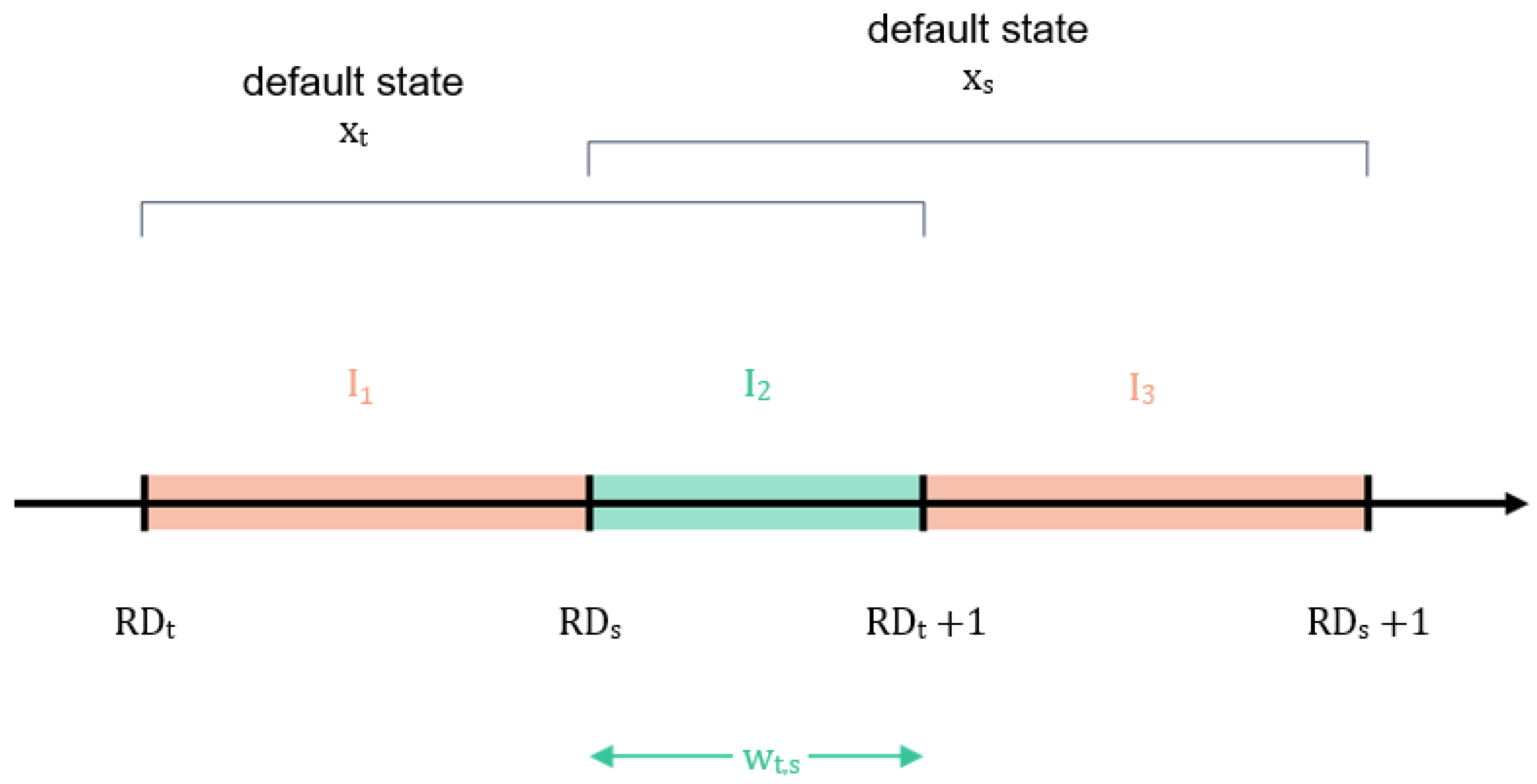
2.4. Covariance between Default States

Pursuant to Paragraph 80 EBA-GL (EBA GL 2017), when calculating the long-run default rate, institutions may choose between overlapping time windows of one year and non-overlapping time windows. According to Paragraph 78 EBA-GL, the reference dates used should include at least all quarterly reference dates. The overlap of the time windows of the one-year default rates leads to correlations between them, which affects the variance of the long-run default rate and thus the acceptance ranges of the test.

In order to be able to describe the distribution of the test statistic as precisely as possible, in Section 2.5 below, we thus focus on the analysis of the covariances between and the default rates, and start by considering the covariance between two default states of individual obligors for overlapping observation periods in this subsection. To that end, we consider two reference dates ${\mathrm{RD}}_t$ and ${\mathrm{RD}}_s$ with ${\mathrm{RD}}_t<{\mathrm{RD}}_s<{\mathrm{RD}}_t+1$ and an obligor who can be observed in the period $[{\mathrm{RD}}_t,{\mathrm{RD}}_s+1)$. The default state in the period $[{\mathrm{RD}}_t,{\mathrm{RD}}_t+1)$ is described by a random variable $x_t\in \left\{0,1\right\}$, the default state in the period $[{\mathrm{RD}}_s,{\mathrm{RD}}_s+1)$ by a random variable $x_s\in \left\{0,1\right\}$, cf. Figure 1. Throughout, default events correspond to realizations of the value 1 for default states. That is, a realization of $x_t$ or $x_s$ answers the question whether or not the obligor under consideration defaulted in time period $[{\mathrm{RD}}_t,{\mathrm{RD}}_t+1)$ or $[{\mathrm{RD}}_s,{\mathrm{RD}}_s+1)$, respectively.

In order to compute the covariance between the two default states $x_t$ and $x_s$, a detailed knowledge of the time of default is necessary, where, in the case of more than one default event, we focus on the time of the temporally first default. The time of first default is described by a random variable $T_1\in [{\mathrm{RD}}_t,\infty )$, which creates a link between default status and time of default, see, e.g., European Commission (2021). While $T_1$ describes the timing of the first default starting at time ${\mathrm{RD}}_t$, we model the timing of the first default after the default described by $T_1$ and after ${\mathrm{RD}}_s$ using a random variable $T_2^{*}\in [{\mathrm{RD}}_s,\infty )$, with $T_2^{*}>T_1$. We then define

$$T_2:=\left\{\begin{array}{cc}{T}_1,\hfill & \mathrm{if}{T}_1\ge {\mathrm{RD}}_s\mathrm{and}{T}_2^{*}>{\mathrm{RD}}_s+1,\hfill \\ T_2^{*},\hfill & \mathrm{otherwise}.\hfill \end{array}\right.$$

If besides $T_1$ more than one default is observed in the interval $[{\mathrm{RD}}_s,{\mathrm{RD}}_s+1)$, $T_2$ describes the time of the second default, otherwise $T_2$ is used to model the time of the first default starting from ${\mathrm{RD}}_s$. We now divide the considered time period into three disjoint intervals

$$I_1:=[{\mathrm{RD}}_t,{\mathrm{RD}}_s],I_2:=({\mathrm{RD}}_s,{\mathrm{RD}}_t+1],\mathrm{and}{I}_3:=({\mathrm{RD}}_t+1,{\mathrm{RD}}_s+1],$$

and look at the following disjoint events

$$E_1:=\{T_1\in I_1\},E_2:=\{T_1\in I_2\},\mathrm{and}{E}_3:=\{T_1\notin I_1\cup I_2\}.$$

Moreover, we define

$$E_4:=\{T_2\in I_2\},E_5:=\{T_2\in I_3\},\mathrm{and}{E}_6:=\{T_2\notin I_2\cup I_3\}.$$

In order to simplify notation, we set $p_t:=\mathbb{P}(x_t=1)$ and $p_s:=\mathbb{P}(x_s=1)$ and assume that

$$\mathbb{P}(x_t=1|E_5)=p_t\mathrm{and}\mathbb{P}(x_s=1|E_1)=p_s.$$

In a first step, we focus on the probability $\mathbb{P}\left(E_1\right)$. For this, we assume that the probability of default in a certain time interval depends on the length of this interval and on the general creditworthiness of the obligor, i.e., we assume that

$$\mathbb{P}(T_1\in I|x_t=1)=f_1\left(\right|I\left|\right)$$

for every interval $I\subseteq [{\mathrm{RD}}_t,{\mathrm{RD}}_t+1)$ and a non-negative and non-decreasing function $f_1$ with $f_1\left(0\right)=0$ and $f_1\left(1\right)=1$. This ensures that the probability of observing a default in a given time interval increases if the length of the interval increases and that the probabilities of default are identical for intervals of the same length. We deduce

$$\mathbb{P}\left(E_1\right|x_t=1)=1-\mathbb{P}\left(E_2\right|x_t=1)=1-f_1\left(w_{t,s}\right),$$

and therefore, using Bayes’ theorem,

$$1-f_1\left(w_{t,s}\right)=\mathbb{P}\left(E_1\right|x_t=1)=\mathbb{P}(x_t=1|E_1)·{\displaystyle \frac{\mathbb{P}\left(E_1\right)}{\mathbb{P}(x_t=1)}}={\displaystyle \frac{\mathbb{P}\left(E_1\right)}{p_t}}.$$

Rearranging terms, we find that

$$\mathbb{P}\left(E_1\right)=\left(1-f_1\left(w_{t,s}\right)\right)p_t$$

and, analogously,

$$\mathbb{P}\left(E_2\right)=f_1\left(w_{t,s}\right)p_t.$$

Hence,

$$\begin{array}{cc}\hfill \mathbb{E}(x_t·x_s)& =\mathbb{P}(x_t=1,x_s=1)=\mathbb{P}(x_t=1,x_s=1|E_1)·\mathbb{P}\left(E_1\right)\hfill \\ \hfill & +\mathbb{P}(x_t=1,x_s=1|E_2)·\mathbb{P}\left(E_2\right)+\mathbb{P}(x_t=1,x_s=1|E_3)·\mathbb{P}\left(E_3\right)\hfill \\ \hfill & =\mathbb{P}(x_s=1|E_1)·\mathbb{P}\left(E_1\right)+\mathbb{P}\left(E_2\right)=p_s\left(1-f_1\left(w_{t,s}\right)\right)p_t+f_1\left(w_{t,s}\right)p_t\hfill \\ \hfill & =p_t{p}_s+f_1\left(w_{t,s}\right)p_t(1-p_s).\hfill \end{array}$$

Analogously, one obtains

$$\mathbb{P}\left(E_4\right)=f_2\left(w_{t,s}\right)p_s\mathrm{and}\mathbb{P}\left(E_5\right)=\left(1-f_2\left(w_{t,s}\right)\right)p_s,$$

for a non-negative and non-decreasing function $f_2$ with $f_2\left(0\right)=0$ and $f_2\left(1\right)=1$, and we find that

$$\begin{array}{cc}\hfill \mathbb{E}(x_t·x_s)& =\mathbb{P}(x_t=1,x_s=1)=\mathbb{P}(x_t=1,x_s=1|E_4)·\mathbb{P}\left(E_4\right)\hfill \\ \hfill & +\mathbb{P}(x_t=1,x_s=1|E_5)·\mathbb{P}\left(E_5\right)+\mathbb{P}(x_t=1,x_s=1|E_6)·\mathbb{P}\left(E_6\right)\hfill \\ \hfill & =\mathbb{P}\left(E_4\right)+\mathbb{P}(x_t=1|E_5)·\mathbb{P}\left(E_5\right)=f_2\left(w_{t,s}\right)p_s+p_t\left(1-f_2\left(w_{t,s}\right)\right)p_s\hfill \\ \hfill & =p_t{p}_s+f_2\left(w_{t,s}\right)p_s(1-p_t).\hfill \end{array}$$

Equating the previous expectations results in

$$f_1\left(w_{t,s}\right)=f_2\left(w_{t,s}\right){\displaystyle \frac{p_s\left(1-p_t\right)}{p_t\left(1-p_s\right)}},$$

i.e., $f_1$ is a linear transform of $f_2$. To determine the covariance between $x_t$ and $x_s$, knowledge of at least one of the functions $f_1$ or $f_2$ is required. We assume that the distribution of the time of default within an observation year is uniform. We postulate this assumption for $x_s$, since it gives preference to the more recent information at ${\mathrm{RD}}_s$ over the information at ${\mathrm{RD}}_t$, which lies further in the past. We therefore set $f_2\left(w_{t,s}\right)=w_{t,s}$ and end up with

$$\mathrm{Cov}(x_t,x_s)=\mathbb{E}(x_t·x_s)-\mathbb{E}\left(x_t\right)·\mathbb{E}\left(x_s\right)=w_{t,s}{p}_s(1-p_t).$$

(5)

2.5. Covariance between Default Rates

Having previously examined the covariance between obligor default states, we extrapolate this result to the covariance of default rates. To do this, we consider a sample of debtors on reference dates ${\mathrm{RD}}_t$ and ${\mathrm{RD}}_s$ with ${\mathrm{RD}}_s<{\mathrm{RD}}_t+1$ and $t,s=1,\dots ,N$. During the transition from the first to the second reference date, debtors can be removed from monitoring due to defaults, terminated business relationships, or migrations to other rating systems, and new debtors can be added on the second reporting date due to new business or migrations to the rating system under consideration. In addition, there are debtors who can be observed on both reference dates. The number of these so-called persisting customers with respect to reference dates ${\mathrm{RD}}_t$ and ${\mathrm{RD}}_s$ is denoted by $\left|{\Lambda }_t\cap {\Lambda }_s\right|=:k_{t,s}\in \mathbb{N}$. The one-year default rates on the two reference dates are then given by $X_t={\displaystyle \frac{1}{n_t}}{\sum }_{j\in {\Lambda }_t}{x}_{t,j}$ with $x_{t,j}\sim B\left(1,p_{t,j}\right)$ and $X_s={\displaystyle \frac{1}{n_s}}{\sum }_{j\in {\Lambda }_s}{x}_{s,j}$ with $x_{s,j}\sim B\left(1,p_{s,j}\right)$. Hence,

$$\mathrm{Cov}\left(X_t,X_s\right)={\displaystyle \frac{1}{n_t{n}_s}}\sum _{i\in {\Lambda }_t}\sum _{j\in {\Lambda }_t}\mathrm{Cov}\left(x_{t,i},x_{s,j}\right).$$

Again, assuming that default states for pairs of different customers are independent, using Formula (5), we find that

$$\mathrm{Cov}\left(X_t,X_s\right)={\displaystyle \frac{1}{n_t{n}_s}}\sum _{j\in {\Lambda }_t\cap {\Lambda }_s}\mathrm{Cov}\left(x_{t,j},x_{s,j}\right)={\displaystyle \frac{w_{t,s}}{n_t{n}_s}}\sum _{j\in {\Lambda }_t\cap {\Lambda }_s}{p}_{s,j}\left(1-p_{t,j}\right),$$

(6)

where $w_{t,s}$ describes, as before, the size of the overlap between the observation periods starting from the reference dates ${\mathrm{RD}}_t$ and ${\mathrm{RD}}_s$.

2.6. Variance of the Long-Run Default Rate

Based on the considerations for estimating the covariance of default rates in overlapping periods, we now discuss the variance of the long-run default rate. For the random variable $X_t$ with $t=1,\dots ,N$, we define $\mathbb{E}\left(X_t\right)=:{\mu }_t$ and $\sigma \left(X_t\right)=:{\sigma }_t$. For the long-run default rate Z, which is approximately normally distributed with $Z\sim \mathcal{N}(\mu ,{\sigma }^2)$, we obtain

$$\mu ={\displaystyle \frac{1}{R\left(N\right)}}·\sum _{t=1}^N{\mu }_t={\displaystyle \frac{1}{R\left(N\right)}}·\sum _{t=1}^N{\displaystyle \frac{1}{n_t}}\sum _{j\in {\Lambda }_t}{p}_{t,j}$$

and

$$\begin{array}{cc}\hfill R{\left(N\right)}^2·{\sigma }^2& =\sum _{t=1}^N{\sigma }_t^2+2\sum _{t=1}^{N-1}\sum _{s=t+1}^N\mathrm{Cov}\left(X_t,X_s\right)\hfill \\ \hfill & =\sum _{t=1}^N{\sigma }_i^2+2\sum _{i=1}^{q-1}\sum _{t=1}^{N-i}\mathrm{Cov}\left(X_t,X_{t+i}\right),\hfill \end{array}$$

(7)

where the second term contains the covariances caused by overlapping time periods. Using Equation (6), we end up with

$$\begin{array}{cc}\hfill R{\left(N\right)}^2·{\sigma }^2=& \sum _{t=1}^N{\displaystyle \frac{1}{n_t^2}}\sum _{j\in {\Lambda }_t}{p}_{t,j}(1-p_{t,j})\hfill \\ \hfill & +\sum _{i=1}^{q-1}{\displaystyle \frac{2(q-i)}{q}}\sum _{t=1}^{N-i}{\displaystyle \frac{1}{n_t·n_{t+i}}}\sum _{j\in {\Lambda }_t\cap {\Lambda }_{t+i}}{p}_{t+i,j}(1-p_{t,j}).\hfill \end{array}$$

(8)

For the final calibration test, it will be crucial to estimate the variance of the long-run default rate by a term that solely depends on the expected value $\mu$, the number of debtors per reference date, and debtor-independent variables, see Section 3.2.

3. Hypothesis Test for Long-Term Calibration

The aim of this section is to formulate a statistical test for comparing the realized long-run default rate with the estimated long-run default rate.

3.1. Statistical Test per Rating Grade

We start with the simplest case and consider a portfolio consisting of only one rating grade with an associated probability of default, which we call ${\mathrm{PD}}_{\mathrm{grade}}$. That is, all considered obligors have the same unknown probability of default, which was estimated by ${\mathrm{PD}}_{\mathrm{grade}}$. We recall that the measured long-run default rate, denoted by $\mathrm{LRDR}$, is the realization of a random variable Z for which approximately $Z\sim \mathcal{N}(\mu ,{\sigma }^2)$ holds. We consider the hypothesis test, described in Section 2.2, with

$$\begin{array}{cc}\hfill & \mathrm{null}\mathrm{hypothesis}{H}_0:\mu ={\mathrm{PD}}_{\mathrm{grade}}\mathrm{and}\hfill \\ \hfill & \mathrm{alternative}\mathrm{hypothesis}{H}_1:\mu \ne {\mathrm{PD}}_{\mathrm{grade}}.\hfill \end{array}$$

From Equation (8), we obtain

$$\begin{array}{cc}\hfill R{\left(N\right)}^2·{\sigma }^2& =\sum _{t=1}^N{{\sigma }_t}^2+\sum _{i=1}^{q-1}{\displaystyle \frac{2(q-i)}{q}}\sum _{t=1}^{N-i}{\displaystyle \frac{1}{n_t·n_{t+i}}}\sum _{j\in {\Lambda }_t\cap {\Lambda }_{t+i}}\mu \left(1-\mu \right)\hfill \\ \hfill & =\sum _{t=1}^N{{\sigma }_t}^2+\mu \left(1-\mu \right)\sum _{i=1}^{q-1}{\displaystyle \frac{2(q-i)}{q}}\sum _{t=1}^{N-i}{\displaystyle \frac{k_{t,t+i}}{n_t·n_{t+i}}}\hfill \\ \hfill & =\sum _{t=1}^N{{\sigma }_t}^2+\mu \left(1-\mu \right)\sum _{i=1}^{q-1}{\lambda }_i,\hfill \end{array}$$

where

$${\lambda }_i:={\displaystyle \frac{2(q-i)}{q}}\sum _{t=1}^{N-i}{\displaystyle \frac{k_{t,t+i}}{n_t·n_{t+i}}}.$$

Moreover,

$$\sum _{t=1}^N{{\sigma }_t}^2=\sum _{t\in R_N}{\displaystyle \frac{1}{n_t}}·\mu \left(1-\mu \right)=\mu \left(1-\mu \right)\sum _{t\in R_N}{\displaystyle \frac{1}{n_t}},$$

which implies that

$${\sigma }^2={\displaystyle \frac{\mu \left(1-\mu \right)}{R{\left(N\right)}^2}}\left(\sum _{t\in R_N}{\displaystyle \frac{1}{n_t}}+\sum _{i=1}^{q-1}{\lambda }_i\right).$$

Therefore, assuming the validity of the null hypothesis, $\sigma$ is known. In order to define the limits of the acceptance range for a significance level $\alpha \in \left(0,1\right)$, we choose $k,K\in [0,1]$ in such a way that

$$\mathbb{E}\left(\phi \left(Z\right)\right){|}_{H_0}\le \alpha ,$$

where $\phi$ is given by (3). To that end, let

$$k={\mathrm{PD}}_{\mathrm{grade}}+{\Phi }^{-1}\left({\displaystyle \frac{1}{2}}\alpha \right)·\sqrt{{\displaystyle \frac{{\mathrm{PD}}_{\mathrm{grade}}\left(1-{\mathrm{PD}}_{\mathrm{grade}}\right)}{R{\left(N\right)}^2}}\left(\sum _{t\in R_N}{\displaystyle \frac{1}{n_t}}+\sum _{i=1}^{q-1}{\lambda }_i\right)}$$

and

$$K={\mathrm{PD}}_{\mathrm{grade}}+{\Phi }^{-1}\left(1-{\displaystyle \frac{1}{2}}\alpha \right)·\sqrt{{\displaystyle \frac{{\mathrm{PD}}_{\mathrm{grade}}\left(1-{\mathrm{PD}}_{\mathrm{grade}}\right)}{R{\left(N\right)}^2}}\left(\sum _{t\in R_N}{\displaystyle \frac{1}{n_t}}+\sum _{i=1}^{q-1}{\lambda }_i\right)}.$$

Then, the calibration test passes if

$$\mathrm{LRDR}\in \left[k,K\right].$$

To see the influence of persisting customers on the acceptance range and the density function of the long-run default rate, we refer to Section 4.1 and Section 4.2.

3.2. Statistical Test on Portfolio Level

We now consider a portfolio of heterogeneous obligors, i.e., each obligor has its own individual probability of default. For this purpose, we denote the estimated PD of customer j on reference date ${\mathrm{RD}}_t$ by ${\widehat{p}}_{t,j}$, the mean PD based on the rating model examined on the reference date ${\mathrm{RD}}_t$ by ${\widehat{\mathrm{PD}}}_t$ for $t=1,\dots ,N$, and the long-run central tendency by

$$\mathrm{LRCT}={\displaystyle \frac{1}{N}}·\sum _{t=1}^N{\widehat{\mathrm{PD}}}_t={\displaystyle \frac{1}{N}}·\sum _{t=1}^N{\displaystyle \frac{1}{n_t}}\sum _{j\in {\Lambda }_t}{\widehat{p}}_{t,j}.$$

While on the level of rating grades, it is not an exception that the number of customers at a reference date ${\mathrm{RD}}_t$ might be zero, i.e., $n_t=0$, on a portfolio level, though this rarely happens in practice. In this section, we therefore restrict our attention to the case where $n_t>0$ for all $t=1,\dots ,N$ and therefore $R\left(N\right)=N$.

We consider the hypothesis test from Section 2.2 with

$$\begin{array}{cc}\hfill & \mathrm{null}\mathrm{hypothesis}{H}_0:\mu =\mathrm{LRCT}\mathrm{and}\hfill \\ \hfill & \mathrm{alternative}\mathrm{hypothesis}{H}_1:\mu \ne \mathrm{LRCT}.\hfill \end{array}$$

As in the case of individual rating grades, the test statistic depends on $\mu$ and $\sigma$ but, in this case, Equation (8) can no longer be reduced to a term depending only on $\mu$. More precisely, if the correctness of the null hypothesis is assumed, the distribution parameters are only partially determined. If, however, we replace $\sigma$ by an expression ${\sigma }_{min}\left(\mu \right)$ with $\sigma \ge {\sigma }_{min}\left(\mu \right)$, the null hypothesis implies a concrete distribution for the underlying test statistic. This results in a narrower confidence interval and therefore a greater likelihood of committing a type I error. At the same time, the probability of a type II error is reduced, comparable to lowering the significance level.

The key challenge is to derive an analytic expression for ${\sigma }_{min}$ that depends only on PD-independent model parameters, such as N, M, $n_t$, etc., and satisfies ${\sigma }_{min}\left(\mu \right)\le \sigma$ under the null hypothesis for all possible combinations of $p_{t,j}\in [{\mathrm{PD}}_{min},{\mathrm{PD}}_{max}]$. Since we aim to minimize the distance between ${\sigma }_{min}\left(\mu \right)$ and $\sigma$, it is sensible to define ${\sigma }_{min}$ via the solution to a minimization problem with cost functional given by the right-hand side of (8) under the side condition

$$\mu ={\displaystyle \frac{1}{N}}·\sum _{t=1}^N{\displaystyle \frac{1}{n_t}}\sum _{j\in {\Lambda }_t}{p}_{t,j}\mathrm{and}{p}_{t,j}\in [{\mathrm{PD}}_{min},{\mathrm{PD}}_{max}].$$

(9)

Observe that the right-hand side of (8) is, in general, neither convex nor concave with respect to the $p_{t,j}$. This, together with the high dimensionality of the problem, means the numerical or analytical computation of solutions is rather involved. In order to circumvent this issue, we therefore replace the right-hand side of (8) by a suitable linear cost functional, which turns the minimization into a linear program that can be solved analytically, up to a sort algorithm, and therefore also numerically with great efficiency.

First, note that mixed terms, i.e., products of PDs of the same customer at different reference dates, always appear in the sums

$$\sum _{j\in {\Lambda }_t\cap {\Lambda }_{t+i}}{p}_{t+i,j}\left(1-p_{t,j}\right)$$

caused by the covariances. Hence, in Formula (8), we want to substitute the subtrahend (blue) by an affine linear function with respect to the multiplier (orange) in a conservative way. On a portfolio level, it is appropriate to assume that an obligor’s PD remains constant on average over a one-year time horizon, i.e., we assume

$$\sum _{j\in {\Lambda }_t\cap {\Lambda }_{t+i}}{p}_{t+i,j}\left(1-p_{t,j}\right)\approx \sum _{j\in {\Lambda }_t\cap {\Lambda }_{t+l}}{p}_{t+i,j}\left(1-p_{t+i,j}\right).$$

(10)

For most portfolios, this is not only a plausible but also a fairly conservative assumption regarding the portfolio variance since, for a given vector $(x_1,\dots ,x_n)$ with $0<x_i<1$ for $i=1,\dots ,n$, the sum

$$\sum _{i=1}^n{x}_i(1-y_i)$$

is minimized for $x_i=y_i$, under the assumption that, for each $i=1,\dots ,n$, there exists some $j=1,\dots ,n$ with $x_i=y_j$. Certainly, even more conservative assumptions can be made at this point with ${\mathrm{PD}}_{max}$ being the most conservative subtrahend possible. The impact of such a choice is discussed in Section 4.6, where we indicate that the acceptance ranges hardly change when using ${\mathrm{PD}}_{max}$ instead of $p_{t+i,j}$. We point out that the subsequent discussion applies also to this choice without limitations.

From Equation (8), we obtain

$$\begin{array}{cc}\hfill N^2·{\sigma }^2& =\sum _{t=1}^N{\displaystyle \frac{1}{n_t^2}}\sum _{j\in {\Lambda }_t}{p}_{t,j}(1-p_{t,j})\hfill \\ \hfill & +\sum _{i=1}^{q-1}{\displaystyle \frac{2(q-i)}{q}}\sum _{t=1}^{N-i}{\displaystyle \frac{1}{n_t·n_{t+i}}}\sum _{j\in {\Lambda }_t\cap {\Lambda }_{t+i}}{p}_{t+i,j}(1-p_{t+i,j})\hfill \\ \hfill & =\sum _{t=1}^N{\displaystyle \frac{1}{n_t^2}}\sum _{j\in {\Lambda }_t}{g}_0\left(p_{t,j}\right)+2\sum _{i=1}^{q-1}\sum _{t=1}^{N-i}{\displaystyle \frac{1}{n_t·n_{t+i}}}\sum _{j\in {\Lambda }_t\cap {\Lambda }_{t+i}}{g}_i\left(p_{t+i,j}\right)\hfill \end{array}$$

with

$$g_i\left(x\right):={\displaystyle \frac{q-i}{q}}·x\left(1-x\right)\mathrm{for}x\in (0,1)\mathrm{and}i=0,\dots ,q-1.$$

Now, we replace each of the functions $g_i$ by an affine linear function $f_i$ such that the functions $g_i$ and $f_i$ coincide on ${\mathrm{PD}}_{max}$ and ${\mathrm{PD}}_{min}$. Since $g_i$ is concave and $f_i$ is affine linear, this implies that $g_i\left(x\right)\ge f_i\left(x\right)$ for all $x\in [{\mathrm{PD}}_{min},{\mathrm{PD}}_{max}]$. To be precise, the functions $f_i$ are given by

$$f_i\left(x\right):={\alpha }_i·x+c_i\mathrm{for}\mathrm{all}x\in (0,1)$$

with

$$\begin{array}{c}\hfill {\alpha }_i:={\displaystyle \frac{q-i}{q}}(1-{\mathrm{PD}}_{max}-{\mathrm{PD}}_{min})\mathrm{and}{c}_i={\displaystyle \frac{q-i}{q}}{\mathrm{PD}}_{min}{\mathrm{PD}}_{max}\end{array}$$

for all $i=0,\dots ,q-1$. We therefore end up with the estimate

$$\begin{array}{cc}\hfill N^2·{\sigma }^2& =\sum _{t=1}^N{\displaystyle \frac{1}{n_t^2}}\sum _{j\in {\Lambda }_t}{g}_0\left(p_{t,j}\right)+2\sum _{i=1}^{q-1}\sum _{t=1}^{N-i}{\displaystyle \frac{1}{n_t·n_{t+i}}}\sum _{j\in {\Lambda }_t\cap {\Lambda }_{t+i}}{g}_i\left(p_{t+i,j}\right)\hfill \\ \hfill & \ge \sum _{t=1}^N{\displaystyle \frac{1}{n_t^2}}\sum _{j\in {\Lambda }_t}{f}_0\left(p_{t,j}\right)+2\sum _{i=1}^{q-1}\sum _{t=1}^{N-i}{\displaystyle \frac{1}{n_t·n_{t+i}}}\sum _{j\in {\Lambda }_t\cap {\Lambda }_{t+i}}{f}_i\left(p_{t+i,j}\right)\hfill \\ \hfill & =\sum _{t=1}^N{\displaystyle \frac{1}{n_t^2}}\sum _{j\in {\Lambda }_t}({\alpha }_0·p_{t,j}+c_0)+2\sum _{i=1}^{q-1}\sum _{t=1}^{N-i}{\displaystyle \frac{1}{n_t·n_{t+i}}}\sum _{j\in {\Lambda }_t\cap {\Lambda }_{t+i}}({\alpha }_i·p_{t+i,j}+c_i)\hfill \\ \hfill & =\sum _{t=1}^N\sum _{j\in {\Lambda }_t}{\alpha }_{t,j}{p}_{t,j}+C,\hfill \end{array}$$

(11)

where in the last step, we have isolated all terms that do not depend on $p_{t,j}$ in the constant C by using $k_{t,t+i}=\left|{\Lambda }_t\cap {\Lambda }_{t+i}\right|$, i.e.,

$$\begin{array}{c}\hfill C=c_0·\sum _{t=1}^N{\displaystyle \frac{1}{n_t}}+2·\sum _{i=1}^{q-1}{c}_i·\sum _{t=1}^{N-i}{\displaystyle \frac{k_{t,t+i}}{n_t·n_{t+i}}}\end{array}$$

and

$$\begin{array}{c}\hfill {\alpha }_{t,j}={\displaystyle \frac{1}{n_t^2}}{\alpha }_0{\mathbb{1}}_{{\Lambda }_t}\left(j\right)+{\displaystyle \frac{2}{n_t}}·\sum _{i=1}^{q-1}{\displaystyle \frac{{\alpha }_i}{n_{t-i}}}{\mathbb{1}}_{{\Lambda }_{t-i}\cap {\Lambda }_t}\left(j\right)\end{array}$$

with ${\Lambda }_{t-i}:=\varnothing$ if $t-i<1$ for $t=1,\dots ,N$ and $j=1,\dots ,M$. We have therefore reduced the original problem to

$$\mathrm{minimize}\sum _{t=1}^N\sum _{j\in {\Lambda }_t}{\alpha }_{t,j}{p}_{t,j}\mathrm{under}\mathrm{the}\mathrm{side}\mathrm{condition}(9).$$

(12)

As shown in Appendix A, the solution $p\left(\mu \right)$ to the minimization problem (12) can be easily computed analytically and numerically. We denote the minimal value by $m\left(\mu \right)$, and define ${\sigma }_{min}^2\left(\mu \right)={\displaystyle \frac{m\left(\mu \right)+C}{N^2}}$.

For the modified random variable $Z^{*}\sim \mathcal{N}\left(\mu ,{\sigma }_{min}^2\left(\mu \right)\right)$, we are now able to define the limits $k,K\in [0,1]$ of the acceptance range for a significance level $\alpha \in \left(0,1\right)$ in such a way that $\mathbb{E}\left(\phi \left(Z^{*}\right)\right){|}_{H_0}\le \alpha .$ For this, we define

$$k:=\mathrm{LRCT}+{\Phi }^{-1}\left({\displaystyle \frac{1}{2}}\alpha \right)·{\sigma }_{min}\left(\mathrm{LRCT}\right)$$

and

$$K:=\mathrm{LRCT}+{\Phi }^{-1}\left(1-{\displaystyle \frac{1}{2}}\alpha \right)·{\sigma }_{min}\left(\mathrm{LRCT}\right).$$

The calibration test passes if

$$\mathrm{LRDR}\in \left[k,K\right].$$

4. Discussion and Further Considerations

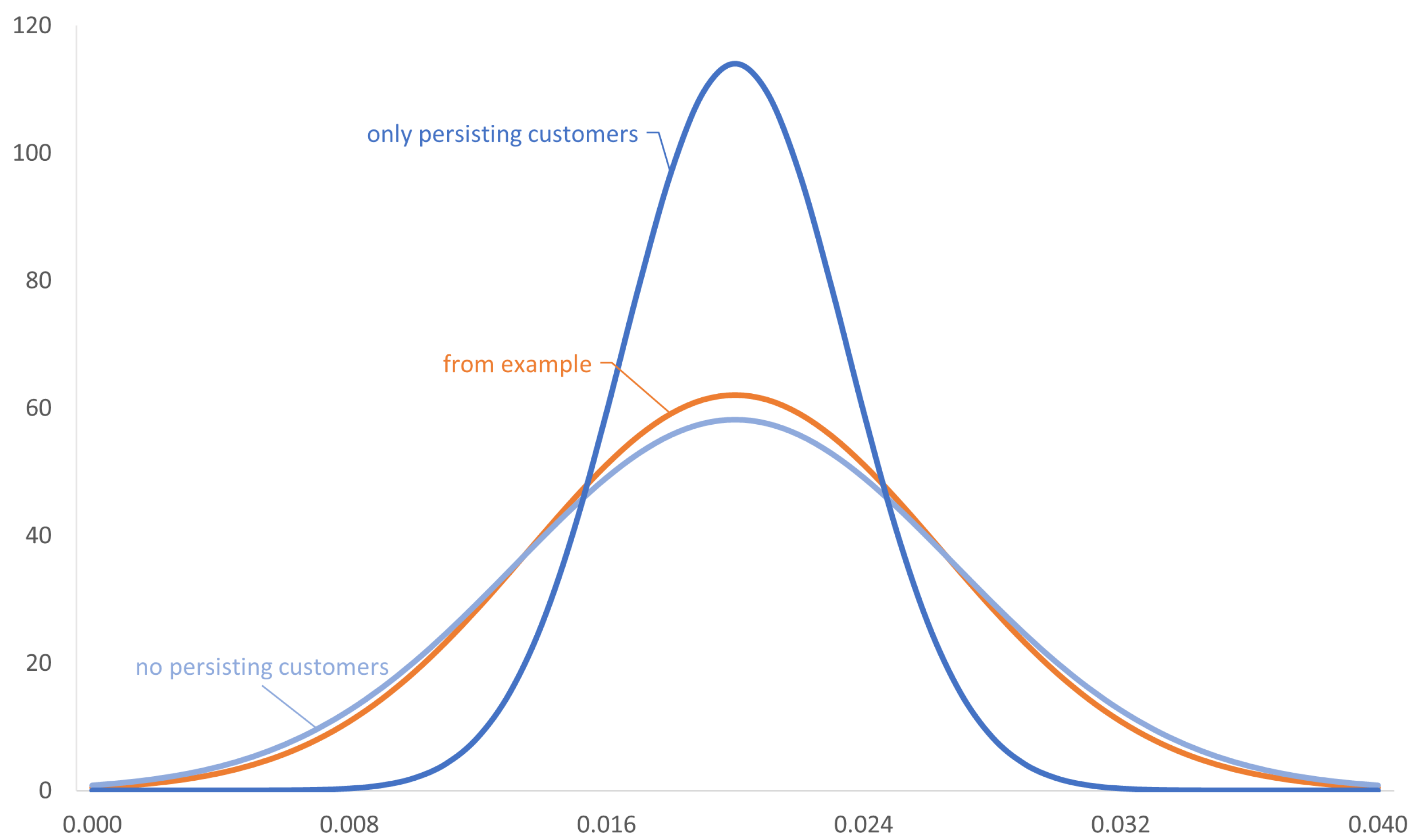
4.1. Effect of Persisting Customers on the Variance of Z

In this section, we aim to highlight the effects caused by persisting customers on the distribution of Z. We calculate the density function of the long-run default rate using a sample portfolio in a rating grade with $\mathrm{PD}=0.02$ and set $q=4$. The number of reference dates is $N=R\left(N\right)=32$, i.e., we consider a portfolio with a relatively short history of eight years. The number of customers is set to be constant over time with $n=50$. We furthermore assume that the ratio of persisting customers per time interval is constant over time. We have $k_{t,t+1}=45$ for all $t\le 31$, $k_{t,t+2}=40$ for all $t\le 30$, and $k_{t,t+3}=35$ for all $t\le 29$. Only about $70\%$ of the persisting customers are still in the considered rating grade after three- quarters, which represents a relatively high fluctuation.

These specifications determine the density function of the long-run default rate (orange). In comparison, one can see the density functions of the long-run default rate with a maximum and minimum number of persisting customers in gray and blue, respectively. We have

$${\sigma }_{\mathrm{orange}}^2\approx 4.13·{10}^{-5},{\sigma }_{\mathrm{blue}}^2\approx 1.23·{10}^{-5},\mathrm{and}{\sigma }_{\mathrm{gray}}^2\approx 4.71·{10}^{-5}.$$

Figure 2 shows that that correlation effects caused by overlapping time windows should not be neglected since, otherwise, the acceptance range would be way too tight, see also Section 4.2 below.

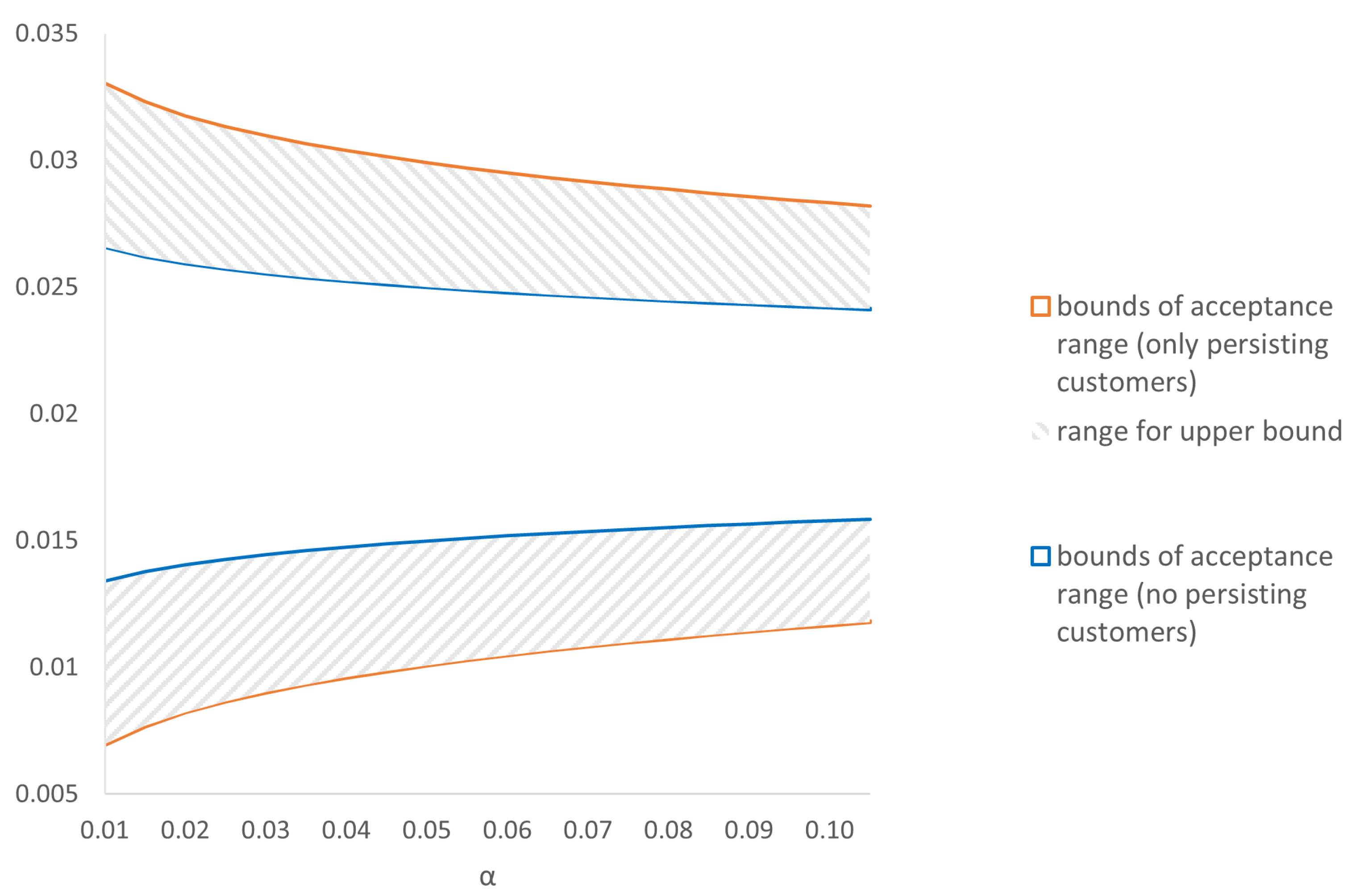
4.2. Effect of Persisting Customers on Acceptance Range

We examine the influence of the number of persisting customers on the width of the acceptance range. Again, we choose $q=4$ and, for the sake of simplicity, we consider the case at the level of the individual grades choosing ${\mathrm{PD}}_{\mathrm{grade}}=0.02$. The proportion of persisting customers is usually lower at the level of individual grades than in the overall portfolio, since a rating migration automatically means that the customer in question is no longer in the sample for the individual grade but is still in the overall portfolio.

The number of reference dates is $N=R\left(N\right)=60$ and the number of customers is constant, i.e., $n_t:=n=50$ for $t=1,\dots ,50$. The extreme cases regarding persisting customers now represent the two scenarios in which, on the one hand, all customers remain the same over the entire history and, on the other hand, none of the customers in a specific quarter occurs in the previous quarter or in the following quarter.

The first case implies $k_{t,t+1}=n$ for $t\le N-1$, $k_{t,t+2}=n$ for $t\le N-2$ and $k_{t,t+3}=n$ for $t\le N-3$. Thus, for two one-year default rates $X_t$ and $X_s$ where $1\le t<s\le 50$, we have

$$\mathrm{Cov}\left(X_t,X_s\right)={\displaystyle \frac{1}{n}}·w_{t,s}\left(1-{\mathrm{PD}}_{\mathrm{grade}}\right)·{\mathrm{PD}}_{\mathrm{grade}}.$$

For the second case, we have $k_{t,t+1}=0$ for $t\le N-1$, $k_{t,t+2}=0$ for $t\le N-2$ and $k_{t,t+3}=0$ for $t\le N-3$, implying

$$\mathrm{Cov}\left(X_t,X_s\right)=0$$

for two one-year default rates $X_t$ and $X_s$. Since the covariance between default rates is always 0, in this case, the distribution of the long-run default rate is the same as if correlation effects due to overlapping time windows were ignored completely. Note that such a scenario is extremely unlikely, especially for a large number of ratings, and is therefore purely hypothetical since customers would constantly switch rating grades, which would imply a high level of instability in the rating system.

In Figure 3, we can see that the width of the acceptance range to a given level $\alpha$ for a portfolio only consisting of persisting customers is almost doubled compared to a portfolio with no persisting customers with respect to a three-month time horizon. A similar picture emerges when comparing the density functions of the long-run default rates, cf. Figure 4.

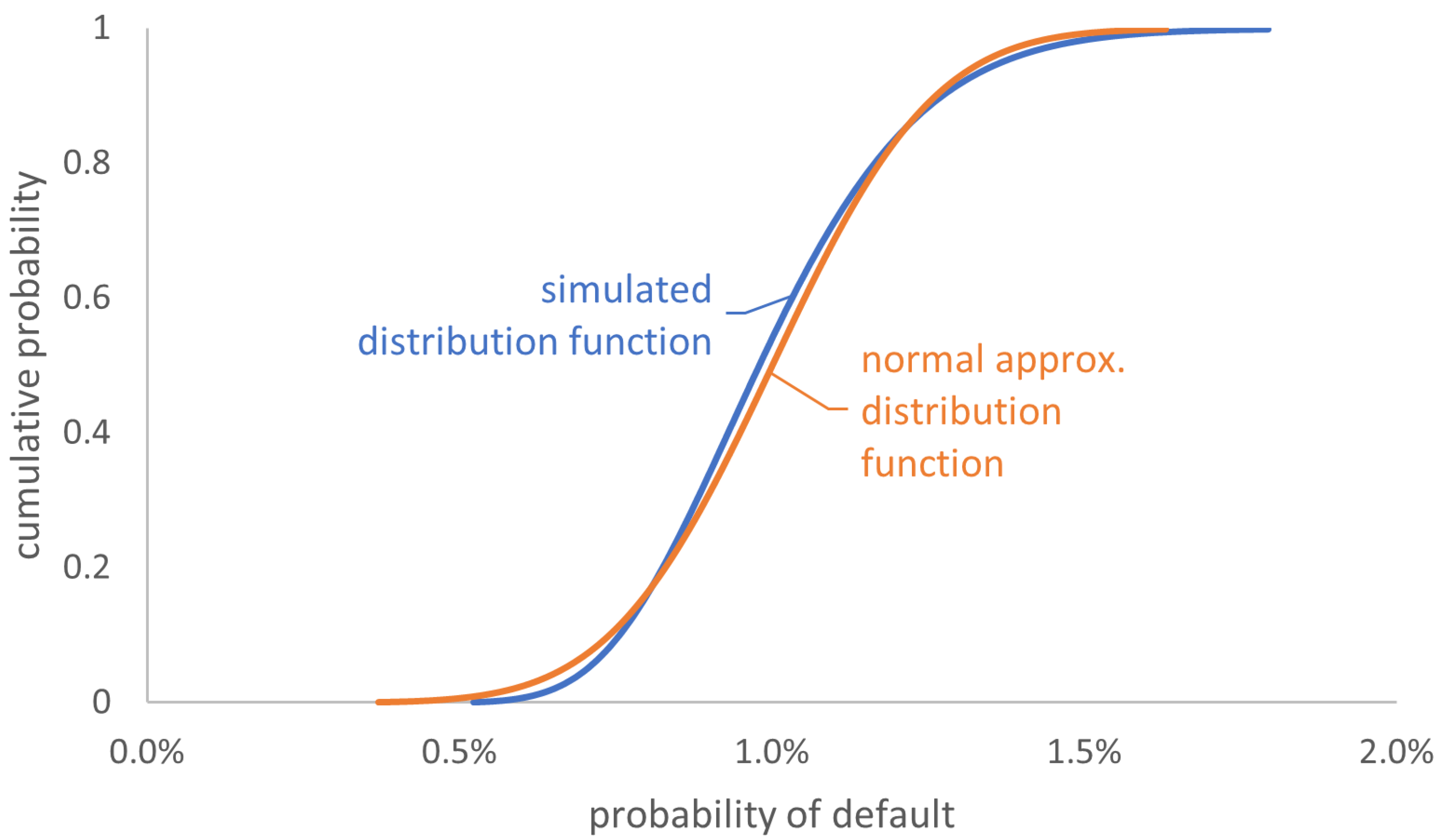
4.3. Some Thoughts on the Rate of Convergence

In view of Section 2.3, we briefly discuss the rate of convergence and mention a few particularities that need to be taken into account concerning the asymptotic behavior of the long-run default rate Z. When using the classical central limit theorem, it is common to specify a minimum number of random variables ensuring a reasonable approximation of the normal distribution. In our case, additional factors need to be taken into account since, for example, a large number of customers, i.e., a large number M in

$$Z={\displaystyle \frac{1}{N}}\sum _{t=1}^N{\displaystyle \frac{1}{n_t}}\sum _{j=1}^M{y}_{t,j}=\sum _{j=1}^M{Y}_j,$$

does not directly lead to a good approximation. This stems from the calculation logic of the long-run default rate. For a simple illustration, we assume that we are in the setting, where all customers have the same PD with $\mathrm{PD}=0.01$. For $N=1$ and $M=1000$ or, analogously, $N=1000$ and $n_t=1$ for $t=1,\dots ,1000$, the normal approximation is considerably better than for $N=2$ with $n_1=1$ and $n_2=999$ since, in the first case, $\mathbb{P}(Z\ge 0,5)\approx 0$ while, in the second case, $\mathbb{P}(Z\ge 0,5)>0,01.$ Thus, the rate of convergence depends on the number of customers, the number of reference dates, and the number of customers per reference date. While the previously described scenarios are uncommon at portfolio level, at the level of individual rating grades, constellations can arise in which, on certain reference dates, there is only one customer in the corresponding rating grade.

In the sequel, we elaborate more on this particularity and aim to provide a rule of thumb, i.e., conditions for N, $n_{max}$, and $n_{min}$ that imply a satisfactory normal approximation. To that end, we consider a synthetic portfolio. For the sake of simplicity, we assume that $q=1$ and simulate a convolution of weighted binomial distributions. We study the difference between the distribution functions of the long-run default rate on the level of a rating grade with $\mathrm{PD}=0.01$ when using a simulation on the one hand and using the normal approximation on the other hand in different scenarios. We assume the number of reference dates is $N=56$. The number of customers $n_t$ per reference date ${\mathrm{RD}}_t$ and thus the number of all customers M in the portfolio varies between the considered scenarios.

In Figure 5, there are eight reference dates where only one to five customers are in the portfolio. On the other reference dates, we assume the number of customers to be constant with $n_t=100$. We observe large differences in the two distribution functions, especially in the tails, which are particularly relevant for the test. If we now increase the number of customers on the critical reference dates (those with $n_t\le 5$) to 10, we observe, in Figure 6, that the distribution functions are almost the same. Hence, the poor convergence in Figure 5 is caused by the few reference dates with very few customers. Furthermore, we see that, in this special case, ${\displaystyle \frac{n_{min}}{n_{max}}}\ge {\displaystyle \frac{1}{10}}$ seems to be an appropriate bound in order to obtain a satisfactory approximation.

For a second comparison, we now reduce the number of customers significantly to $1\le n_t\le 10$. Again, the number of customers equals one only on the first eight reference dates. In Figure 7, we still see major differences in the distribution functions. Doubling the number of customers leads to Figure 8, where we already obtain useful results.

On the other hand, if the number of customers is very low, e.g., $n_t=2$ for half of all reference dates, we still obtain a good approximation, cf. Figure 9.

From our examples and statements from the literature, we conclude that $N\ge 30$, $n_{min}\ge 2$, and ${\displaystyle \frac{n_{min}}{n_{max}}}\ge {\displaystyle \frac{1}{10}}$ seem to be useful conditions to guarantee a satisfying normal approximation.

4.4. An Alternative Way to Bound the Variance

In Appendix B, we propose a different way to estimate the variance in an even more conservative way. If one accepts the associated stricter test as a conservative check of the calibration, one can use

$${\sigma }_{\mathrm{alt}}^2\left(\mu \right):={\displaystyle \frac{1}{N}}\left(C+K_1\right)\mu -{\displaystyle \frac{K_2}{N^2}}$$

as the variance of the test statistic with parameters $K_1$ and $K_2$ depending only on the underlying portfolio, see Appendix B for the details.

In this case, we do not have to solve an optimization problem, and can determine the variance directly using the portfolio-specific parameters. However, we additionally need conservative estimates for two parameters that are not directly determined by the null hypothesis. Again, we refer to Appendix B for the details. We briefly discuss the consequences of this alternative method at this point.

The determination of ${\sigma }_{\mathrm{alt}}^2\left(\mu \right)$ is based on a successive estimation of the variance of the test statistic against the maximum conservative value in each single step. This procedure can therefore be understood as a maximally conservative solution to the test problem. In the case of a portfolio with approximately constant size, approximately constant distribution of default probabilities over time, and no other special features, the conservatism can often be tolerated. In case of build-up or run-down portfolios or portfolios with a focus on high investment grade obligors, the risk of a type I error may become disproportionately large and the test may therefore not be suitable. This can be easily illustrated by the following two points. The estimation of quadratic terms on the left-hand side of (A6) is performed using ${\mathrm{PD}}_{max}$ regardless of how many obligors belong to the associated rating grade. For portfolios with mainly obligors with good ratings, this estimate is certainly too conservative. Moreover, the parameters $K_1$ and $K_2$ depend on

$$min\left\{{\displaystyle \frac{1}{n_t}}|t=1,\dots ,N\mathrm{and}{n}_t>0\right\}\mathrm{and}min\left\{k_{t,t+i}|t=1,\dots ,N-i\right\},$$

i.e., for portfolios where the number of customers or the number of persisting customers changes strongly over time, a lot of information is lost with this method. Thus, the estimate on the variance of the test statistic in Section 3.2 is much less conservative and suitable for significantly more portfolios.

4.5. Additional Conditions on the Rating Distribution

In this section, we give an outlook and offer suggestions as to which requirements can be placed on rating distributions. The implementation of some suggestions is briefly outlined. The rating distribution of $p\left(\mu \right)$ obtained by minimizing (12) tends to be U-shaped, cf. Figure 10, with all but at most one rating in the best or the worst rating grade. A U-shaped rating distribution, i.e., a distribution almost exclusively between the two extreme grades, is highly unusual, both in the case of a large number of ratings and in a portfolio that hardly has any customers in the lower rating grade.

Moreover, high values of ${\mathrm{PD}}_{max}$ lead to a narrowing of the acceptance range. Depending on the portfolio, this reduction can be disproportionately strong if, for example, the bad rating grades in low-default portfolios are heavily underrepresented. Hence, the question may be raised why the rating distribution, estimated by the rating model, is not used directly. As already mentioned, this would, however, require assumptions that go far beyond the null hypothesis, and specifying the rating distribution in that way would automatically determine the null hypothesis. However, it may be sensible to place additional yet conservative conditions on the rating distribution in (9).

For example, one could demand that ratings exhibit a conservative distribution, given by a function ${\phi }_1:\{{\mathrm{PD}}_{m-n+1},\dots ,{\mathrm{PD}}_m\}\to [0,1]$ across the n worst rating grades with

$$\mathbb{P}\left(p_{t,j}={\mathrm{PD}}_k|p_{t,j}\ge {\mathrm{PD}}_{m-n+1}\right)={\phi }_1\left({\mathrm{PD}}_k\right)\mathrm{for}k\ge m-n+1.$$

For most portfolios, a conservative choice of ${\phi }_1$ would be ${\phi }_1\left({\mathrm{PD}}_k\right)={\displaystyle \frac{1}{n}}$, cf. Figure 11.

Another approach would be to trust the distribution estimated by the rating model to some extent, and require that there is at least a fixed fraction $\delta \in [0,1]$ of the number of ratings per grade given by this distribution with density ${\phi }_2:\{{\mathrm{PD}}_1,\dots ,{\mathrm{PD}}_m\}\to [0,1]$. Then, in addition to (9), one might demand

$$n\left({\mathrm{PD}}_k\right)\ge n_{min}\left({\mathrm{PD}}_k\right):=⌊\sum _{t=1}^N{n}_t·{\phi }_2\left({\mathrm{PD}}_k\right)·\delta ⌋,$$

where $n\left({\mathrm{PD}}_k\right)$ is the number of the ratings in rating grade k, cf. Figure 12.

We conclude this section with a modified version of a previously described approach using a uniform distribution among the n worst rating grades. As before, we consider the n worst rating grades $\left\{{\mathrm{PD}}_{m-n+1},\dots ,{\mathrm{PD}}_m\right\}$ with ${\mathrm{PD}}_{m-n+1}>\mu$. Our aim is to formulate the requirement of a uniform distribution in such a way that we can again use the method for minimizing the variance already presented. To that end, we define

$$\overline{\mathrm{PD}}:={\displaystyle \frac{1}{n}}\sum _{i=m-n+1}^m{\mathrm{PD}}_i.$$

We follow the idea from Section 3.2, and proceed exactly as in Appendix A with $\overline{\mathrm{PD}}$ instead of ${\mathrm{PD}}_{max}$. The effect on the variance or, almost equivalently, the acceptance range is illustrated in Figure 13. On the one hand, this approach avoids unnecessary high conservatism. On the other hand, it is still sufficiently conservative and simple to implement.

4.6. Impact of Simplification on the Acceptance Range

In this section, we discuss how different choices of affine linear functions for the simplification of the variance effect the acceptance range. We focus on the impact when choosing either the constant function $g={\mathrm{PD}}_{max}$ or identity function as in (10).

We start by computing the reduction in the acceptance range due to choosing the affine linear function as the constant ${\mathrm{PD}}_{max}$ using a synthetic portfolio. We choose the number of customers per reference date to be constant with $n=1000$, let the number of reference dates be $N=60$, and $q=4$. We define ${\mathrm{PD}}_{max}=0.2$, ${\mathrm{PD}}_{min}=0.0003$, and set $\mu =0.01$. We recall that the components of the minimal solution $p\left(\mu \right)$ of (12) consist only of ${\mathrm{PD}}_{max}$, ${\mathrm{PD}}_{min}$, and ${\mu }_{k_0+1}$, where the latter is uniquely determined by the minimization problem.

We now choose $g={\mathrm{PD}}_{max}$, i.e., the most conservative function possible. Proceeding exactly as in Section 3.2 and in Appendix A, we simply obtain different values for ${\alpha }_i$ and $c_i$ with $i=0,\dots ,q-1$, namely,

$$\begin{array}{ccc}\hfill {\alpha }_i& =& {\displaystyle \frac{q-i}{q}}(1-{\mathrm{PD}}_{max}),\hfill \\ \hfill c_i& =& 0.\hfill \end{array}$$

Estimating the variance as in Section 3.2, once with $g={\mathrm{PD}}_{max}$ and once with $g=\mathrm{id}$, we obtain

$${\displaystyle \frac{\left|K\left({\mathrm{PD}}_{max}\right)-k\left({\mathrm{PD}}_{max}\right)\right|}{\left|K\left(\mathrm{id}\right)-k\left(\mathrm{id}\right)\right|}}\approx 0.994,$$

(13)

where $K\left({\mathrm{PD}}_{max}\right)$ and $k\left({\mathrm{PD}}_{max}\right)$ and $K\left(\mathrm{id}\right)$ and $k\left(\mathrm{id}\right)$ denote the upper and lower bound of the acceptance range for $g={\mathrm{PD}}_{max}$ and $g=\mathrm{id}$, respectively. In this particular setting, we see that the choice of g does not have a substantial influence on the size of the acceptance range.

The difference in the size of the acceptance range is largely influenced by the contributions of the obligors with $\mathrm{PD}={\mathrm{PD}}_{min}$. By Theorem A1, large values of ${\mathrm{PD}}_{max}$ lead to an increased number of pairs $(t,j)$ with $p_{t,j}={\mathrm{PD}}_{min}$. Hence, the size of the quotient in (13) is reduced for very large values of ${\mathrm{PD}}_{max}$ and very small values of $\mu$. For instance, by redefining ${\mathrm{PD}}_{max}=0.45$ and $\mu =0.0006$ we obtain

$${\displaystyle \frac{\left|K\left({\mathrm{PD}}_{max}\right)-k\left({\mathrm{PD}}_{max}\right)\right|}{\left|K\left(\mathrm{id}\right)-k\left(\mathrm{id}\right)\right|}}\approx 0.778.$$

As a result, relevant differences in the acceptance ranges mostly occur in settings with very large values of ${\mathrm{PD}}_{max}$ and values of $\mu$ that are close to ${\mathrm{PD}}_{min}$. In practice, the maximally conservative choice of $g={\mathrm{PD}}_{max}$ is therefore not recommendable since it assumes that on each reference date, all persisting customers have been in the worst rating grade, independent of their current rating. To conclude, it is recommended to choose $g=\mathrm{id}$ rather than $g={\mathrm{PD}}_{max}$.

5. Conclusions

We introduced a new statistical test for the long-term calibration in rating systems that can deal with correlation effects caused by overlapping time windows. Hypothesis tests that can deal with this type of correlation effects are necessary to implement regulatory requirements in the eurozone. While on the level of individual ratings grades, the variance of the test statistic is already determined by the null hypothesis, on a portfolio level, we provided a conservative estimate for the variance by solving a suitable minimization problem.

In Section 2.4, we calculated the covariances under the assumption that the time of default is uniformly distributed over the observation period, which is a natural choice in the absence of additional information about the default behavior. Considering different distributions for the time of default is, in principle, possible but it increases the mathematical complexity disproportionately.

Moreover, assuming that the default behaviors of different customers are independent, we showed that the the long-run default rate is approximately normally distributed. We are aware that, in practice, this assumption cannot always be justified, e.g., in sectors that heavily depend on economic cycles. Nevertheless, the assumption of independence ensures a smaller acceptance range and is therefore conservative. Abandoning the assumption of independence would require a completely different methodology, as the properties of the normal distribution are fundamental for the analysis performed in this paper.

All additional assumptions made in the course of the paper are of a conservative nature, in the sense that they ensure a lower estimate of the variance of the long-run default rate, e.g., in Formula (10). In Section 4.5, we discussed and showed that further assumptions on the rating distribution are also possible in specific scenarios. We also presented less conservative but, on a practical level, more plausible choices of rating distributions and discussed their effect on the acceptance range.

References

1. Aussenegg, Wolfgang, Florian Resch, and Gerhard Winkler. 2011. Pitfalls and remedies in testing the calibration quality of rating systems. Journal of Banking and Finance 35: 698–708. [Google Scholar] [CrossRef]
2. Blochwitz, Stefan, Stefan Hohl, Dirk Tasche, and Carsten S. Wehn. 2004. Validating Default Probabilities on Short Time Series. Chicago: Capital & Market Risk Insights, Federal Reserve Bank of Chicago. [Google Scholar]
3. Blochwitz, Stefan, Marcus R. W. Martin, and Carsten S. Wehn. 2006. Statistical Approaches to PD Validation. In The Basel II Risk Parameters: Estimation, Validation, and Stress Testing. Berlin and Heidelberg: Springer, pp. 289–306. [Google Scholar]
4. Blöchlinger, Andreas. 2012. Validation of default probabilities. Journal of Financial and Quantitative Analysis 47: 1089–123. [Google Scholar] [CrossRef]
5. Blöchlinger, Andreas. 2017. Are the Probabilities Right? New Multiperiod Calibration Tests. The Journal of Fixed Income 26: 25–32. [Google Scholar] [CrossRef]
6. Caprioli, Sergio, Emanuele Cagliero, and Riccardo Crupi. 2023. Quantifying Credit Portfolio sensitivity to asset correlations with interpretable generative neural networks. arXiv arXiv:2309.08652. [Google Scholar] [CrossRef]
7. Caprioli, Sergio, Riccardo Cogo, and Raphael Cavallari. 2023. Back-Testing Credit Risk Parameters on Low Default Portfolios: A Bayesian Approach with an Application to Sovereign Risk. Preprint SSRN. Available online: https://papers.ssrn.com/sol3/papers.cfm?abstract_id=4408217 (accessed on 1 February 2023).
8. Council of European Union. 2013. Regulation (EU) No 575/2013 of the European Parliament and of the Council of 26 June 2013 on prudential requirements for credit institutions and investment firms and amending regulation (EU) No 648/2012. Official Journal of the European Union L 176: 1. Available online: https://eur-lex.europa.eu/legal-content/EN/TXT/?uri=CELEX:32013R0575 (accessed on 1 February 2023).
9. Coppens, Francois, Manuel Mayer, Laurent Millischer, Florian Resch, Stephan Sauer, and Klaas Schulze. 2016. Advances in Multivariate Back-Testing for Credit Risk Underestimation. Frankfurt am Main: European Central Bank. [Google Scholar]
10. Cucinelli, Doriana, Maria Luisa Di Battista, Malvina Marchese, and Laura Nieri. 2018. Credit risk in European banks: The bright side of the internal ratings based approach underestimation. Journal of Banking and Finance 93: 213–29. [Google Scholar] [CrossRef]
11. Deutsche Bundesbank. 2003. Approaches to the Validation of Internal Rating Systems. Monatsbericht September. Frankfurt am Main: Deutsche Bundesbank, pp. 59–71. [Google Scholar]
12. European Banking Authority (EBA). 2016. Final Draft Regulatory Technical Standards (RTS) on the Specification of the Assessment Methodology for IRB. Available online: https://www.eba.europa.eu/activities/single-rulebook/regulatory-activities/credit-risk/regulatory-technical-standards-2 (accessed on 1 February 2023).
13. European Banking Authority (EBA). 2017. Guidelines on PD Estimation, LGD Estimation and Treatment of Defaulted Assets. Available online: https://www.eba.europa.eu/regulation-and-policy/model-validation/guidelines-on-pd-lgd-estimation-and-treatment-of-defaulted-assets (accessed on 1 February 2023).
14. European Central Bank (ECB). 2024. ECB Guide to Internal Models. Available online: https://www.bankingsupervision.europa.eu/ecb/pub/pdf/ssm.supervisory_guides202402_internalmodels.en.pdf (accessed on 25 June 2024).
15. European Commission. 2021. Commission Delegated Regulation (EU) 2022/439. Official Journal of the European Union L 90: 1–66. [Google Scholar]
16. Hogg, Robert V., and Elliot A. Tanis. 1977. Probability and Statistical Inference. New York: Macmillan Publishing Co., Inc. London: Collier Macmillan Publishers. [Google Scholar]
17. Jing, Zhang, Fanlin Zhu, and Joseph Lee. 2008. Asset correlation, realized default correlation and portfolio credit risk modeling methodology. Moody’s KMV, March. [Google Scholar]
18. Klenke, Achim. 2020. Probability Theory—A Comprehensive Course, 3rd ed. Universitext. Cham: Springer. [Google Scholar]
19. Li, Weiping. 2016. Probability of Default and Default Correlations. Journal of Risk and Financial Management 9: 7. [Google Scholar] [CrossRef]
20. Pluto, Katja, and Dirk Tasche. 2011. Estimating probabilities of default for low default portfolios. In The Basel II Risk Parameters: Estimation, Validation, Stress Testing-with Applications to Loan Risk Management. Berlin and Heidelberg: Springer, pp. 75–101. [Google Scholar]
21. Tasche, Dirk. 2003. A Traffic Lights Approach to PD Validation. Preprint arXiv. Available online: https://arxiv.org/abs/cond-mat/0305038 (accessed on 1 February 2023).
22. Tasche, Dirk. 2008. Validation of internal rating systems and PD estimates. In The Analytics of Risk Model Validation. Amsterdam: Elsevier, pp. 169–96. [Google Scholar]
23. Tasche, Dirk. 2013. Bayesian estimation of probabilities of default for low default portfolios. Journal of Risk Management in Financial Institutions 6: 302–26. [Google Scholar] [CrossRef]
24. Zhou, Chunsheng. 2001. An Analysis of Default Correlations and Multiple Defaults. The Review of Financial Studies 14: 555–76. [Google Scholar] [CrossRef]
Figure 1. Default states per time period.
Risks 12 00131 g001
Figure 2. Density functions of long-run default rates.
Risks 12 00131 g002
Figure 3. Effect of proportion of persisting customers on acceptance range per confidence level α .
Risks 12 00131 g003
Figure 4. Comparison between density functions of long-run default rates.
Risks 12 00131 g004
Figure 5. Distribution functions: simulation and normal approximation with n t 5 for t = 1 , , 8 and n t = 100 for t = 9 , , 56 .
Risks 12 00131 g005
Figure 6. Distribution functions: simulation and normal approximation with n t 10 for t = 1 , , 8 and n t = 100 for t = 9 , , 56 .
Risks 12 00131 g006
Figure 7. Distribution functions: simulation and normal approximation with n t = 1 for t = 1 , , 8 and n t = 10 for t = 9 , , 56 .
Risks 12 00131 g007
Figure 8. Distribution functions: simulation and normal approximation with n t = 2 for t = 1 , , 8 and n t = 20 for t = 9 , , 56 .
Risks 12 00131 g008
Figure 9. Distribution functions: simulation and normal approximation with n t = 2 for t = 1 , , 28 and n t = 20 for t = 29 , , 56 .
Risks 12 00131 g009
Figure 10. Rating distribution of rating model and rating distribution after minimization without additional assumptions on the distribution.
Risks 12 00131 g010
Figure 11. Rating distribution of rating model and rating distribution after minimization with assumption of uniform distribution for bad rating grades.
Risks 12 00131 g011
Figure 12. Rating distribution of rating model and rating distribution after minimization with assumption of trusting the distribution of the model to a certain degree.
Risks 12 00131 g012
Figure 13. Dependence of sigma on PD max .
Risks 12 00131 g013
Disclaimer/Publisher’s Note: The statements, opinions and data contained in all publications are solely those of the individual author(s) and contributor(s) and not of MDPI and/or the editor(s). MDPI and/or the editor(s) disclaim responsibility for any injury to people or property resulting from any ideas, methods, instructions or products referred to in the content.