Quick Introduction into the General Framework of Portfolio Theory

Abstract

This survey offers a succinct overview of the General Framework of Portfolio Theory (GFPT), consolidating Markowitz portfolio theory, the growth optimal portfolio theory, and the theory of risk measures. Central to this framework is the use of convex analysis and duality, reflecting the concavity of reward functions and the convexity of risk measures due to diversification effects. Furthermore, practical considerations, such as managing multiple risks in bank balance sheets, have expanded the theory to encompass vector risk analysis. The goal of this survey is to provide readers with a concise tour of the GFPT’s key concepts and practical applications without delving into excessive technicalities. Instead, it directs interested readers to the comprehensive monograph of Maier-Paape, Júdice, Platen, and Zhu (2023) for detailed proofs and further exploration.

1. Introduction

This survey offers a concise overview of the General Framework of Portfolio Theory (GFPT). Developed in the 1950s, portfolio theories primarily followed two schools of thought. The first, championed by Markowitz (1959), emphasizes portfolio selection as a trade-off between reward and risk. The second focuses on seeking the optimal portfolio for maximum growth (see Kelly 1956; Lintner 1965; MacLean et al. 2011). However, as portfolio theories evolved, it became evident that Markowitz’s use of variance as a risk measure was not entirely satisfactory. The single-minded pursuit of portfolio returns without adequately addressing risk posed its own set of dangers. Consequently, the analysis of risk measures gained prominence among researchers and practitioners, leading to a fruitful area of financial analysis, cf. Artzner et al. (1999); Carr and Zhu (2018). The GFPT unifies these three areas of research, and establishes a robust mathematical foundation. It is noteworthy that the concavity of the reward management function, driven by risk aversion, and the convexity of the risk measure, attributed to the risk-reducing effects of diversification, make convex analysis and duality central to this framework (see Carr and Zhu 2018; Maier-Paape et al. 2023).

Furthermore, practical problems, such as bank balance sheet management dealing with multiple risks of different properties, necessitate the extension of the theory to encompass the analysis of vector risks. Our goal here is to provide readers with a quick guided tour of the most important results from the General Framework of Portfolio Theory and demonstrate its practical applications. We aim to emphasize key ideas without delving into excessive technical details, refraining from providing proofs. Instead, we highlight selected proof concepts and direct interested readers to the monograph (Maier-Paape et al. 2023) for in-depth details.

Forerunner of this monograph with respect to laying the basic ideas of the General Framework of Portfolio Theory has been the work of Maier-Paape and Zhu (2018a), followed by Maier-Paape and Zhu (2018b) and Maier-Paape et al. (2019), the latter two including drawdown risk and multi-period markets. Furthermore, Platen (2018) contributed significantly to the GFPT by his modular approach, before lastly Maier-Paape et al. (2023) picked up all these ideas, brought them together and crucially extended them by allowing vector risk.

To limit the length of the paper, we have chosen to focus on the main ideas and results of GFPT, necessitating the omission of several important related topics. These include portfolio theory for continuous stochastic market models (cf. Fouque et al. 2017; Merton 1992), as well as issues related to hedging and replicating financial derivatives. Additionally, we have not covered strategies for limiting the risk of growth-optimal portfolios over a finite time horizon, which involves analyzing nonconcave reward functions (see Dewasurendra et al. 2019; Lopez de Prado et al. 2019; Vince and Zhu 2015).

In the next section, we embark on a detailed exploration of the historical underpinnings of the GFPT. We then turn our attention into the simpler case, which involves scalar risk alone. Section 3 will elucidate the efficient frontier, while Section 4 will examine the associated efficient portfolios. Additionally, Section 5 will analyze the behavior of the efficient frontier at its boundaries. Moving forward to Section 6, we will explore the broader scope of portfolio theory, incorporating vector risk. Our survey culminates in Section 7. To aid readers, two appendices have been included, offering reviews on semi-continuity and financial markets for added clarity and convenience.

2. Historic Remarks on Portfolio Theory

The overarching General Framework of Portfolio Theory expands and integrates Markowitz portfolio theory, growth optimal portfolio theory, and the theory of risk measures. This section aims to elucidate the correlation between this general framework and its roots.

2.1. Markowitz Portfolio Theory

Markowitz portfolio theory, pioneered in Markowitz (1959), is grounded in the innovative concept of balancing trade-offs between reward and risk. Using the one-period financial market model laid out in Definition A3 in Appendix A, the Markowitz portfolio problem can be stated as, for a given $\mu \in \mathbb{R}$,

$$\begin{array}{c}\hfill min\{\sigma \left({\widehat{S}}_1^{\top }\widehat{x}\right):E\left[{\widehat{S}}_1^{\top }\widehat{x}\right]=\mu ,{\widehat{S}}_0^{\top }\widehat{x}=1\},\end{array}$$

(1)

where $\sigma$ signifies the standard deviation, $\widehat{x}\in {\mathbb{R}}^M$ is the risky part of a portfolio, and ${\widehat{S}}_1^{\top }\widehat{x}$ is the payoff of $\widehat{x}$ after one period (cf. Notation 1 and Notation A1 in Appendix A). Our general framework encompasses the classical Markowitz portfolio theory, detailed in Example 1 (see also Example A1 in Appendix A). While Markowitz’s concept of balancing reward and risk has been enduringly influential, criticisms have arisen regarding the inadequacy of his chosen reward and risk measures in various situations. Furthermore, the original Markowitz framework’s exclusive focus on risky assets has proven overly restrictive, particularly in applications related to the Capital Asset Pricing Model (CAPM); see Sharpe (1964). Addressing these concerns, our generalized framework of portfolio theory incorporates a broader perspective by considering the trade-off between a general concave reward function and a convex risk measure/function.

Viewing problem (1) in the lens of convex duality offers additional insights. The Lagrangian associated with problem (1) is

$$\begin{array}{c}\hfill L(\lambda ,\widehat{x})=\sigma \left({\widehat{S}}_1^{\top }\widehat{x}\right)+\lambda (\mu -E\left[{\widehat{S}}_1^{\top }\widehat{x}\right]),\lambda \in \mathbb{R},{\widehat{S}}_0^{\top }\widehat{x}=1.\end{array}$$

(2)

Let $\overline{\lambda }$ be the Lagrange multiplier and $\widehat{\overline{x}}$ be the solution to problem (1). It is well known that $\overline{\lambda }$ is the solution to the dual problem of (1); cf. Borwein and Zhu (2016). Note that ${\sigma }^2\left({\widehat{S}}_1^{\top }\widehat{x}\right)={\widehat{x}}^{\top }\mathrm{\Sigma }\widehat{x}$, where $\mathrm{\Sigma }=E\left[({\widehat{S}}_1-E\left[{\widehat{S}}_1\right])({\widehat{S}}_1^{\top }-E\left[{\widehat{S}}_1^{\top }\right])\right]$ is the covariant matrix; cf. (A2). The optimality condition for the Lagrangian is

$$\begin{array}{c}\hfill 0={\nabla }_{\widehat{x}}L(\overline{\lambda },\widehat{\overline{x}})={\displaystyle \frac{{\widehat{\overline{x}}}^{\top }\mathrm{\Sigma }}{\sigma \left({\widehat{S}}_1^{\top }\widehat{\overline{x}}\right)}}-\overline{\lambda }E\left[{\widehat{S}}_1^{\top }\right].\end{array}$$

(3)

Multiplying $\widehat{\overline{x}}$ from the right yields

$$\begin{array}{c}\hfill {\overline{\lambda }}^{-1}=E\left[{\widehat{S}}_1^{\top }\widehat{\overline{x}}\right]/\sigma \left({\widehat{S}}_1^{\top }\widehat{\overline{x}}\right).\end{array}$$

(4)

This implies that the reciprocal of the dual solution to the Markowitz portfolio problem is precisely the Sharpe ratio introduced in Sharpe (1966)—a widely employed measure for evaluating the effectiveness of investment strategies.

2.2. Growth Optimal Portfolio Theory

The Growth Optimal Portfolio (GOP) theory is designed to optimize the log utility of a portfolio, $x\in {\mathbb{R}}^{M+1}$:

$$max\left\{E\left[ln\left(S_1^{\top }x\right)\right]:S_0^{\top }x=1\right\}.$$

(5)

This can also be considered a special case in the General Framework of Portfolio Theory when the risk is ignored (see Example A2 in Appendix A). We can see that GOP relies solely on the concavity of the log utility to reflect the investor’s risk aversion. Due to the strict concavity of the log utility, the growth optimal portfolio is unique, resulting in an efficient frontier with only one point; see Maier-Paape and Zhu (2018a).

The history of GOP is intriguing. A precursor to GOP appeared in Kelly (1956), addressing a horse race betting problem with inside information transmitted through a noisy communication channel. Kelly’s motivation was to provide an intuitive interpretation of Shannon’s information rate in information theory; cf. Shannon and Weaver (1949). Subsequent developments by Thorp (1962), as well as Thorp and Kassouf (1967), applied Kelly’s result to gambling and trading problems. Concurrently, Lintner (1965) independently developed the general Growth Optimal Portfolio theory. Kelly’s early work reveals a close connection between GOP and information theory. When applied to historical data of a strategy for trading or constructing a portfolio, the optimal gain derived from growth portfolio theory serves as a measure of the true information contained in the strategy, termed the efficiency index; see Zhu (2007). It may be treated as a measure of the information in an investment strategy.

However, the lack of explicit risk restrictions in GOP makes it overly risky in practice, as demonstrated by MacLean et al. (2011). Research in Vince and Zhu (2015) identifies two important underlying assumptions contributing to this excess risk: (1) assuming an infinite investment horizon, and (2) relying on the concavity of the log utility to adequately address risk aversion. Remedies are proposed in Vince and Zhu (2015) and the subsequent paper Lopez de Prado et al. (2019).

The log utility ansatz in (5), is related to the log Terminal Wealth Relative (TWR) utility, which goes back to Vince (1995) and Vince (2009). These ideas of Vince were extended by Platen (2018) to multi-period markets (cf. also Maier-Paape et al. (2019) and Maier-Paape et al. (2023), sct. 2.2).

Also worth noting is that the dual solution of GOP coincides with the risk-neutral measure for pricing financial derivatives related to the financial market (cf. Carr and Zhu 2018; Zhu 2012). This provides a novel perspective on the fundamental theorem of asset pricing.

2.3. Risk Measures

The concept of risk measurement has long been fundamental in portfolio theory. However, the formal study of risk measurement emerged later, primarily in the 1990s. The first widely analyzed and utilized risk measure was the Value at Risk (VaR); see Jorion (1997). Despite its widespread adoption in financial institutions, VaR has a notable limitation: it lacks convexity, which contradicts the established principle that diversification reduces risk. A remedy for this disconnect was proposed in Rockafellar and Uryasev (2000); Rockafellar et al. (2006), where Conditional Value at Risk (CVaR) was introduced as a replacement for VaR, along with a more general deviation measure in risk analysis. More recent developments can be found in Righi (2019). These developments, alongside the axiomatic framework of coherent risk measures introduced in Artzner et al. (1999), have solidified risk measurement as an independent discipline.

Definition 1 

(Coherent risk measure). Let $\mathcal{Y}:={\left[RV(\mathrm{\Omega },2^{\mathrm{\Omega }},\mathcal{P})\right]}^{M+1}$ (see Definition A3 in Appendix A) represent the payoff space. We say a lower semi-continuous function $\rho :\mathcal{Y}\to \mathbb{R}\cup \{+\infty \}$ is a coherent risk measure if, for any $y,z\in \mathcal{Y}$, ρ has the following properties:

(c1)

(Positive homogeneity) $\rho \left(ry\right)=r\rho \left(y\right)$ for any $r>0$;

(c2)

(Subadditivity) $\rho (y+z)\le \rho \left(y\right)+\rho \left(z\right)$;

(c3)

(Translation property) $\rho (y+c\overrightarrow{1})=\rho \left(y\right)-c$ for all $y\in \mathcal{Y}$ and $c\in \mathbb{R}$;

(c4)

(Monotonicity) $\rho \left(y\right)\le \rho \left(z\right)$ for any $y-z\in {\mathcal{Y}}^{+}:={\left[R{V}_{\ge 0}(\mathrm{\Omega },2^{\mathrm{\Omega }},\mathcal{P})\right]}^{M+1}$.

A coherent risk measure is convex. Any lower semi-continuous convex function on a finite-dimensional Banach space has the dual representation

$$\begin{array}{c}\hfill \rho \left(y\right)=\underset{z\in \mathcal{Y}}{sup}[{⟨y,z⟩}_{\mathcal{Y}}-{\rho }^{*}\left(z\right)],y\in \mathcal{Y},\end{array}$$

(6)

where ${⟨y,z⟩}_{\mathcal{Y}}:=E\left[y^{\top }z\right]$ and ${\rho }^{*}$ is the Fenchel conjugate of $\rho$. It is evident that when a risk measure $\rho$ satisfies (c1) and (c2), ${\rho }^{*}$ must be an indicator function, i.e., ${\rho }^{*}={\iota }_C$ for some convex closed set C, and thus $\rho ={\sigma }_C$, where ${\sigma }_C$ is the support function of the set C defined by ${\sigma }_C\left(y\right):={sup}_{z\in C}{⟨y,z⟩}_{\mathcal{Y}}$.

Properties (c3) and (c4) further constrain the support set C of this indicator function: (c4) implies that $C\subset -{\mathcal{Y}}^{+}$ and (c3) implies $C\subset \{y\in \mathcal{Y}:E[-y]=1\}$ (see Carr and Zhu 2018, sct. 2.4.1).

Coherent risk measures are motivated by practical trading account risk control problems and offer clear financial interpretations (cf. Artzner et al. 1999). The set $C^{*}:=\{y\in -{\mathcal{Y}}^{+}:E[-y]=1\}$ represents standardized losses. Essentially, a coherent risk measure selects a specific ‘test’ set of typical losses represented by $C\subset C^{*}$ to determine the level of cash reserve requirement for a trading account. There are infinitely many possibilities for choosing C, thereby determining particular coherent risk measures. The larger the set C, the more conservative the risk measure, requiring higher cash reserves. In fact, this notion was the original motivation behind defining coherent risk measures. Examples include the margin system of the Chicago Mercantile Exchange and stress tests performed by regulatory agencies, both utilizing finite sets C. In practice, the diversification of elements in C holds significance.

It is worth noting that the coherent risk measure $\rho$ is defined on the space of random variables of payoffs, distinct from the risk function in Assumption 1, which is defined on the portfolio space. We can relate a risk function on the portfolio space to $\rho$ by $\mathfrak{r}\left(x\right)=\rho \left(S_1^{\top }x\right)$. Clearly, properties (c1) and (c2) imply that a coherent risk measure (and its induced $\mathfrak{r}\left(x\right)=\rho \left(S_1^{\top }x\right)$) is convex and positive homogeneous. However, translating properties (c3) and (c4) requires a more careful consideration. Assume that the financial market $S_t$ in Appendix A Definition A3 has no nontrivial riskless portfolio, as in Appendix A Definition A5. We then observe easily that the linear mapping $x\mapsto S_1^{\top }x$ is a bijection from the portfolio space ${\mathbb{R}}^{M+1}$ to its image $S_1^{\top }{\mathbb{R}}^{M+1}$ in $\mathcal{Y}$. Furthermore, using the induced inner product ${⟨x,y⟩}_{{\mathbb{R}}^{M+1}}:=E\left[x^{\top }{S}_1{S}_1^{\top }y\right]={⟨S_1^{\top }x,S_1^{\top }y⟩}_{\mathcal{Y}}$ for the portfolio space, the above defined mapping is by definition a linear isometry.

It preserves angles and, therefore, partial order through the cone that defines the partial order. Thus, mapping property (c4) into the portfolio space can be performed by defining the partial order on the portfolio space using the cone $K:=\{x\in {\mathbb{R}}^{M+1}:S_1^{\top }x\in {\mathcal{Y}}^{+}\}$. To describe (c3), we can use the induced inner product. Thus, if $\rho$ is a coherent risk measure that induces $\mathfrak{r}\left(x\right)=\rho \left(S_1^{\top }x\right)$, then $\mathfrak{r}\left(x\right)={\sigma }_{C^{\prime }}\left(x\right)$ for some $C^{\prime }\subset \{x\in -K:E[-S_1^{\top }x]=1\}$.

The financial significance and elegant dual representation of coherent risk measures make them a preferred framework for risk measurement. While several popular risk measures such as standard deviation, drawdown, and value at risk are not inherently coherent, they can all be modified naturally to become coherent. For detailed explanations, readers are referred to (Carr and Zhu 2018, sct. 2.4.4). In GFPT, we choose to work with a more general convex risk measure, of which the coherent risk measure is a special case.

3. The Efficient Frontier within the General Framework of Portfolio Theory for Scalar Risk

In this and the following two sections, we outline the basics of the General Framework of Portfolio Theory (GFPT) for scalar risk. Our exposition is based on the recent book of Maier-Paape et al. (2023). Here, however, we restrict ourselves to presenting the main results and some main ideas of proofs. Central to this theory are so-called “admissible” portfolios with $M+1$ components, $M\in \mathbb{N}$:

Definition 2 

(Admissible portfolios; Maier-Paape et al. 2023, Definition 2.7). We say that $A\subset {\mathbb{R}}^{M+1}$ is a set of admissible portfolios, provided that A is

• Non-empty;
• Closed;
• Convex.

Notation 1 

(Risky parts of portfolios; Maier-Paape et al. 2023, Notation 2.8). We define the risky parts of the admissible portfolios as

$$\widehat{A}:=\left\{\widehat{x}\in {\mathbb{R}}^M:\exists x_0\in \mathbb{R}\mathit{such}\mathit{that}{\left(x_0,{\widehat{x}}^{\top }\right)}^{\top }\in A\right\}.$$

(7)

The theory will always deal with portfolios from the admissible set $A\subset {\mathbb{R}}^{M+1}$, where we distinguish for $x={(x_0,{\widehat{x}}^{\top })}^{\top }\in A$ the component $x_0\in \mathbb{R}$, which stands for a risk-free investment, and $\widehat{x}\in {\mathbb{R}}^M$, which stands for M risky investments. This models a financial market consisting of a scalar risk-free bond and M risky assets (see Definition A3 in Appendix A).

The other two ingredients for the General Framework of Portfolio Theory are risk and utility functions, both of which are defined on the set of admissible portfolios. Hence, we continue with the abstract definition of a risk function and include some relevant properties, before we follow up with the definition of a utility function.

Assumption 1 

(Risk functions; Maier-Paape et al. 2023, Assumption 2.20). Consider an extended-valued risk function $\mathfrak{r}:A\to \mathbb{R}\cup \{+\infty \}$ on the admissible portfolios $A\subset {\mathbb{R}}^{M+1}$ (cf. Definition 2). We always assume risk functions to be lower semi-continuous (see Definition A1 in Appendix A). Furthermore, we will often use some of the following properties:

(r1)

(Riskless asset contributes no risk) The risk function $\mathfrak{r}\left(x\right)=\widehat{\mathfrak{r}}\left(\widehat{x}\right)$ is a function of only the risky part of the portfolio, where $x={\left(x_0,{\widehat{x}}^{\top }\right)}^{\top }\in A$, i.e., $\widehat{x}\in \widehat{A}$ (cf. Notation 1).

(r1n)

(Non-negativity and normalization) The risk function is non-negative, i.e., $\mathfrak{r}\left(x\right)\ge 0$ for all $x\in A$, and there is at least one portfolio of purely bonds in A. Furthermore, $\mathfrak{r}\left(x\right)=0$ if and only if $x\in A$ contains only a riskless bond, i.e., $x^{\top }=(x_0,{\widehat{0}}^{\top })$ for some $x_0\in \mathbb{R}$.

(r2)

(Diversification reduces risk) The risk function $\mathfrak{r}$ is proper convex.

(r2s)

(Diversification strictly reduces risk) The risk function $\mathfrak{r}$ is strictly convex on its $dom\left(\mathfrak{r}\right)=\{x\in A:\mathfrak{r}(x)<\infty \}\subset A$.

Remark 1 

(Usual assumptions regarding risk functions in GFPT). For a valid risk function in terms of the GFPT, it has to satisfy either (r2) or (r2s). However, the conditions (r1) and (r1n) are not necessary for the theory presented here to hold, although they are often satisfied in applications.

Assumption 2 

(Utility functions; Maier-Paape et al. 2023, Assumption 2.29). Consider an extended-valued utility function $\mathfrak{u}:A\to \mathbb{R}\cup \{-\infty \}$ on the admissible portfolios A (cf. Definition 2). We will always assume utility functions to be upper semi-continuous (see Remark A2 in Appendix A). Furthermore, we often use some of the following properties:

(u2)

(Diminishing marginal utility) The utility function $\mathfrak{u}$ is proper concave.

(u2s)

(Strict diminishing marginal utility) The utility function $\mathfrak{u}$ is strictly concave on its domain $dom\left(\mathfrak{u}\right)=\{x\in A:\mathfrak{u}(x)>-\infty \}$.

Example 1 

(Markowitz risk and utility). The probably most well-known utility function is expected return from Markowitz,

$$\mathfrak{u}\left(x\right)=\widehat{\mathfrak{u}}\left(\widehat{x}\right)={\widehat{\mathfrak{u}}}_{EXP}\left(\widehat{x}\right):=E\left[{\widehat{S}}_1^{\top }\widehat{x}\right],x={(x_0,{\widehat{x}}^{\top })}^{\top }\in A,$$

(8)

where ${\widehat{S}}_1^{\top }\widehat{x}$ is the risky part of the payoff $S_1^{\top }x$ of a one-period financial market (cf. Definitions A3 and A4 in Appendix A). Note that ${\mathfrak{u}}_{EXP}$ is linear in x, such that (u2) is satisfied, but not (u2s). On the other hand, using Notation A1 in Appendix A, we define

$$\begin{array}{cc}\hfill \mathfrak{r}\left(x\right)=& {\mathfrak{r}}_{Std}\left(x\right):=\sqrt{{\mathfrak{r}}_{Var}\left(x\right)},\mathit{where}\hfill \\ \hfill & {\mathfrak{r}}_{Var}\left(x\right):=\mathit{Var}\left(S_1^{\top }x\right)=\mathit{Var}\left({\widehat{S}}_1^{\top }\widehat{x}\right)=:{\widehat{\mathfrak{r}}}_{\mathit{Var}}\left(\widehat{x}\right),x={(x_0,{\widehat{x}}^{\top })}^{\top }\in A,\hfill \end{array}$$

(9)

which is known as Markowitz volatility. It satisfies (r1) and (r2). However, under further assumptions on the financial market, such as the so-called “no nontrivial riskless portfolio” condition (cf. Definition A5 in Appendix A), and with $\widehat{A}$ from (7), even (r1n) is satisfied, and ${\widehat{\mathfrak{r}}}_{\mathit{Var}}$ satisfies (r2s) on its domain $dom\left({\widehat{\mathfrak{r}}}_{\mathit{Var}}\right)=\widehat{A}$ (see Example A1 in Appendix A for more details). We provide further examples of utility and risk functions in Examples A2 and A3 in Appendix A, respectively.

Using a set of admissible portfolios A (cf. Definition 2), as well as an extended-valued risk function $\mathfrak{r}:A\to \mathbb{R}\cup \{+\infty \}$ and an extended-valued utility function $\mathfrak{u}:A\to \mathbb{R}\cup \{-\infty \}$, the following compactness assumption is essential for most of the results of the GFPT (see also Assumption 4).

Assumption 3 

(Compact level sets; Maier-Paape et al. 2023, Assumption 2.56). We assume

(a)

$dom\left(\mathfrak{u}\right)\cap dom\left(\mathfrak{r}\right)\ne \varnothing$;

(b)

For all $(r,\mu )\in {\mathbb{R}}^2$, the sets

$${\mathcal{B}}_A(\mathfrak{r}\le r;\mathfrak{u}\ge \mu ):=\{x\in A:\mathfrak{r}\left(x\right)\le r,\mathfrak{u}\left(x\right)\ge \mu \}\subset {\mathbb{R}}^{M+1}$$

are compact in ${\mathbb{R}}^{M+1}$.

Points $(r,\mu )\in {\mathbb{R}}^2$, which may be represented as

$$(r,\mu )=\left(\mathfrak{r}\left(x\right),\mathfrak{u}\left(x\right)\right)\mathrm{for}\mathrm{some}x\in A$$

contribute to the so-called “risk–utility space” $\mathcal{G}=\mathcal{G}(\mathfrak{r},\mathfrak{u};A)$ defined in (10) below. We continue with some basic properties of $\mathcal{G}$.

Proposition 1 

(Basic properties of $\mathcal{G}$; Maier-Paape et al. 2023, Proposition 2.58). Assume that $A\subset {\mathbb{R}}^{M+1}$ is a set of admissible portfolios, as in Definition 2. Moreover, assume the risk function $\mathfrak{r}$ satisfies (r2) in Assumption 1, and assume the utility function $\mathfrak{u}$ satisfies (u2) in Assumption 2. We claim:

(a)

The set

$$\mathcal{G}:=\mathcal{G}(\mathfrak{r},\mathfrak{u};A):=\{(r,\mu )\in {\mathbb{R}}^2:\exists x\in A\mathrm{s}.\mathrm{t}.\mathfrak{r}\left(x\right)\le r\mathit{and}\mathfrak{u}\left(x\right)\ge \mu \}$$

(10)

is convex.

(b)

In addition,

$$(r,\mu )\in \mathcal{G}(\mathfrak{r},\mathfrak{u};A)\Rightarrow \left\{\begin{array}{cc}(r+k,\mu )\in \mathcal{G}(\mathfrak{r},\mathfrak{u};A)\hfill & \mathit{for}\mathit{all}k>0,\hfill \\ (r,\mu -k)\in \mathcal{G}(\mathfrak{r},\mathfrak{u};A)\hfill & \mathit{for}\mathit{all}k>0.\hfill \end{array}\right.$$

(c)

Assume furthermore that Assumption 3(b) holds. Then, the set $\mathcal{G}(\mathfrak{r},\mathfrak{u};A)$ is closed.

Investors generally prefer portfolios either with lower risk for a given utility value, or with higher utility for a given risk value. Thus, portfolios which cannot be “improved” are called efficient.

Definition 3 

(Efficient portfolios; Maier-Paape et al. 2023, Definition 2.59). We say that a portfolio $x^{★}\in A$ with $\mathfrak{r}\left(x^{★}\right)<\infty$ and $\mathfrak{u}\left(x^{★}\right)>-\infty$ is Pareto efficient (for the risk function $\mathfrak{r}$, the utility function $\mathfrak{u}$, and admissible portfolios A), provided that there does not exist any $x^{\prime }\in A$, such that either

$$\left[\mathfrak{r}\left(x^{\prime }\right)\le \mathfrak{r}\left(x^{★}\right)\mathrm{and}\mathfrak{u}\left(x^{\prime }\right)>\mathfrak{u}\left(x^{★}\right)\right]$$

or

$$\left[\mathfrak{r}\left(x^{\prime }\right)<\mathfrak{r}\left(x^{★}\right)\mathrm{and}\mathfrak{u}\left(x^{\prime }\right)\ge \mathfrak{u}\left(x^{★}\right)\right]$$

holds.

Definition 4 

(Efficient frontier; Maier-Paape et al. 2023, Definition 2.60). We call the set of images of all efficient portfolios in the two-dimensional risk–utility space, i.e.,

$$\begin{array}{cc}\hfill {\mathcal{G}}_{\mathrm{eff}}& :={\mathcal{G}}_{\mathrm{eff}}(\mathfrak{r},\mathfrak{u};A)\hfill \\ \hfill & :=\{(r,\mu )\in {\mathbb{R}}^2:\exists \mathit{efficient}\mathit{portfolio}{x}^{★}\in A\mathit{with}\mathfrak{r}\left(x^{★}\right)=r\mathit{and}\mathfrak{u}\left(x^{★}\right)=\mu \}\subset \mathcal{G},\hfill \end{array}$$

the efficient frontier.

Analogously as in standard portfolio theory, the efficient frontier is essential in the GFPT as well. We continue with some basic and straight forward properties of the efficient frontier ${\mathcal{G}}_{\mathrm{eff}}$, and some relations to the risk–utility space $\mathcal{G}$.

Theorem 1 

(Efficient frontier properties; Maier-Paape et al. 2023, Theorem 2.61). Assume again the situation of Proposition 1. Then, the following holds true:

(a)

Efficient portfolios represented in the two-dimensional risk–utility space all lie on the boundary $\partial \mathcal{G}=\partial \mathcal{G}(\mathfrak{r},\mathfrak{u};A)$ of $\mathcal{G}=\mathcal{G}(\mathfrak{r},\mathfrak{u};A)$.

(b)

${\mathcal{G}}_{\mathrm{eff}}(\mathfrak{r},\mathfrak{u};A)$ cannot contain vertical or horizontal line segments (of positive length).

(c)

In the case where furthermore Assumption 3(b) holds, then ${\mathcal{G}}_{\mathrm{eff}}(\mathfrak{r},\mathfrak{u};A)$ has the following representation:

$${\mathcal{G}}_{\mathrm{eff}}(\mathfrak{r},\mathfrak{u};A)=\{(r,\mu )\in \partial \mathcal{G}:(r-k,\mu ),(r,\mu +k)\notin \mathcal{G}\mathrm{for}\mathrm{all}k>0\}.$$

The so-called “standing assumptions” below collect these assumptions on $A,\mathfrak{r}$ and $\mathfrak{u}$, which are necessary for the main results on the efficient frontier to come.

Assumption 4 

(Standing assumptions for $A,\mathfrak{r}$ and $\mathfrak{u}$; Maier-Paape et al. 2023, Assumption 2.64). We assume the following properties:

(a)

$A\subset {\mathbb{R}}^{M+1}$ is a set of admissible portfolios, according to Definition 2.

(b)

$\mathfrak{r}:A\to \mathbb{R}\cup \{+\infty \}$ is a lower semi-continuous extended-valued risk function satisfying (r2) in Assumption 1.

(c)

$\mathfrak{u}:A\to \mathbb{R}\cup \{-\infty \}$ is an upper semi-continuous extended-valued utility function satisfying (u2) in Assumption 2.

(d)

Assumption 3, concerning compact level sets, holds for $A,\mathfrak{r}$ and $\mathfrak{u}$.

The following proposition states that, under the standing assumptions, the risk–utility space and the efficient frontier are non-empty. It furthermore defines and investigates some auxiliary functions $\gamma$ and $\nu$. These will become very important, since parts of the graphs of $\gamma$ and $\nu$ will lead to a representation of the efficient frontier below in Theorem 2.

Proposition 2 

(Auxiliary functions $\gamma$ and $\nu$; Maier-Paape et al. 2023, Proposition 2.68). Assume, for a set $A\subset {\mathbb{R}}^{M+1}$ of admissible portfolios, as well as for extended-valued risk and utility functions $\mathfrak{r}$ and $\mathfrak{u}$, that Assumption 4 is given. Then, the following holds true:

(a)

$\mathcal{G}(\mathfrak{r},\mathfrak{u};A)\ne \varnothing$.

(b)

The function

$$\begin{array}{cc}\hfill \gamma :\mathbb{R}\to \mathbb{R}\cup \{+\infty \},\mu \mapsto \gamma \left(\mu \right)& :=inf\{r:(r,\mu )\in \mathcal{G}(\mathfrak{r},\mathfrak{u};A\left)\right\}\hfill \\ \hfill & =inf\left\{\mathfrak{r}\right(x):\mathfrak{u}(x)\ge \mu ,x\in A\}\hfill \end{array}$$

(11)

is well-defined, increasing, lower semi-continuous, and convex, and

$$\begin{array}{cc}\hfill \nu :\mathbb{R}\to \mathbb{R}\cup \{-\infty \},r\mapsto \nu \left(r\right)& :=sup\{\mu :(r,\mu )\in \mathcal{G}(\mathfrak{r},\mathfrak{u};A\left)\right\}\hfill \\ \hfill & =sup\left\{\mathfrak{u}\right(x):\mathfrak{r}(x)\le r,x\in A\}\hfill \end{array}$$

(12)

is well-defined, increasing, upper semi-continuous, and concave.

(c)

${\mathcal{G}}_{\mathrm{eff}}(\mathfrak{r},\mathfrak{u};A)\ne \varnothing$.

Proof. 

We just give some ideas; for details, see Maier-Paape et al. (2023). Obviously, $\mathcal{G}(\mathfrak{r},\mathfrak{u};A)\ne \varnothing$, because $dom\left(\mathfrak{u}\right)\cap dom\left(\mathfrak{r}\right)\ne \varnothing$ by Assumption 4(d). Similarly, using a point from $\mathcal{G}(\mathfrak{r},\mathfrak{u};A)$ and improving it until improvement is no longer possible, yields ${\mathcal{G}}_{\mathrm{eff}}(\mathfrak{r},\mathfrak{u};A)\ne \varnothing$ (see also Lemma 1 for a detailed proof). Furthermore, some of the properties of $\gamma$ and $\nu$ are more or less easy to obtain. For instance, the increasing property follows immediately from the definitions of $\gamma$ and $\nu$. Moreover, for instance convexity of $\gamma$ is a consequence of

$$epi\left(\gamma \right):=\left\{(r,\mu )\in \mathbb{R}:\gamma \left(\mu \right)\le r\right\}=\mathcal{G}(\mathfrak{r},\mathfrak{u};A),$$

so that the epigraph of $\gamma$ is a convex set by Proposition 1(a). Hence, $\gamma$ is convex as well. □

Next, we define the projections of ${\mathcal{G}}_{\mathrm{eff}}(\mathfrak{r},\mathfrak{u};A)$ to the r- and $\mu$-axes, and investigate these sets.

Corollary 1 

(Projection of ${\mathcal{G}}_{\mathrm{eff}}$ to the axes; Maier-Paape et al. 2023, Corollary 2.71). Assume, for a set $A\subset {\mathbb{R}}^{M+1}$ of admissible portfolios, as well as for extended-valued risk and utility functions $\mathfrak{r}$ and $\mathfrak{u}$, that Assumption 4 is given. Then, we define the projections of ${\mathcal{G}}_{\mathrm{eff}}={\mathcal{G}}_{\mathrm{eff}}(\mathfrak{r},\mathfrak{u};A)$ to the axes, i.e.,

$$I=I(\mathfrak{r},\mathfrak{u};A):=\left\{r\in \mathbb{R}:\exists \mu \in \mathbb{R}\mathit{with}(r,\mu )\in {\mathcal{G}}_{\mathrm{eff}}(\mathfrak{r},\mathfrak{u};A)\right\}$$

(13)

and

$$J=J(\mathfrak{r},\mathfrak{u};A):=\left\{\mu \in \mathbb{R}:\exists r\in \mathbb{R}\mathit{with}(r,\mu )\in {\mathcal{G}}_{\mathrm{eff}}(\mathfrak{r},\mathfrak{u};A)\right\}.$$

(14)

Then, the following holds true:

(a)

$I=dom\left(\nu \right)\cap range\left(\gamma \right)\subset \mathbb{R}$.

(b)

$J=dom\left(\gamma \right)\cap range\left(\nu \right)\subset \mathbb{R}$.

Corollary 2 

(Topological structure of ${\mathcal{G}}_{\mathrm{eff}}$; Maier-Paape et al. 2023, Corollary 2.73). Assume, for a set $A\subset$${\mathbb{R}}^{M+1}$ of admissible portfolios, as well as for extended-valued risk and utility functions $\mathfrak{r}$ and $\mathfrak{u}$, that Assumption 4 holds. Then, the efficient frontier ${\mathcal{G}}_{\mathrm{eff}}={\mathcal{G}}_{\mathrm{eff}}(\mathfrak{r},\mathfrak{u};A)$ is a single point or a path-connected continuous curve (one-sided continuous at finite endpoint(s)).

Thus, ${\mathcal{G}}_{\mathrm{eff}}(\mathfrak{r},\mathfrak{u};A)$ is a path-connected continuous curve, unless it is just a single point. In particular, the proof of the path-connectedness is by no means trivial, and therefore, we refer the reader to consult Maier-Paape et al. (2023) for more details. However, with the path-connectedness of ${\mathcal{G}}_{\mathrm{eff}}(\mathfrak{r},\mathfrak{u};A)$ at hand, it follows easily that the sets I and J, defined in (13) and (14), respectively, are intervals.

Corollary 3 

(I and J are intervals; Maier-Paape et al. 2023, Corollary 2.74). Assume, for a set $A\subset {\mathbb{R}}^{M+1}$ of admissible portfolios, as well as for extended-valued risk and utility functions $\mathfrak{r}$ and $\mathfrak{u}$, that Assumption 4 is given. Then, the following holds true:

(a)

The projections of the efficient frontier ${\mathcal{G}}_{\mathrm{eff}}={\mathcal{G}}_{\mathrm{eff}}(\mathfrak{r},\mathfrak{u};A)\subset {\mathbb{R}}^2$ to the axes, $I=I(\mathfrak{r},\mathfrak{u};A)$, as well as $J=J(\mathfrak{r},\mathfrak{u};A)$ from (13) and (14), respectively, are intervals.

(b)

Either ${\mathcal{G}}_{\mathrm{eff}},I$, and J are all just single points, or otherwise, I and J are both nondegenerate intervals, i.e., with positive length.

With all these notations and properties at hand, we may conclude this section with the main theorem on the parameterizations of ${\mathcal{G}}_{\mathrm{eff}}$ as graphs of $\nu$ on I, as well as $\gamma$ on J.

Theorem 2 

(Parameterization of ${\mathcal{G}}_{\mathrm{eff}}$ as graphs on I and J; Maier-Paape et al. 2023, Theorem 2.76). Assume, for a set $A\subset {\mathbb{R}}^{M+1}$ of admissible portfolios, as well as for extended-valued risk and utility functions $\mathfrak{r}$ and $\mathfrak{u}$, that Assumption 4 holds. Then, for I and J, defined in (13) and (14), as well as ν and γ, defined in (12) and (11), respectively, that the following holds true:

(a)

$\gamma :J\to \mathbb{R}$ and $\nu :I\to \mathbb{R}$ are continuous (one-sided continuous at finite endpoints).

(b)

Furthermore, $\gamma :J\to I$ and $\nu :I\to J$ are strictly increasing, bijective, and inverse to each other, i.e.,

$$(\gamma \circ \nu )\left(r\right)=r\mathit{for}\mathit{all}r\in I\mathit{and}(\nu \circ \gamma )\left(\mu \right)=\mu \mathit{for}\mathit{all}\mu \in J.$$

(c)

${\mathcal{G}}_{\mathrm{eff}}(\mathfrak{r},\mathfrak{u};A)$ has the representation

$${\mathcal{G}}_{\mathrm{eff}}(\mathfrak{r},\mathfrak{u};A)=\widehat{P}\left[graph\left({\gamma }_{\mid J}\right)\right]=graph\left({\nu }_{\mid I}\right),$$

where the “exchange operator” $\widehat{P}$ is defined as

$$\widehat{P}:{\widehat{\mathbb{R}}}^2\to {\widehat{\mathbb{R}}}^2,(\mu ,r)\mapsto (r,\mu ),$$

(15)

using $\widehat{\mathbb{R}}:=\mathbb{R}\cup \{\pm \infty \}$.

We note that, with Theorem 2, the properties of $\gamma$ restricted to J, as well as $\nu$ restricted to I, improve significantly compared to $\gamma$ and $\nu$ defined on the whole set $\mathbb{R}$, as in Proposition 2. For instance, we obtain here continuity versus semi-continuity beforehand. Similarly, the increasing property beforehand improves to strictly increasing, and, most importantly, ${\gamma }_{\mid J}$ and ${\nu }_{\mid I}$ are inverse to each other, and their graphs represent ${\mathcal{G}}_{\mathrm{eff}}$. Observe that, since the graphs of ${\gamma }_{\mid J}$ and ${\nu }_{\mid I}$ represent ${\mathcal{G}}_{\mathrm{eff}}$, it is evident from Theorem 1(b) that ${\gamma }_{\mid J}$ and ${\nu }_{\mid I}$ have to increase strictly.

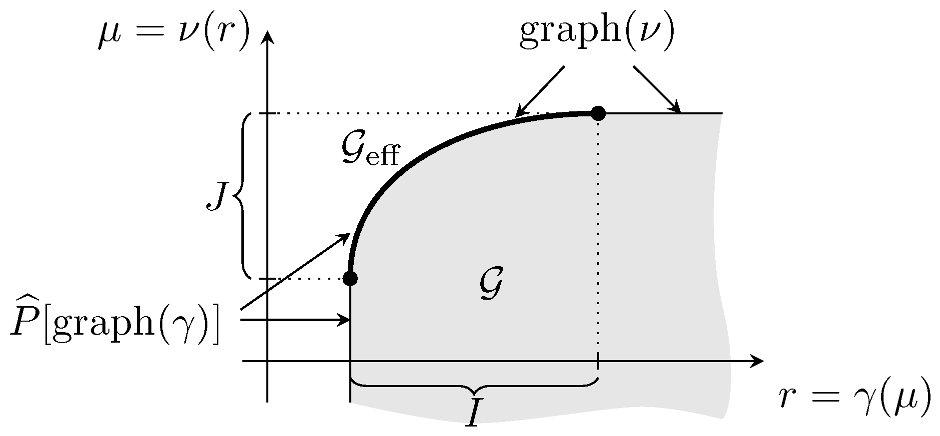
A typical situation of Theorem 2 may be viewed in Figure 1, where I and J are both bounded and closed. Notice that, in this example, the graph of ${\nu }_{\mid I}$ and $graph\left(\nu \right)$ do not coincide.

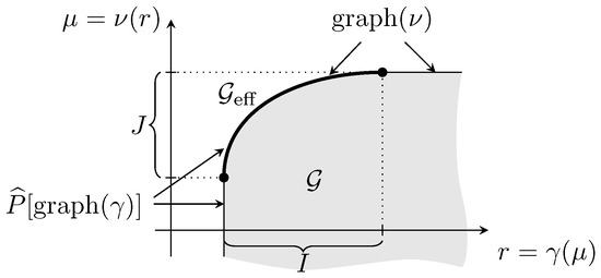
Figure 1. ${\mathcal{G}}_{\mathrm{eff}}$ as graph of ${\gamma }_{\mid J}$ and ${\nu }_{\mid I}$ (see (Maier-Paape et al. 2023), fig. 2.2).

However, the intervals I and J may also be open, or half-open to either side (cf. Figure 2).

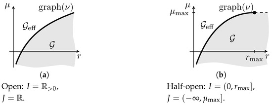
Figure 2. ${\mathcal{G}}_{\mathrm{eff}}$ examples for a risk function $\mathfrak{r}$ with non-negative values (see (Maier-Paape et al. 2023), fig. 2.4).

With the “endpoints” of I and J being included or not, it appears that there should be at least sixteen different possibilities for the tuple $(I,J)$, and thus for ${\mathcal{G}}_{\mathrm{eff}}$. In reality, however, we will see in Corollary 4(e) that there are only four different options for ${\mathcal{G}}_{\mathrm{eff}}$ concerning the endpoints of I and J.

4. Efficient Portfolios within the General Framework of Portfolio Theory for Scalar Risk

Having investigated the efficient frontier in detail in Section 3, we now turn our focus to related efficient portfolios granted within the GFPT.

Theorem 3 

(Continuous efficient portfolio map; Maier-Paape et al. 2023, Theorem 2.79). Assume, for a set $A\subset {\mathbb{R}}^{M+1}$ of admissible portfolios, as well as for extended-valued risk and utility functions $\mathfrak{r}$ and $\mathfrak{u}$, that Assumption 4 holds. Suppose additionally that either $\mathfrak{u}$ is strictly concave on $dom\left(\mathfrak{u}\right)\subset A$, i.e., (u2s) in Assumption 2 holds, or $\mathfrak{r}$ is strictly convex on $dom\left(\mathfrak{r}\right)\subset A$, i.e., (r2s) in Assumption 1 holds. Then, the following holds true:

(a)

Each point $(r,\mu )\in {\mathcal{G}}_{\mathrm{eff}}={\mathcal{G}}_{\mathrm{eff}}(\mathfrak{r},\mathfrak{u};A)$, with ${\mathcal{G}}_{\mathrm{eff}}$ from Definition 4, corresponds to a unique efficient portfolio $X(r,\mu )\in A$ realizing the risk–utility values $(r,\mu )$.

(b)

The mapping

$$\begin{array}{cc}\hfill X:{\mathcal{G}}_{\mathrm{eff}}(\mathfrak{r},\mathfrak{u};A)& \to A\subset {\mathbb{R}}^{M+1},\hfill \\ \hfill (r,\mu )& \mapsto X(r,\mu ),\hfill \end{array}$$

is injective and continuous (one-sided continuous at finite endpoint(s) of ${\mathcal{G}}_{\mathrm{eff}}$). Therefore, the efficient portfolios lie on a continuous curve with no self-intersections. Furthermore, X is surjective onto the set of efficient portfolios in A.

(c)

Moreover, efficient portfolios have the continuous representations

$$x^{*}:r\mapsto x^{*}\left(r\right):=X(r,\nu \left(r\right)),r\in I,$$

(16)

and

$$y^{*}:\mu \mapsto y^{*}\left(\mu \right):=X(\gamma \left(\mu \right),\mu ),\mu \in J,$$

(17)

on intervals I and J defined in (13) and (14), respectively, where ν and γ are defined in (12) and (11).

Under the standing assumptions from Assumption 4, a direct consequence of Definition 4 is that the existence part in Theorem 3(a) is obvious. Uniqueness, however, follows from the strictness conditions of either $\mathfrak{u}$ or $\mathfrak{r}$.

Apparently, with Theorem 3, all efficient portfolios lie on a (path-connected) curve. This is essential for applications. It guarantees that little changes in $\mu \in J$ for the minimum risk optimization problem

$$\underset{x\in A}{min}\mathfrak{r}\left(x\right)\mathrm{subject}\mathrm{to}\mathfrak{u}\left(x\right)\ge \mu$$

(18)

lead to minor adaptions of the corresponding efficient portfolio solving (18) (cf. the representation (17), as well as the continuity of ${\gamma }_{\mid J}$ due to Theorem 2(a), and the continuity of X on ${\mathcal{G}}_{\mathrm{eff}}$ due to Theorem 3(b)). Thus, fund managers are able to adjust such strategies continuously. A similar remark applies to the efficient portfolios solving the maximum utility optimization problem for given $r\in I$, i.e.,

$$\underset{x\in A}{max}\mathfrak{u}\left(x\right)\mathrm{subject}\mathrm{to}\mathfrak{r}\left(x\right)\le r.$$

(19)

For illustration purposes, we give a simple example.

Example 2 

(Case of an efficient pure bond portfolio realizing minimum risk). Let $A,\mathfrak{r}$ and $\mathfrak{u}$ satisfy the assumptions of Theorem 3. Furthermore, $\mathfrak{r}$ should satisfy (r1n) from Assumption 1 and A should contain only portfolios with unit initial cost (see Definition A4 in Appendix A). Then, the set $\{x\in A:\mathfrak{r}(x)\le 0\}$ contains exactly one element, which is the pure bond portfolio $x_{bond}^{★}:={(1,{\widehat{0}}^{\top })}^{\top }\in A\subset {\mathbb{R}}^{M+1}$ with a minimal possible risk value $r_{bond}:=\mathfrak{r}\left(x_{bond}^{★}\right)=0$. In the case where its utility value ${\mu }_{bond}:=\mathfrak{u}\left(x_{bond}^{★}\right)$ is finite, then $x_{bond}^{★}$ is in fact an efficient portfolio, so that $(r_{bond},{\mu }_{bond})\in {\mathcal{G}}_{\mathrm{eff}}(\mathfrak{r},\mathfrak{u};A)$. Hence, $X(r_{bond},{\mu }_{bond})=x_{bond}^{★}$.

Following on from Proposition 2(c), we briefly explain here how to find an efficient portfolio for a given point $(r,\mu )\in \mathcal{G}$, whose risk is not higher than r and whose utility is not lower than $\mu$.

Lemma 1 

(Construction of an efficient portfolio). Let the situation of Proposition 2 be given. Furthermore, let $\overline{x}\in dom\left(\mathfrak{r}\right)\cap dom\left(\mathfrak{u}\right)$. Then, there exists an efficient portfolio $x^{★}\in A$, such that

$$\mathfrak{r}\left(x^{★}\right)\le \mathfrak{r}\left(\overline{x}\right)\mathit{and}\mathfrak{u}\left(x^{★}\right)\ge \mathfrak{u}\left(\overline{x}\right).$$

Proof. 

The proof of this lemma goes back to ideas provided in the proof of Maier-Paape et al. (2023), Proposition 2.68(c). Because of its importance, we here give the following quick argument: Since $\overline{x}\in dom\left(\mathfrak{r}\right)\cap dom\left(\mathfrak{u}\right)$, $(\overline{r},\overline{\mu }):=(\mathfrak{r}\left(\overline{x}\right),\mathfrak{u}\left(\overline{x}\right))\in \mathcal{G}=\mathcal{G}(\mathfrak{r},\mathfrak{u};A)$ follows. Then, by lowering r and increasing $\mu$, while staying in $\mathcal{G}$, one finally reaches a point $(r^{★},{\mu }^{★})\in \partial \mathcal{G}\subset \mathcal{G}$, which cannot be improved, so $(r^{★},{\mu }^{★})\in {\mathcal{G}}_{\mathrm{eff}}={\mathcal{G}}_{\mathrm{eff}}(\mathfrak{r},\mathfrak{u};A)$ results. This is a consequence of $\nu \left(r\right)<\infty$ for all $r\in \mathbb{R}$ and $\gamma \left(\mu \right)>-\infty$ for all $\mu \in \mathbb{R}$, according to Proposition 2(b). By construction, $r^{★}\le \overline{r}$ and ${\mu }^{★}\ge \overline{\mu }$ is valid, and, since $(r^{★},{\mu }^{★})\in {\mathcal{G}}_{\mathrm{eff}}$, there exists an efficient portfolio $x^{★}\in A$ such that

$$\mathfrak{r}\left(x^{★}\right)=r^{★}\le \overline{r}=\mathfrak{r}\left(\overline{x}\right)\mathrm{and}\mathfrak{u}\left(x^{★}\right)={\mu }^{★}\ge \overline{\mu }=\mathfrak{u}\left(\overline{x}\right),$$

as claimed. □

5. Endpoints of the Efficient Frontier within the General Framework of Portfolio Theory for Scalar Risk

Apparently, the sets I and J, defined in Corollary 1, are of great interest for this theory, since they may be used for parameterizations of the efficient frontier (see Theorem 2) and the efficient portfolios (cf. (16) and (17)). In this section, we investigate the “endpoints” of these intervals (cf. Corollary 3).

Definition 5 

(“Endpoints” of I and J; Maier-Paape et al. 2023, Definition 2.81). For the intervals $I=I(\mathfrak{r},\mathfrak{u};A)$ and $J=J(\mathfrak{r},\mathfrak{u};A)$, defined in (13) and (14) as projections of ${\mathcal{G}}_{\mathrm{eff}}=$${\mathcal{G}}_{\mathrm{eff}}(\mathfrak{r},\mathfrak{u};A)$ to the axes, we set:

$$\begin{array}{cc}\hfill & r_{min}:=infI=\underset{(r,\mu )\in {\mathcal{G}}_{\mathrm{eff}}}{inf}\left\{r\right\}=inf[dom\left(\nu \right)\cap range\left(\gamma \right)],\hfill \\ \hfill & r_{max}:=supI=\underset{(r,\mu )\in {\mathcal{G}}_{\mathrm{eff}}}{sup}\left\{r\right\}=sup[dom\left(\nu \right)\cap range\left(\gamma \right)],\hfill \\ \hfill & {\mu }_{min}:=infJ=\underset{(r,\mu )\in {\mathcal{G}}_{\mathrm{eff}}}{inf}\left\{\mu \right\}=inf[dom\left(\gamma \right)\cap range\left(\nu \right)],\hfill \\ \hfill & {\mu }_{max}:=supJ=\underset{(r,\mu )\in {\mathcal{G}}_{\mathrm{eff}}}{sup}\left\{\mu \right\}=sup[dom\left(\gamma \right)\cap range\left(\nu \right)].\hfill \end{array}$$

The above defined values may or may not lie in $\mathbb{R}$, because I or J might be unbounded. Notice that all above representations are evident using the definitions in (13) and (14), as well as Corollary 1(a) and (b). The next proposition, however, is a bit more involved (cf. Maier-Paape et al. 2023).

Proposition 3 

(Alternative representations of “endpoints” of I and J; Maier-Paape et al. 2023, Proposition 2.82). Assume, for a set $A\subset {\mathbb{R}}^{M+1}$ of admissible portfolios, as well as extended-valued risk and utility functions $\mathfrak{r}$ and $\mathfrak{u}$, that Assumption 4 holds. Then, using $\mathcal{B}:=dom\left(\mathfrak{u}\right)\cap dom\left(\mathfrak{r}\right)\subset A$, the following holds true:

$$\begin{array}{cc}\hfill r_{min}& =\underset{x\in \mathcal{B}}{inf}\left\{\mathfrak{r}\left(x\right)\right\}=inf\{\mathfrak{r}\left(x\right):\mathfrak{u}\left(x\right)>-\infty ,x\in A\}<+\infty ,\hfill \end{array}$$

(20)

$$\begin{array}{cc}\hfill {\mu }_{max}& =\underset{x\in \mathcal{B}}{sup}\left\{\mathfrak{u}\left(x\right)\right\}=sup\{\mathfrak{u}\left(x\right):\mathfrak{r}\left(x\right)<+\infty ,x\in A\}>-\infty ,\hfill \end{array}$$

(21)

$$\begin{array}{cc}\hfill {\mu }_{min}& =\underset{r\searrow r_{min}}{lim}sup\{\mathfrak{u}\left(x\right):\mathfrak{r}\left(x\right)\le r,x\in A\}\le {\mu }_{max},\hfill \end{array}$$

(22)

$$\begin{array}{cc}\hfill r_{max}& =\underset{\mu \nearrow {\mu }_{max}}{lim}inf\{\mathfrak{r}\left(x\right):\mathfrak{u}\left(x\right)\ge \mu ,x\in A\}\ge r_{min}.\hfill \end{array}$$

(23)

With these representations at hand, and using some technical argumentation, it is possible to show several nontrivial relations between $r_{min}$ and ${\mu }_{min}$ on the one hand, and between $r_{max}$ and ${\mu }_{max}$ on the other hand (see below).

Corollary 4 

(“Endpoint” properties; Maier-Paape et al. 2023, Corollary 2.83). In the situation of Proposition 3 with $I=I(\mathfrak{r},\mathfrak{u};A)$ and $J=J(\mathfrak{r},\mathfrak{u};A)$, defined in (13) and (14), we have:

(a)

$r_{min}\in I$, if and only if ${\mu }_{min}\in J$.

(b)

If $r_{min}\in I$, then ${\mu }_{min}=\nu \left(r_{min}\right)$ and $\gamma \left({\mu }_{min}\right)=r_{min}$.

(c)

$r_{max}\in I$, if and only if ${\mu }_{max}\in J$.

(d)

If ${\mu }_{max}\in J$, then $r_{max}=\gamma \left({\mu }_{max}\right)$ and $\nu \left(r_{max}\right)={\mu }_{max}$.

(e)

 

(i)

If $r_{min}\in I$ and ${\mu }_{max}\in J$, then $I=\left[r_{min},r_{max}\right]$ and $J=\left[{\mu }_{min},{\mu }_{max}\right]$.

(ii)

If $r_{min}\in I$ and ${\mu }_{max}\notin J$, then $I=\left[r_{min},\infty \right)$ and $J=\left[{\mu }_{min},{\mu }_{max}\right)$.

(iii)

If $r_{min}\notin I$ and ${\mu }_{max}\in J$, then $I=\left(r_{min},r_{max}\right]$ and $J=\left(-\infty ,{\mu }_{max}\right]$.

(iv)

If $r_{\min }\notin I$ and ${\mu }_{max}\notin J$, then $I=\left(r_{min},\infty \right)$ and $J=\left(-\infty ,{\mu }_{max}\right)$.

In particular, as already noted at the end of Section 3, according to Corollary 4(e), we obtain only four different possibilities for the tuple $(I,J)$, and thus for ${\mathcal{G}}_{\mathrm{eff}}$.

Thus, Maier-Paape et al. (2023) have examined the behavior and properties of $\gamma$ and $\nu$ on J and I, respectively, (cf., e.g., Theorem 2) as well as the intervals J and I themselves (cf., e.g., Corollary 4) in detail. We will conclude with a brief look at how $\gamma$ and $\nu$ behave outside J and I, respectively (cf. Figure 1 for an illustration). Although the respective graphs outside J and I do not contribute to the efficient frontier, the behavior of $\gamma$ and $\nu$ there is often of technical value.

Lemma 2 

(Behavior of $\gamma$ or $\nu$ outside of J or I). In the situation of Proposition 3, with $I=I(\mathfrak{r},\mathfrak{u};A)$ and $J=J(\mathfrak{r},\mathfrak{u};A)$ defined in (13) and (14), the following holds:

(a)

If ${\mu }_{max}\in J$, then $r_{max}\in I$ and $\nu \left(r\right)={\mu }_{max}$ for all $r\ge r_{max}$.

(b)

If $r_{min}\in I$, then ${\mu }_{min}\in J$ and $\gamma \left(\mu \right)=r_{min}$ for all $\mu \le {\mu }_{min}$.

(c)

 

(i)

If $r_{min}\in I$, then $\nu \left(r\right)=-\infty$ for all $r<r_{min}$.

(ii)

If $r_{min}\notin I$ and $r_{min}\in \mathbb{R}$, then $\nu \left(r\right)=-\infty$ for all $r\le r_{min}$.

(d)

 

(i)

If ${\mu }_{max}\in J$, then $\gamma \left(\mu \right)=\infty$ for all $\mu >{\mu }_{max}$.

(ii)

If ${\mu }_{max}\notin J$ and ${\mu }_{max}\in \mathbb{R}$, then $\gamma \left(\mu \right)=\infty$ for all $\mu \ge {\mu }_{max}$.

Proof. 

We only have to consider (a) and (c) because (b) and (d) are symmetric statements.

ad(a). Let ${\mu }_{max}\in J$. Then, by Corollary 4(c), (d), $r_{max}\in I$ with $\nu \left(r_{max}\right)={\mu }_{max}$ follows. Furthermore, since

$$\nu \left(r\right)\stackrel{\left(12\right)}{=}sup\{\mathfrak{u}\left(x\right):\mathfrak{r}\left(x\right)\le r,x\in A\}\le sup\{\mathfrak{u}\left(x\right):\mathfrak{r}\left(x\right)<\infty ,x\in A\}\stackrel{\left(21\right)}{=}{\mu }_{max}$$

holds, and $\nu$ is increasing by Proposition 2(b), we obtain $\nu \left(r\right)={\mu }_{max}$ for all $r\ge r_{max}$.

ad(c). These assertions can be shown straight forwardly with the help of Lemma 1 by using the definitions of $r_{min}$ in (20) and of $\nu$ in (12). □

6. Generalizations of the General Framework of Portfolio Theory for Vector Risk

In this section, the risk function is assumed to be vector-valued, while the utility function remains to be scalar and, as before, $A\subset {\mathbb{R}}^{M+1}$ is a set of admissible portfolios. The results of the General Framework of Portfolio Theory (GFPT) for this case are taken from Maier-Paape et al. (2023, chap. 3). However, in contrast to the theory developed there for $d\ge 2$ dimensional risk vectors, we restrain ourselves here for simplicity and visualization reasons to $d=2$.

Assumption 5 

(Conditions on the vector risk functions; see Assumption 1 and Maier-Paape et al. 2023, Assumption 3.1). Consider a vector risk function $\mathfrak{r}=\left({\mathfrak{r}}_1,{\mathfrak{r}}_2\right):A\to$${(\mathbb{R}\cup \{+\infty \})}^2$, with lower semi-continuous components ${\mathfrak{r}}_1$ and ${\mathfrak{r}}_2$, where $A\subset {\mathbb{R}}^{M+1}$ is a set of admissible portfolios according to Definition 2. We say that:

(a)

$\mathfrak{r}$ satisfies one (or more) of the conditions (r1), (r1n), or (r2) if ${\mathfrak{r}}_1$ and ${\mathfrak{r}}_2$ satisfy (r1), (r1n), or (r2) from Assumption 1, respectively;

(b)

$\mathfrak{r}$ satisfies (r2s) if ${\mathfrak{r}}_1$ or ${\mathfrak{r}}_2$ satisfies (r2s) from Assumption 1.

In the following we simplify notation by using ≤ and ≥ componentwise; i.e., for two vectors $v=(v_1,v_2),w=(w_1,w_2)\in {\mathbb{R}}^2$, we have $v\le w$, if and only if $v_i\le w_i$ for $i=1,2$ (analogously for the other operator).

Remark 2 

(Risk–utility as row vectors; see Maier-Paape et al. 2023, Remark 3.3). Here, and in the following, it is convenient to have risk vectors $r=(r_1,r_2)\in {\mathbb{R}}^2$ as row vectors. Similarly, the risk–utility vectors $(r,\mu )\in {\mathbb{R}}^2\times \mathbb{R}={\mathbb{R}}^3$ are assumed to be row vectors, which is in contrast to our portfolio vectors $x\in A$, which are always column vectors.

Similarly to Assumption 3, for the scalar risk case, we rely here on compactness assumptions as well.

Assumption 6 

(Compact level sets in vector risk case; see Maier-Paape et al. 2023, Assumption 3.4). We assume for a vector-valued risk function $\mathfrak{r}:A\to {\left(\mathbb{R}\cup \{+\infty \}\right)}^2$, as in Assumption 5, and a scalar-valued utility function $\mathfrak{u}:A\to \mathbb{R}\cup \{-\infty \}$, as in Assumption 2, that:

(a)

$dom\left(\mathfrak{u}\right)\cap dom\left(\mathfrak{r}\right)\ne \varnothing$;

(b)

For all $(r,\mu )\in {\mathbb{R}}^3$, the sets

$${\mathcal{B}}_A^{\left(2d\right)}(\mathfrak{r}\le r;\mathfrak{u}\ge \mu ):=\{x\in A:\mathfrak{r}\left(x\right)\le r\mathrm{and}\mathfrak{u}\left(x\right)\ge \mu \}$$

(24)

are compact.

The next proposition lifts Proposition 1 to the vector risk case.

Proposition 4 

(Properties of ${\mathcal{G}}^{\left(2d\right)}={\mathcal{G}}^{\left(2d\right)}(\mathfrak{r},\mathfrak{u};A)$; cf. Maier-Paape et al. 2023, Proposition 3.6). Assume that $A\subset {\mathbb{R}}^{M+1}$ is a set of admissible portfolios, as in Definition 2. In addition, assume that the vector risk function $\mathfrak{r}$ satisfies (r2) in Assumption 5, and the utility function $\mathfrak{u}$ satisfies (u2) in Assumption 2. We then have:

(a)

The set of valid risk and utility values

$${\mathcal{G}}^{\left(2d\right)}={\mathcal{G}}^{\left(2d\right)}(\mathfrak{r},\mathfrak{u};A):=\left\{(r,\mu )\in {\mathbb{R}}^3:\exists x\in A\mathrm{s}.\mathrm{t}.\mathfrak{r}\left(x\right)\le r\mathrm{and}\mathfrak{u}\left(x\right)\ge \mu \right\}\subset {\mathbb{R}}^3$$

(25)

is convex.

(b)

$(r,\mu )\in {\mathcal{G}}^{\left(2d\right)}(\mathfrak{r},\mathfrak{u};A)$ implies that, for any $\left(k,k_0\right)\in {\mathbb{R}}_{\ge 0}^2\times {\mathbb{R}}_{\ge 0}$, we have $(r+k,\mu )\in {\mathcal{G}}^{\left(2d\right)}(\mathfrak{r},\mathfrak{u};A)$ and $\left(r,\mu -k_0\right)\in {\mathcal{G}}^{\left(2d\right)}(\mathfrak{r},\mathfrak{u};A)$.

(c)

Assume furthermore that Assumption 6(b) holds. Then, ${\mathcal{G}}^{\left(2d\right)}(\mathfrak{r},\mathfrak{u};A)$ is closed.

With all that notation at hand, we can now define efficient portfolios and the efficient frontier in the vector risk case.

Definition 6 

(Efficient portfolios in vector risk case; see Maier-Paape et al. 2023, Definition 3.7). We say that a portfolio $x^{★}\in A$ with finite risk and utility values is Pareto efficient (for given vector risk function $\mathfrak{r}$, scalar utility function $\mathfrak{u}$, and admissible portfolios A), provided that there does not exist any portfolio $x^{\prime }\in A$ such that either

$$\left[\mathfrak{r}\left(x^{\prime }\right)\le \mathfrak{r}\left(x^{★}\right)\mathrm{and}\mathfrak{u}\left(x^{\prime }\right)>\mathfrak{u}\left(x^{★}\right)\right]$$

or

$$\left[\mathfrak{r}\left(x^{\prime }\right)\le \mathfrak{r}\left(x^{★}\right),\mathfrak{r}\left(x^{\prime }\right)\ne \mathfrak{r}\left(x^{★}\right)\mathrm{and}\mathfrak{u}\left(x^{\prime }\right)\ge \mathfrak{u}\left(x^{★}\right)\right]$$

holds.

For better understanding, it is worthwhile to compare Definition 6 with the one of the scalar risk case; see Definition 3.

Definition 7 

(Efficient frontier in vector risk case; see Definition 4 and Maier-Paape et al. 2023, Definition 3.8). We call the set of (risk–utility) images of all efficient portfolios in the three-dimensional risk–utility space the efficient frontier, and denote it by ${\mathcal{G}}_{\mathrm{eff}}^{\left(2d\right)}={\mathcal{G}}_{\mathrm{eff}}^{\left(2d\right)}(\mathfrak{r},\mathfrak{u};A)$.

Similarly to some of the properties of the efficient frontier for the scalar risk case given in Theorem 1, we obtain the following for the vector risk case.

Theorem 4 

(Efficient frontier properties in vector risk case; confer Theorem 3.9 in Maier-Paape et al. 2023). Efficient portfolios represented in the three-dimensional risk–utility space are all located on the boundary $\partial {\mathcal{G}}^{\left(2d\right)}=\partial {\mathcal{G}}^{\left(2d\right)}(\mathfrak{r},\mathfrak{u};A)$ of the set ${\mathcal{G}}^{\left(2d\right)}(\mathfrak{r},\mathfrak{u};A)$. In case the boundary of ${\mathcal{G}}^{\left(2d\right)}(\mathfrak{r},\mathfrak{u};A)$ contains a line segment parallel to any of the three coordinate axes, on such a line segment lies, at most, one efficient portfolio.

The analog of the “standing” Assumption 4 for the scalar risk case is given for the vector risk case next.

Assumption 7 

(Standing assumptions for efficient trade-off in vector risk case; see Maier-Paape et al. 2023, Assumption 3.11). We assume the following properties:

(a)

$A\subset {\mathbb{R}}^{M+1}$ is a set of admissible portfolios, according to Definition 2.

(b)

$\mathfrak{r}:A\to {(\mathbb{R}\cup \{+\infty \})}^2$ is a lower semi-continuous extended-valued vector risk function satisfying (r2) in Assumption 5.

(c)

$\mathfrak{u}:A\to \mathbb{R}\cup \{-\infty \}$ is an upper semi-continuous extended-valued scalar utility function satisfying (u2) in Assumption 2.

(d)

Assumption 6 concerning compact level sets holds for $A,\mathfrak{r}$, and $\mathfrak{u}$.

From now on, we use the following notations for risk values $r=(r_1,r_2)\in {\mathbb{R}}^2$:

$$r_2=:{\widehat{r}}^1\in {\widehat{\mathbb{R}}}_1^2:=\mathbb{R}\mathrm{and}{r}_1=:{\widehat{r}}^2\in {\widehat{\mathbb{R}}}_2^2:=\mathbb{R},$$

(26)

i.e., we have $r=(r_1,{\widehat{r}}^1)=({\widehat{r}}^2,r_2)$.

While we only had two auxiliary functions $\gamma$ and $\nu$ for the scalar risk case (see Proposition 2), we now obtain three auxiliary functions for two-dimensional vector risk.

Proposition 5 

(Auxiliary functions related to the efficient frontier in vector risk case; see Maier-Paape et al. 2023, Proposition 3.12). Assume, for a set $A\subset {\mathbb{R}}^{M+1}$ of admissible portfolios, as well as for extended-valued vector risk and scalar utility functions $\mathfrak{r}$ and $\mathfrak{u}$, that Assumption 7 holds. Then, the following holds true:

(a)

${\mathcal{G}}^{\left(2d\right)}(\mathfrak{r},\mathfrak{u};A)\ne \varnothing$.

(b)

The functions $\nu :{\mathbb{R}}^2\to \mathbb{R}\cup \{-\infty \}$, defined by

$$\begin{array}{cc}\hfill \nu \left(r\right)& :=sup\left\{\mu :(r,\mu )\in {\mathcal{G}}^{\left(2d\right)}(\mathfrak{r},\mathfrak{u};A)\subset {\mathbb{R}}^3\right\}\hfill \\ \hfill & =sup\{\mathfrak{u}\left(x\right):\mathfrak{r}\left(x\right)\le r,x\in A\},r\in {\mathbb{R}}^2,\hfill \end{array}$$

(27)

and ${\gamma }_k:{\mathbb{R}}^2\to \mathbb{R}\cup \{+\infty \}$, defined by

$$\begin{array}{cc}\hfill {\gamma }_k\left({\widehat{r}}^k,\mu \right)& :=inf\left\{r_k:(r,\mu )\in {\mathcal{G}}^{\left(2d\right)}(\mathfrak{r},\mathfrak{u};A)\subset {\mathbb{R}}^3\right\}\hfill \\ \hfill & =inf\left\{{\mathfrak{r}}_k\left(x\right):\mathfrak{u}\left(x\right)\ge \mu ,{\widehat{\mathfrak{r}}}^k\left(x\right)\le {\widehat{r}}^k,x\in A\right\},\left({\widehat{r}}^k,\mu \right)\in {\mathbb{R}}^2,\hfill \end{array}$$

(28)

for $k=1,2$, are well-defined extended-valued functions. Moreover, the function ${\gamma }_k$ is decreasing in ${\widehat{r}}^k$, increasing in μ, and lower semi-continuous as well as proper convex. The function ν is increasing (coordinate-wise), upper semi-continuous, and proper concave.

(c)

${\mathcal{G}}_{\mathrm{eff}}^{\left(2d\right)}(\mathfrak{r},\mathfrak{u};A)\ne \varnothing$.

In the following, using the definitions in (26), we define the projections

$$\mathrm{Pro}{\mathrm{j}}_{{\widehat{\mathbb{R}}}_k^2\times \mathbb{R}}:{\mathbb{R}}^3\to {\widehat{\mathbb{R}}}_k^2\times \mathbb{R}\cong {\mathbb{R}}^2,\mathrm{Pro}{\mathrm{j}}_{{\widehat{\mathbb{R}}}_k^2\times \mathbb{R}}(r,\mu ):=({\widehat{r}}^k,\mu ),$$

(29)

for $k=1,2$ and

$$\mathrm{Pro}{\mathrm{j}}_{{\mathbb{R}}^2}:{\mathbb{R}}^3\to {\mathbb{R}}^2,\mathrm{Pro}{\mathrm{j}}_{{\mathbb{R}}^2}(r,\mu ):=r,$$

(30)

as well as some kind of permutation mappings

$${\widehat{\mathrm{P}}}_k:{\mathbb{R}}^3\to {\mathbb{R}}^3,{\widehat{\mathrm{P}}}_k\left({\widehat{r}}^k,\mu ,r_k\right):=(r,\mu ),$$

(31)

for $k=1,2$.

We now shift our focus to projections of the efficient frontier ${\mathcal{G}}_{\mathrm{eff}}^{\left(2d\right)}$ from the three-dimensional risk–utility space to planes built by two of the three variables $(r_1,r_2,\mu )$. This result is along the lines of Corollary 1 and Theorem 2(c) for the scalar risk case. In particular, the definitions in (32) and (35) below should be compared with the definitions of the sets I and J in (13) and (14).

Theorem 5 

(Representation of efficient frontier in vector risk case; see Theorem 3.14 in Maier-Paape et al. 2023). Assume, for a set $A\subset {\mathbb{R}}^{M+1}$ of admissible portfolios, that the vector risk function $\mathfrak{r}:A\to {(\mathbb{R}\cup \{+\infty \})}^2$ and the scalar utility function $\mathfrak{u}:A\to \mathbb{R}\cup \{-\infty \}$ satisfy Assumption 7. Then, the following holds true:

(a)

Setting

$$\begin{array}{cc}\hfill N=N(\mathfrak{r},\mathfrak{u};A)& :={Proj}_{{\mathbb{R}}^2}\left({\mathcal{G}}_{\mathrm{eff}}^{\left(2d\right)}(\mathfrak{r},\mathfrak{u};A)\right)\hfill \\ \hfill & =\left\{r\in {\mathbb{R}}^2:\exists \mu \in \mathbb{R}\mathit{with}(r,\mu )\in {\mathcal{G}}_{\mathrm{eff}}^{\left(2d\right)}(\mathfrak{r},\mathfrak{u};A)\right\},\hfill \end{array}$$

(32)

we have

$$\begin{array}{cc}\hfill N& ={Proj}_{{\mathbb{R}}^2}\left(graph\left({\nu |}_{dom\left(\nu \right)}\right)\right)\cap \bigcap _{k=1}^2{Proj}_{{\mathbb{R}}^2}\left({\widehat{P}}_k\left[graph\left({\gamma }_k{|}_{dom\left({\gamma }_k\right)}\right)\right]\right)\hfill \\ \hfill & \subset {Proj}_{{\mathbb{R}}^2}\left(graph\left({\nu |}_{dom\left(\nu \right)}\right)\right)=dom\left(\nu \right)\hfill \end{array}$$

(33)

and

$${\mathcal{G}}_{\mathrm{eff}}^{\left(2d\right)}(\mathfrak{r},\mathfrak{u};A)=graph\left({\nu |}_N\right).$$

(34)

(b)

For arbitrary but fixed $k\in \{1,2\}$, we set

$$\begin{array}{cc}\hfill M_k& =M_k(\mathfrak{r},\mathfrak{u};A):={Proj}_{{\widehat{\mathbb{R}}}_k^2\times \mathbb{R}}\left({\mathcal{G}}_{\mathrm{eff}}^{\left(2d\right)}(\mathfrak{r},\mathfrak{u};A)\right)\hfill \\ \hfill & =\left\{({\widehat{r}}^k,\mu ):\exists r_k\in \mathbb{R}\mathit{with}(r,\mu )\in {\mathcal{G}}_{\mathrm{eff}}^{\left(2d\right)}(\mathfrak{r},\mathfrak{u};A)\right\}.\hfill \end{array}$$

(35)

Then, we have

$$\begin{array}{cc}\hfill M_k& ={Proj}_{{\widehat{\mathbb{R}}}_k^2\times \mathbb{R}}\left(graph\left({\nu |}_{dom\left(\nu \right)}\right)\right)\cap \bigcap _{\ell =1}^2{Proj}_{{\widehat{\mathbb{R}}}_k^2\times \mathbb{R}}\left({\widehat{P}}_{\ell }\left[graph\left({\gamma }_{\ell }{|}_{dom\left({\gamma }_{\ell }\right)}\right)\right]\right)\hfill \\ \hfill & \subset {Proj}_{{\widehat{\mathbb{R}}}_k^2\times \mathbb{R}}\left({\widehat{P}}_k\left[graph\left({\gamma }_k{|}_{dom\left({\gamma }_k\right)}\right)\right]\right)=dom\left({\gamma }_k\right)\hfill \end{array}$$

and

$${\mathcal{G}}_{\mathrm{eff}}^{\left(2d\right)}(\mathfrak{r},\mathfrak{u};A)={\widehat{P}}_k\left[graph\left({\gamma }_k{|}_{M_k}\right)\right].$$

(36)

Note that Equations (34) and (36) provide representations of ${\mathcal{G}}_{\mathrm{eff}}^{\left(2d\right)}$ as graphs of the auxiliary functions $\nu ,{\gamma }_1$ and ${\gamma }_2$, respectively. In particular, we clearly obtain from (34) and (36) that

$${\mathcal{G}}_{\mathrm{eff}}^{\left(2d\right)}(\mathfrak{r},\mathfrak{u};A)=graph\left(\nu {|}_N\right)\cap {\widehat{\mathrm{P}}}_1\left[graph\left({\gamma }_1{|}_{M_1}\right)\right]\cap {\widehat{\mathrm{P}}}_2\left[graph\left({\gamma }_2{|}_{M_2}\right)\right],$$

(37)

but also that the following holds true using, e.g., (33) and (34):

$${\mathcal{G}}_{\mathrm{eff}}^{\left(2d\right)}(\mathfrak{r},\mathfrak{u};A)=graph\left({\nu |}_{dom\left(\nu \right)}\right)\cap {\widehat{P}}_1\left[graph\left({\gamma }_1{|}_{dom\left({\gamma }_1\right)}\right)\right]\cap {\widehat{P}}_2\left[graph\left({\gamma }_2{|}_{dom\left({\gamma }_2\right)}\right)\right].$$

This can also be seen in the following example which we provide for illustration purposes.

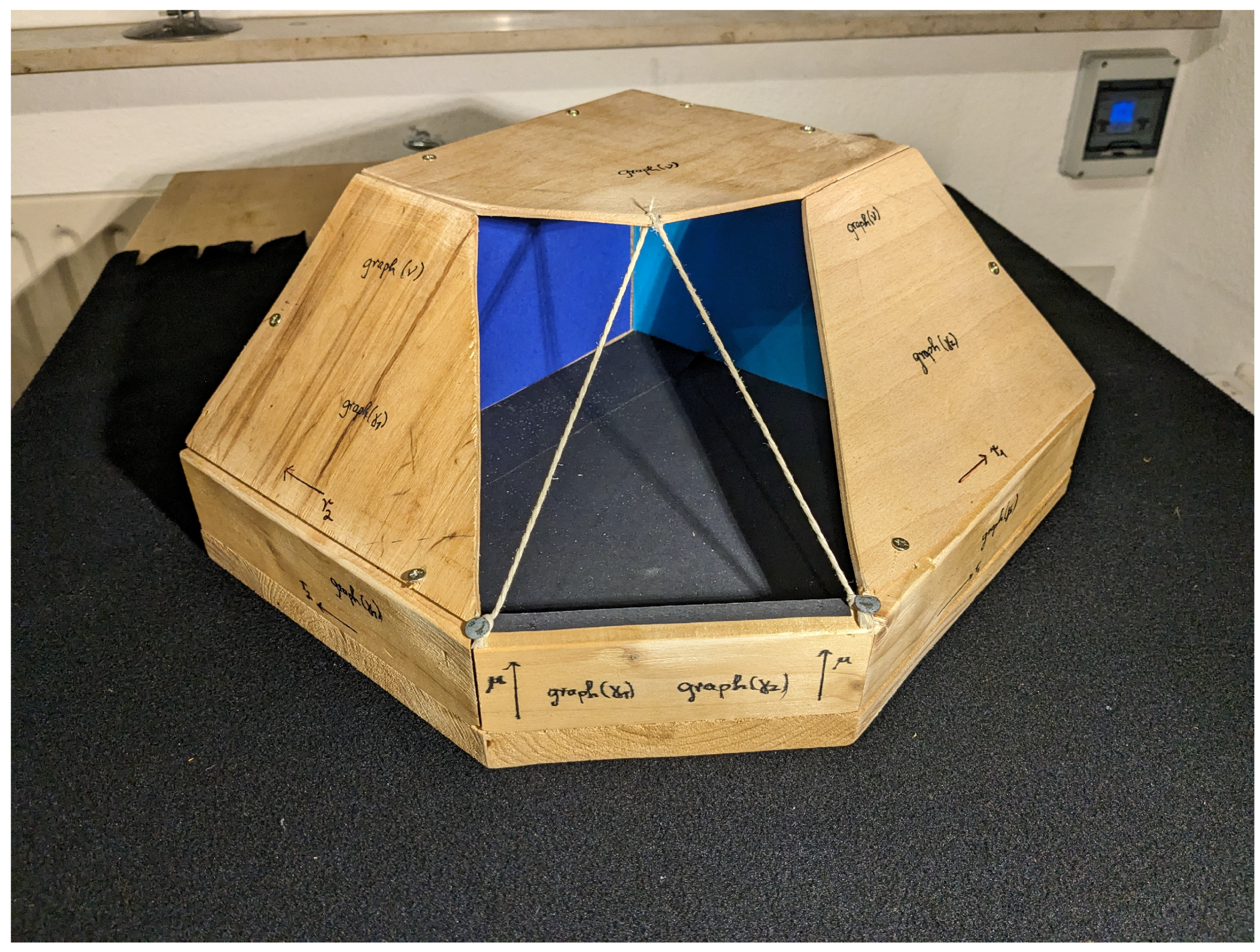
Example 3 

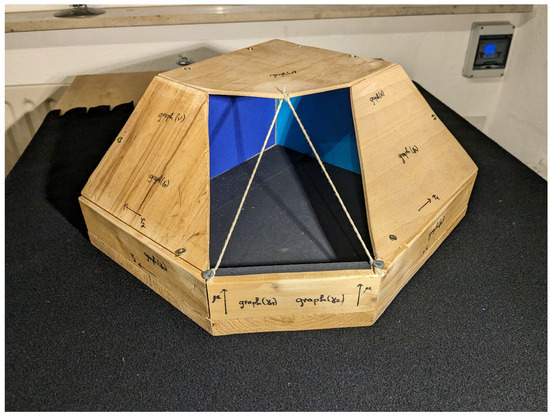
(Non-convex projections of ${\mathcal{G}}_{\mathrm{eff}}^{\left(2d\right)}$). In Figure 3, we see a wooden model to illustrate the boundary of a possible set ${\mathcal{G}}_{*}^{\left(2d\right)}:={\mathcal{G}}^{\left(2d\right)}({\mathfrak{r}}^{*},{\mathfrak{u}}^{*};A^{*})\subset {\mathbb{R}}^3$ and its efficient frontier ${\mathcal{G}}_{\mathrm{eff},*}^{\left(2d\right)}:={\mathcal{G}}_{\mathrm{eff}}^{\left(2d\right)}({\mathfrak{r}}^{*},{\mathfrak{u}}^{*};A^{*})$ for the vector risk case and some fixed risk and utility functions, ${\mathfrak{r}}^{*}$ and ${\mathfrak{u}}^{*}$, as well as a fixed set of possible admissible portfolios $A^{*}$ (whose specific forms are all irrelevant for now).

Figure 3. The efficient frontier ${\mathcal{G}}_{\mathrm{eff},*}^{\left(2d\right)}={\mathcal{G}}_{\mathrm{eff}}^{\left(2d\right)}({\mathfrak{r}}^{*},{\mathfrak{u}}^{*};A^{*})\subset {\mathbb{R}}^3$ is build by three transparent “cord” facets.

Of course, the black “ground plate” of the wooden model in Figure 3 is just there to hold the construction. The extensions of the side lines of the ground plate to the left and to the right should be viewed as $r_1$- and $r_2$-axis. Perpendicular to these axes and upwards directed is the μ-axis. Note that, e.g., the facets on top $\left(\nu =\mathrm{const}={\mu }_{max}^{*}:=sup\left\{\mu :(r,\mu )\in {\mathcal{G}}_{\mathrm{eff},*}^{\left(2d\right)}\right\}\right)$ or to the right and to the left have to be extended in $r_1$- and/or $r_2$-direction to $+\infty$ to obtain all of $\partial {\mathcal{G}}_{*}^{\left(2d\right)}:=\partial {\mathcal{G}}^{\left(2d\right)}({\mathfrak{r}}^{*},{\mathfrak{u}}^{*};A^{*})$. Similarly, the facets below are to be extended in μ-direction to $-\infty$. Also, the three transparent facets in front mimicked by a cord are part of $\partial {\mathcal{G}}_{*}^{\left(2d\right)}$. In fact, it is easy to see that only these three cord facets build ${\mathcal{G}}_{\mathrm{eff},*}^{\left(2d\right)}$. Moreover, the reader should be able to imagine, for this example, the set $N_{*}=N({\mathfrak{r}}^{*},{\mathfrak{u}}^{*};A^{*})$, i.e., the projection of ${\mathcal{G}}_{\mathrm{eff},*}^{\left(2d\right)}$ to the $(r_1,r_2)$-plane, which is a path-connected set, but $N_{*}$ is not convex in the case. This is remarkable because it is in contrast to the scalar risk case, where the projections of the efficient frontier to the axes, i.e., the sets I and J from (13) and (14) are always convex (see Corollary 3).

It should be furthermore noted that the representations of ${\mathcal{G}}_{\mathrm{eff}}^{\left(2d\right)}={\mathcal{G}}_{\mathrm{eff}}^{\left(2d\right)}(\mathfrak{r},\mathfrak{u};A)$ in (34) and (36) are an analog of Theorem 2(c) for the vector risk case. An analog of Theorem 2(b) for the vector risk case holds as well (see (38) and (39) below). However, continuity of ${\nu |}_N,{\gamma }_1{|}_{M_1}$ and ${\gamma }_2{|}_{M_2}$ is no longer granted unconditionally, although, for scalar risk, this was no problem (see Theorem 2(a)).

In consensus with definition (26), in the following, we use the convention that ${\widehat{r}}^k$ followed by $r_k$ is to be interpreted as a completed vector in ${\mathbb{R}}^2$, i.e.,

$$({\widehat{r}}^k,r_k):=(r_1,r_2)=r\in {\mathbb{R}}^2$$

for $k=1,2$.

Theorem 6 

(Representation of efficient frontier 2 in the vector risk case; see Maier-Paape et al. 2023, Corollary 3.15). Under the same assumptions as in Theorem 5, the following holds true:

(a)

$\nu :N\to \mathbb{R}$ is strictly increasing in each component; ${\gamma }_k:M_k\to \mathbb{R}$ is strictly increasing in μ and strictly decreasing in ${\widehat{r}}_k$ (coordinate-wise) for $k=1,2$.

(b)

${\gamma }_k:M_k\to \mathbb{R},k=1,2$ and $\nu :N\to \mathbb{R}$ are $\left(\mathit{for}\mathit{fixed}{\widehat{r}}^k\in {\widehat{\mathbb{R}}}_k^2\right)$ inverse to each other in the following sense:

$$\begin{array}{cc}\hfill {\gamma }_k\left({\widehat{r}}^k,\nu ({\widehat{r}}^k,r_k)\right)& =r_k\mathit{for}\mathit{all}r=({\widehat{r}}^k,r_k)\in N\subset dom\left(\nu \right),\hfill \\ \hfill \nu \left({\widehat{r}}^k,{\gamma }_k({\widehat{r}}^k,\mu )\right)& =\mu \mathit{for}\mathit{all}({\widehat{r}}^k,\mu )\in M_k\subset dom\left({\gamma }_k\right).\hfill \end{array}$$

(38)

(c)

${\gamma }_1:M_1\to \mathbb{R}$ and ${\gamma }_2:M_2\to \mathbb{R}$ are (for fixed $\mu \in \mathbb{R}$) inverse to each other in the following sense:

$$\begin{array}{cc}\hfill {\gamma }_2({\gamma }_1(r_2,\mu ),\mu )& =r_2\mathit{for}\mathit{all}(r_2,\mu )=({\widehat{r}}^1,\mu )\in M_1\subset dom\left({\gamma }_1\right),\hfill \\ \hfill {\gamma }_1({\gamma }_2(r_1,\mu ),\mu )& =r_1\mathit{for}\mathit{all}(r_1,\mu )=({\widehat{r}}^2,\mu )\in M_2\subset dom\left({\gamma }_2\right).\hfill \end{array}$$

(39)

Remark 3 

(Continuity of $\nu$ and ${\gamma }_k$ in the interior of their domains). As provided in Proposition 5, ν is upper semi-continuous and concave, and ${\gamma }_k$ is lower semi-continuous and convex for $k=1,2$. At least in the (relative) interior of their domains, both ν and ${\gamma }_k$ are even continuous (cf. Rockafellar 1972, Theorem 10.1). Nevertheless, discontinuities on the boundary are possible (see Maier-Paape et al. 2023, Example 3.16, for a counterexample to continuity at the boundary).

Path-connectedness of the efficient frontier in the scalar risk case was already not completely obvious (cf. Corollary 2). For the vector risk case, however, path-connectedness turns out to be a really subtle question. For that result, a few more assumptions are necessary.

Assumption 8 

(Standing assumptions for connectedness in the vector risk case; see Maier-Paape et al. 2023, Assumption 3.27). Assume for a set $A\subset {\mathbb{R}}^{M+1}$ of admissible portfolios (cf. Definition 2) that the vector risk function $\mathfrak{r}=({\mathfrak{r}}_1,{\mathfrak{r}}_2):A\to {(\mathbb{R}\cup \{+\infty \})}^2$ and the scalar utility function $\mathfrak{u}:A\to \mathbb{R}\cup \{-\infty \}$ satisfy Assumption 7. In particular, Assumption 6, concerning compact level sets, holds as well. We assume furthermore:

(a)

The components of the risk vector are all non-negative, i.e., ${\mathfrak{r}}_i:A\to {\mathbb{R}}_{\ge 0}\cup \{+\infty \}$, for $i=1,2$.

(b)

Either (r2s) holds for all ${\mathfrak{r}}_i,i=1,2$ (see Assumption 1), or $\mathfrak{u}$ satisfies (u2s) in Assumption 2.

With this relatively strong assumption, the path-connectedness of ${\mathcal{G}}_{\mathrm{eff}}^{\left(2d\right)}$ follows from a quite lengthy geometric proof (cf. Maier-Paape et al. 2023, sct. 3.2).

Theorem 7 

(Path-connected efficient frontier in vector risk case; see Corollary 3.41 as well as Remark 3.29 from Maier-Paape et al. 2023). Let Assumption 8 hold true, and let the components ${\mathfrak{r}}_i:A\to {\mathbb{R}}_{\ge 0}\cup \{+\infty \}$$(i=1,2)$ be continuous on $dom\left(\mathfrak{r}\right)$. Then, the set ${\mathcal{G}}_{\mathrm{eff}}^{\left(2d\right)}={\mathcal{G}}_{\mathrm{eff}}^{\left(2d\right)}(\mathfrak{r},\mathfrak{u};A)\subset {\mathbb{R}}^3$ is path-connected.

Finally, we report results on the uniqueness of efficient portfolios and properties of the efficient portfolio map (cf. Theorem 3 for the scalar risk case).

Theorem 8 

(Uniqueness of efficient portfolios for the vector risk–utility trade-off; see Maier-Paape et al. 2023, Theorem 3.46). Let Assumption 7 be satisfied. Denote by $X^{\left(2d\right)}(r,\mu )\subset A\subset {\mathbb{R}}^{M+1}$ the set of efficient portfolios corresponding to $(r,\mu )\in {\mathcal{G}}_{\mathrm{eff}}^{\left(2d\right)}(\mathfrak{r},\mathfrak{u};A)$. Then, $X^{\left(2d\right)}$ is an upper semi-continuous multifunction (cf. Definition A2 in Appendix A) on its domain ${\mathcal{G}}_{\mathrm{eff}}^{\left(2d\right)}(\mathfrak{r},\mathfrak{u};A)$.

In addition, suppose that either the vector risk function $\mathfrak{r}$ satisfies (r2s) in Assumption 5, or the scalar utility function $\mathfrak{u}$ satisfies condition (u2s) in Assumption 2. Then, $X^{\left(2d\right)}$ is single-valued and continuous. In particular, $X^{\left(2d\right)}:{\mathcal{G}}_{\mathrm{eff}}^{\left(2d\right)}(\mathfrak{r},\mathfrak{u};A)\to {\mathbb{R}}^{M+1}$ is also injective.

Theorem 9 

(Topological properties of the efficient portfolio set; see Corollary 3.47 in Maier-Paape et al. 2023). In the situation of Theorem 5 and Theorem 7, the sets $N=N(\mathfrak{r},\mathfrak{u};A)$ from (32) and $M_k=M_k(\mathfrak{r},\mathfrak{u};A),k=1,2$, from (35) are path-connected. Furthermore, the efficient portfolio map $X=X^{\left(2d\right)}(r,\mu )$, $(r,\mu )\in {\mathcal{G}}_{\mathrm{eff}}^{\left(2d\right)}(\mathfrak{r},\mathfrak{u};A)$ from Theorem 8 is continuous in this situation and, thus, the set of efficient portfolios is path-connected as well. Moreover, the efficient portfolios can be parameterized as a graph over $N,M_1$ or $M_2$, respectively, i.e., both

$$\overline{x}\left(r\right):=X^{\left(2d\right)}(r,\nu \left(r\right)),r\in N,$$

(40)

and

$${\overline{y}}_k\left({\widehat{r}}_k,\mu \right):=X^{\left(2d\right)}\left({\widehat{r}}_k,{\gamma }_k\left({\widehat{r}}_k,\mu \right),\mu \right),\left({\widehat{r}}_k,\mu \right)\in M_k,k=1,2,$$

(41)

yield all efficient portfolios for given $\mathfrak{r},\mathfrak{u}$, and A. Thus, according to Remark 3, $\overline{x}$ and ${\overline{y}}_k$ are continuous in the relative interior of N and $M_k$ for $k=1,2$, respectively.

Having the path-connectedness of ${\mathcal{G}}_{\mathrm{eff}}^{\left(2d\right)}$ at hand, it is again worthwhile to note that this enables fund managers to adjust their strategies continuously, at least when parameters from the relative interior of $N,M_1$ or $M_2$ are used. The corresponding optimization problems to find efficient portfolios are similar to (18) and (19): firstly, the maximum utility problem

$$\underset{x\in A}{max}\mathfrak{u}\left(x\right)\mathrm{subject}\mathrm{to}\mathfrak{r}\left(x\right)\le r,r\in N,$$

(42)

and, secondly, the two minimum risk optimization problems $(k=1,2)$

$$\underset{x\in A}{min}{\mathfrak{r}}_k\left(x\right)\mathrm{subject}\mathrm{to}\mathfrak{u}\left(x\right)\ge \mu ,{\widehat{\mathfrak{r}}}_k\left(x\right)\le {\widehat{r}}_k,\left({\widehat{r}}_k,\mu \right)\in M_k.$$

(43)

In conclusion, although the notation and proofs are a bit more involved for the vector risk case, many of the results for scalar risk remain valid for the vector risk case as well.

7. Conclusions

We have provided a concise introduction to the General Framework of Portfolio Theory. This framework not only consolidates previous efforts in portfolio optimization but also extends its applicability to encompass vector risks, which are prevalent in numerous financial scenarios. Its significance resonates in practical applications, ranging from bank balance sheet management problems involving linear and quadratic models to portfolio optimization tasks that entail modifying benchmarks with diversification constraints, as well as those concerning log drawdown and log Terminal Wealth Relative (TWR). Due to space constraints, we are unable to delve into these applications in this paper. Interested readers are directed to explore the more comprehensive monograph (Maier-Paape et al. 2023).

As is customary in research endeavors, new explorations invariably give rise to fresh inquiries. One such avenue worth pursuing is discerning the relationship between efficient portfolios derived from the trade-off between a reward and scalar risk versus those emerging from vector risk considerations. Discussion of two pertinent special cases can be found in Maier-Paape et al. (2023), namely Examples 2.85 and 3.50. In these instances, the tracking error serves to confine admissible portfolios in the former case, while it acts as an additional risk function in the latter.

In GFPT, we adopt the perspective of a portfolio manager tasked with optimizing returns within a prudent risk framework. Alternatively, another viewpoint considers portfolio risk control from the standpoint of a regulator focused on ensuring financial market stability. Research discussed in Hamel and Heyde (2010); Hamel et al. (2011); Jouini et al. (2004) explores this regulatory perspective, extending coherent risk measures to address scenarios involving multiple risk types. Investigating the interplay between these two perspectives represents an intriguing avenue for further research.

Appendix A.1. Review of Semi-Continuity

In this section, we quote a few well-known definitions and results from convex analysis, in particular on semi-continuity (see, e.g., Rockafellar 1972 or Maier-Paape et al. 2023, Appendix A).

Definition A1 

(Lower semi-continuity; cf. Maier-Paape et al. 2023, Introduction to sct. A.1). Let $\mathcal{X}$ be a finite-dimensional (real) Banach space, and let f be any extended-valued function $f:\mathcal{X}\to \mathbb{R}\cup \{\pm \infty \}$. Then, f is called lower semi-continuous at $x_0\in \mathcal{X}$, if

$$f\left(x_0\right)\le \underset{y\to x_0}{lim\; inf}f\left(y\right)\stackrel{\mathit{def}}{=}\underset{\delta {\searrow }_0}{lim}\left[inf\left\{f\left(y\right):y\in B_{\delta }\left(x_0\right)\setminus \left\{x_0\right\}\right\}\right],$$

where $B_{\delta }\left(x_0\right):=\{y\in \mathcal{X}:\parallel y-x_0\parallel <\delta \}$ is a ball around $x_0$ with radius $\delta >0$.

• Moreover, f is called lower semi-continuous if it is lower semi-continuous for all $x\in \mathcal{X}$.

Lemma A1 

(Maier-Paape et al. 2023, Lemma A.2). Let $\mathcal{X}$ be a finite-dimensional (real) Banach space, and let f be any extended-valued function $f:\mathcal{X}\to \mathbb{R}\cup \{\pm \infty \}$. Then, f is lower semi-continuous at $x\in \mathcal{X}$, if and only if

$$f\left(x\right)\le \underset{i\to \infty }{lim}f\left(x_i\right)$$

for every sequence ${\left(x_i\right)}_{i\in \mathbb{N}}\subset \mathcal{X}$ with ${lim}_{i\to \infty }{x}_i=x$, and for which the limit of ${\left(f\left(x_i\right)\right)}_{i\in \mathbb{N}}$ exists in $\mathbb{R}\cup \{\pm \infty \}$.

Theorem A1 

(Characterization of lower semi-continuity; Rockafellar 1972, Theorem 7.1). Let $\mathcal{X}$ be a finite-dimensional (real) Banach space, and let f be any extended-valued function $f:\mathcal{X}\to \mathbb{R}\cup \{\pm \infty \}$. Then, the following conditions are equivalent:

(a)

f is lower semi-continuous on the whole of $\mathcal{X}$, i.e., for all $x_0\in \mathcal{X}$ holds

$$f\left(x_0\right)\le \underset{x\to x_0}{lim\; inf}f\left(x\right).$$

(b)

Sublevel sets $\{x\in \mathcal{X}:f(x)\le \alpha \}\subset \mathcal{X}$ are closed for all $\alpha \in \mathbb{R}$.

(c)

The epigraph of f,

$$epi\left(f\right):=\left\{\right(x,r)\in \mathcal{X}\times \mathbb{R}:f(x)\le r\},$$

is a closed set in $\mathcal{X}\times \mathbb{R}$.

Remark A1 

(Maier-Paape et al. 2023, Remark A.4). A theorem similar to Theorem A1 holds true for a lower semi-continuous function $g:\mathcal{Y}\to \mathbb{R}\cup \{\pm \infty \}$ when $\mathcal{Y}\subset \mathcal{X}$ is a closed subset of a finite-dimensional (real) Banach space $\mathcal{X}$. To see this, just consider $f:\mathcal{X}\to \mathbb{R}\cup \{\pm \infty \}$, defined by

$$f\left(x\right):=\left\{\begin{array}{cc}g\left(x\right),\hfill & x\in \mathcal{Y},\hfill \\ \infty ,\hfill & x\in {\mathcal{Y}}^c,\hfill \end{array}\right.$$

which is lower semi-continuous on the whole of $\mathcal{X}$ (e.g., by Lemma A1), and thus Theorem A1 applies. In particular, for instance, the sublevel sets $\{y\in \mathcal{Y}:g(y)\le \alpha \}$ are always closed subsets of $\mathcal{X}$.

Remark A2 

(Upper semi-continuity). Similar, but symmetric, statements hold true for upper semi-continuous extended-valued functions $f:\mathcal{X}\to \mathbb{R}\cup \{\pm \infty \}$, i.e., when $-f$ is lower semi-continuous.

Definition A2 

(Upper semi-continuity of multifunctions; see Borwein and Zhu 2005, sct. 5.1).  Let a multifunction $F:{\mathbb{R}}^K\to 2^{{\mathbb{R}}^L}$ be given. The domain of F is defined by $dom\left(F\right):=\left\{y\in {\mathbb{R}}^K:F\left(y\right)\ne \varnothing \right\}$. We say that F is upper semi-continuous at $\overline{y}\in dom\left(F\right)$ if, whenever $\left(y_n,z_n\right)\in graph\left(F\right)$ converges to $(\overline{y},\overline{z})$, this implies that $\overline{z}\in F\left(\overline{y}\right)$.

Appendix A.2. Review of Financial Markets and Related Risk and Utility Functions

Definition A3 

(One-period financial market; Maier-Paape et al. 2023, Definition 2.3). Let $(\mathrm{\Omega },2^{\mathrm{\Omega }},\mathcal{P})$ be a probability space where Ω is a finite sample space with $\left|\mathrm{\Omega }\right|=N$ elements, and with $\mathcal{P}\left(\omega \right)>0$ for all $\omega \in \mathrm{\Omega }$. For $M\in \mathbb{N}$ fixed, we say that $S_t={\left(S_t^0,S_t^1,\dots ,S_t^M\right)}^{\top },t\in \{0,1\}$ is a financial market in a one-period economy, provided that $S_0\in {\mathbb{R}}_{>0}^{M+1}$ and $S_1\in (0,\infty )\times {\left[R{V}_{\ge 0}\left(\mathrm{\Omega },2^{\mathrm{\Omega }},\mathcal{P}\right)\right]}^M$. Here, $S_0^0=1,S_1^0={\phi }_0>0$ represents a risk-free asset with a positive return when ${\phi }_0>1$. The rest of the components $S_t^m,m=1,\dots ,M$, represent the price of the mth risky financial asset at time t.

Definition A4 

(Portfolio, wealth and payoff; Maier-Paape et al. 2023, Definition 2.6).  A portfolio is a column vector $x={\left(x_0,\dots ,x_M\right)}^{\top }\in {\mathbb{R}}^{M+1}$, whose components $x_m$ represent the shares of the mth asset in the portfolio. Thus, $S_t^{\top }x$ is the value of the portfolio at time t, where $S_0^{\top }x$ represents the initial investments and $S_1^{\top }x$ represents the payoff. A portfolio with $S_0^{\top }x={\sum }_{i=0}^M{S}_0^i{x}_i=1$ is called unit initial cost portfolio.

Notation A1 

(Price vector of risky assets; Maier-Paape et al. 2023, Notation 2.5). Set ${\widehat{S}}_t:={\left(S_t^1,\dots ,S_t^M\right)}^{\top }$, $t\in \{0,1\}$, where $S_1^m\in R{V}_{\ge 0}\left(\mathrm{\Omega },2^{\mathrm{\Omega }},\mathcal{P}\right)$ is a random variable for $m=1,\dots ,M$.

In various scenarios, adding restrictions to the one-period financial market, as defined in Definition A3, becomes necessary to eliminate unrealistic circumstances such as arbitrage. The “no nontrivial riskless portfolio” condition, delineated below, will consistently be adopted as the standard assumption in this paper whenever financial markets are discussed.

Definition A5 

(One-period financial market with no nontrivial riskless portfolio). We say that the financial market $S_t$ in Definition A3 has no nontrivial riskless portfolio when there does not exist any portfolio $x^{\top }=\left(x_0,{\widehat{x}}^{\top }\right)\in {\mathbb{R}}^{M+1}$ with $\widehat{x}\ne \widehat{0}$ and

$${\left(S_1-{\phi }_0{S}_0\right)}^{\top }x\ge 0(\mathcal{P}-a.s.).$$

(A1)

We next want to investigate the Markowitz risk function ${\mathfrak{r}}_{\mathrm{Std}}$ from (9) more thoroughly. With the covariance matrix of the risky assets defined below, ${\mathfrak{r}}_{\mathrm{Std}}$ can be represented nicely.

Lemma A2 

(Positive definite covariance matrix; Maier-Paape and Zhu 2018a, Corollary 1). Assume that the financial market $S_t$ in Definition A3 has no nontrivial riskless portfolio, as in Definition A5. Then, the covariant matrix of the risky assets

$$\mathrm{\Sigma }:=E\left[({\widehat{S}}_1-E\left({\widehat{S}}_1\right)){({\widehat{S}}_1-E\left({\widehat{S}}_1\right))}^{\top }\right]={\left(E\left[(S_1^i-E\left(S_1^i\right))(S_1^j-E\left(S_1^j\right))\right]\right)}_{i,j=1,\dots ,M}\in {\mathbb{R}}^{M\times M}$$

(A2)

is positive definite.

This leads us to the Markowitz risk function, also known as Markowitz volatility.

Example A1 

(Markowitz volatility: standard deviation of the payoff; Maier-Paape et al. 2023, Remark 2.27). Under the assumptions of Lemma A2, the standard deviation of the payoff, ${\mathfrak{r}}_{\mathit{Std}}$ from (9) has the following representation:

$${\mathfrak{r}}_{\mathit{Std}}\left(x\right)={\widehat{\mathfrak{r}}}_{\mathit{Std}}\left(\widehat{x}\right)=\sqrt{{\widehat{\mathfrak{r}}}_{\mathit{Var}}\left(\widehat{x}\right)}=\sqrt{\mathit{Var}\left({\widehat{S}}_1^{\top }\widehat{x}\right)}=\sqrt{{\widehat{x}}^{\top }\mathrm{\Sigma }\widehat{x}},$$

(A3)

for $x=(x_0,{\widehat{x}}^{\top })\in A$. It satisfies (r1) and (r2) from Assumption 1. Furthermore, in the case where $\widehat{A}$ from (7) is positive scaling invariant, ${\widehat{\mathfrak{r}}}_{\mathit{Std}}$ is positive homogeneous in $\widehat{x}\in \widehat{A}$, i.e., ${\widehat{r}}_{\mathit{Std}}\left(t\widehat{x}\right)=t·{\widehat{\mathfrak{r}}}_{\mathit{Std}}\left(\widehat{x}\right)$ for all $t\ge 0,\widehat{x}\in \widehat{A}$. However, with the representation in (A3)and Σ from (A2) being positive definite, one also obtains that ${\widehat{\mathfrak{r}}}_{\mathit{Var}}$ satisfies (r2s) on $dom\left({\widehat{\mathfrak{r}}}_{\mathit{Var}}\right)=\widehat{A}$. Lastly, in the case where $A\subset {\mathbb{R}}^{M+1}$ is a set with only unit initial cost portfolios (cf. Definition A4), using Maier-Paape et al. 2023, Lemma 2.22, ${\mathfrak{r}}_{\mathit{Var}}$ satisfies (r2s) as well.

A large class of utility functions in the sense of Assumption 2 is constructed as so-called expected utility.

Definition A6 

(Expected utility; Maier-Paape et al. 2023, Definition 2.31). Consider a one-period financial market $S_t$, as in Definition A3. Using an auxiliary function $\varphi :\mathbb{R}\to \mathbb{R}\cup \{-\infty \}$, the function $\mathfrak{u}:A\to \mathbb{R}\cup \{-\infty \},\mathfrak{u}\left(x\right):=E\left[\varphi \left(S_1^{\top }x\right)\right]$, defined on the admissible portfolios A, is called expected utility.

Example A2 

(Expected utility functions). The two most prominent expected utility functions are for $\varphi =id$ the so-called Markowitz utility (see Example 1) and, for $\varphi =log$ (natural logarithm), the log utility occurring in Growth Optimal Portfolio Theory; see Maier-Paape and Zhu (2018a). For relevant properties guaranteeing applications within the GFPT, see (Maier-Paape et al. 2023), Lemma 2.34.

Example A3 

(Drawdown risk functions). Another important set of risk functions with applications in GFPT stems from the idea of measuring the drawdown of an equity curve over a prescribed amount of time. For instance, in Maier-Paape et al. (2023), sct. 2.2.5, several drawdown risk functions were constructed on a logarithmic equity curve for a multi-period financial market.

References

- Artzner, Philippe, Freddy Delbaen, Jean-Marc Eber, and David Heath. 1999. Coherent measures of risk. Mathematical Finance 9: 203–27. [Google Scholar] [CrossRef]
- Borwein, Jonathan M., and Qiji J. Zhu. 2005. Techniques of Variational Analysis. New York: Springer. [Google Scholar] [CrossRef]
- Borwein, Jonathan M., and Qiji J. Zhu. 2016. A variational approach to Lagrange multipliers. Journal of Optimization Theory and Applications 171: 727–56. [Google Scholar] [CrossRef]
- Carr, Peter, and Qiji Jim Zhu. 2018. Convex Duality and Financial Mathematics. Cham: Springer. [Google Scholar] [CrossRef]
- Dewasurendra, Sagara, Pedro Judice, and Qiji Zhu. 2019. The optimum leverage level of the banking sector. Risks 7: 51. [Google Scholar] [CrossRef]
- Fouque, Jean-Pierre, Ronnie Sircar, and Thaleia Zariphopoulou. 2017. Portfolio optimization and stochastic volatility asymptotics. Mathematical Finance 27: 704–45. [Google Scholar] [CrossRef]
- Hamel, Andreas H., and Frank Heyde. 2010. Duality for set-valued measures of risk. SIAM Journal on Financial Mathematics 1: 66–95. [Google Scholar] [CrossRef]
- Hamel, Andreas H., Frank Heyde, and Birgit Rudloff. 2011. Set-valued risk measures for conical market models. Mathematics and Financial Economics 5: 1–28. [Google Scholar] [CrossRef]
- Jorion, Philippe. 1997. Value at Risk. The New Benchmark for Controlling Derivatives Risk. New York: McGraw-Hill. [Google Scholar]
- Jouini, Elyés, Moncef Meddeb, and Nizar Touzi. 2004. Vector-valued coherent risk measures. Finance and Stochastics 8: 531–52. [Google Scholar] [CrossRef]
- Kelly, John L. 1956. A new interpretation of information rate. Bell System Technical Journal 35: 917–26. [Google Scholar] [CrossRef]
- Lintner, John. 1965. The valuation of risk assets and the selection of risky investments in stock portfolios and capital budgets. Review of Economics and Statistics 47: 13–37. [Google Scholar] [CrossRef]
- López de Prado, Marcos, Ralph Vince, and Qiji Jim Zhu. 2019. Optimal risk budgeting under a finite investment horizon. Risks 7: 86. [Google Scholar] [CrossRef]
- MacLean, Leonard C., Edward O. Thorp, and William T. Ziemba, eds. 2011. The Kelly Capital Growth Investment Criterion: Theory and Practice. Singapore: World Scientific. [Google Scholar] [CrossRef]
- Maier-Paape, Stanislaus, and Qiji Jim Zhu. 2018a. A general framework for portfolio theory. Part I: Theory and various models. Risks 6: 53. [Google Scholar] [CrossRef]
- Maier-Paape, Stanislaus, and Qiji Jim Zhu. 2018b. A general framework for portfolio theory. Part II: Drawdown risk measures. Risks 6: 76. [Google Scholar] [CrossRef]
- Maier-Paape, Stanislaus, Andreas Platen, and Qiji Jim Zhu. 2019. A general framework for portfolio theory. Part III: Multi-period markets and modular approach. Risks 7: 60. [Google Scholar] [CrossRef]
- Maier-Paape, Stanislaus, Pedro Júdice, Andreas Platen, and Qiji Jim Zhu. 2023. Scalar and Vector Risk in the General Framework of Portfolio Theory. A Convex Analysis Approach. CMS/CAIMS Books in Mathematics. Cham: Springer, vol. 9. [Google Scholar] [CrossRef]
- Markowitz, Harry M. 1959. Portfolio Selection. Cowles Monograph. New York: Wiley, vol. 16. [Google Scholar]
- Merton, Robert C. 1992. Continuous-Time Finance. Boston: Blackwell. [Google Scholar]
- Platen, Andreas. 2018. Modular Portfolio Theory: A General Framework with Risk and Utility Measures as Well as Trading Strategies on Multi-Period Markets. Ph.D. thesis, RWTH Aachen University, Aachen, Germany. [Google Scholar] [CrossRef]
- Righi, Marcelo Brutti. 2019. A composition between risk and deviation measures. Annals of Operations Research 282: 299–313. [Google Scholar] [CrossRef]
- Rockafellar, R. Tyrrell. 1972. Convex Analysis, 2nd ed. Princeton Landmarks in Mathematics and Physics. Princeton: Princeton University Press, vol. 28. [Google Scholar]
- Rockafellar, R. Tyrrell, and Stanislav Uryasev. 2000. Optimization of conditional value-at-risk. Journal of Risk 2: 21–42. [Google Scholar] [CrossRef]
- Rockafellar, R. Tyrrell, Stan Uryasev, and Michael Zabarankin. 2006. Master funds in portfolio analysis with general deviation measures. Journal of Banking & Finance 30: 743–78. [Google Scholar] [CrossRef]
- Shannon, Claude E., and Warren Weaver. 1949. The Mathematical Theory of Communication. Urbana: University of Illinois Press. [Google Scholar]
- Sharpe, William F. 1946. Capital asset prices: A theory of market equilibrium under conditions of risk. Journal of Finance 19: 425–42. [Google Scholar] [CrossRef]
- Sharpe, William F. 1966. Mutual fund performance. Journal of Business 1: 119–38. [Google Scholar] [CrossRef]
- Thorp, Edward O. 1962. Beat the Dealer. New York: Random House. [Google Scholar]
- Thorp, Edward O., and Sheen T. Kassouf. 1967. Beat the Market. New York: Random House. [Google Scholar]
- Vince, Ralph. 1995. The New Money Management: A Framework for Asset Allocation. New York: John Wiley and Sons. [Google Scholar]
- Vince, Ralph. 2009. The Leverage Space Trading Model. Hoboken: John Wiley and Sons. [Google Scholar]
- Vince, Ralph, and Qiji Jim Zhu. 2015. Optimal betting sizes for the game of blackjack. Journal of Investment Strategies 4: 53–75. [Google Scholar] [CrossRef]
- Zhu, Qiji Jim. 2007. Mathematical analysis of investment systems. Journal of Mathematical Analysis and Applications 326: 708–20. [Google Scholar] [CrossRef]
- Zhu, Qiji Jim. 2012. Convex analysis in financial mathematics. Nonlinear Analysis: Theory Method and Applications 75: 1719–36. [Google Scholar] [CrossRef]
Disclaimer/Publisher’s Note: The statements, opinions and data contained in all publications are solely those of the individual author(s) and contributor(s) and not of MDPI and/or the editor(s). MDPI and/or the editor(s) disclaim responsibility for any injury to people or property resulting from any ideas, methods, instructions or products referred to in the content. |
© 2024 by the authors. Licensee MDPI, Basel, Switzerland. This article is an open access article distributed under the terms and conditions of the Creative Commons Attribution (CC BY) license (https://creativecommons.org/licenses/by/4.0/).