Abstract
Based on the typical positions of S&P 500 option market makers, we derive a funding illiquidity measure from quoted prices of S&P 500 derivatives. Our measure significantly affects the returns of leveraged managed portfolios; hedge funds with negative exposure to changes in funding illiquidity earn high returns in normal times and low returns in crisis periods when funding liquidity deteriorates. The results are not driven by existing measures of funding illiquidity, market illiquidity, and proxies for tail risk. Our funding illiquidity measure also affects leveraged closed-end mutual funds and, to an extent, asset classes where leveraged investors are marginal investors.
1. Introduction
Investors often rely on external funding to lever positions and satisfy margin requirements. As a result, funding illiquidity, the difficulty with which one can borrow to finance trades, poses a risk, potentially necessitating fire sales in times of distress when margin requirements become binding and additional funding is costly. The forced sell-offs also drive prices away from fundamentals. The case in point is the global financial crisis, with large losses for leveraged investors and severe violations of even basic pricing relationships. Shocks to funding illiquidity therefore present an important source of risk for both investors that rely on funding and assets that these investors trade.1 Yet measuring funding illiquidity empirically is challenging because real-world financing contracts are complex, opaque, negotiated privately, and hence “unobservable” (). The difficulty of measuring funding illiquidity is also apparent from the rather low correlations between the existing proxies for funding illiquidity.
We propose a measure for funding illiquidity, which focuses on the role of market makers. Market makers absorb excess demand in the market to facilitate trading. This requires funding for carrying and hedging their inventories. Smaller market-making firms rely primarily on collateralized financing, similar to hedge funds. Market-making divisions of investment banks obtain financing through their affiliating banks, mostly through repos (; ). Both types of market makers are subject to capital requirements, with special exceptions that depend on the particular market.2 Any changes in funding may therefore affect the quoted prices of market makers (; ), especially in markets where designated market makers have an obligation to make a market. Reversing the argument, we should be able to learn about the funding conditions of market makers from observable market prices.
We take this idea to the market for S&P 500 options. This market is deep and liquid yet restricted to the Chicago Board of Options Exchange (CBOE) trading pit, which features a fixed set of designated market makers with an obligation to make a market.3 Importantly, the CBOE provides so-called open/close data on market makers’ positions, which enables us to determine the directional effect of funding on option prices.
Market makers typically hedge their SPX options with the S&P 500 futures. Thus, they need capital to satisfy margin requirements in both the options and the futures market.4 To the extent that market makers cannot hedge perfectly (e.g., due to stochastic volatility or an inability to hedge continuously), market makers require yet more funds to absorb the resulting risks (; ).
How exactly funding conditions affect option prices, however, depends on the exact positions of market makers. The exposure of market makers tends to be largest for lower moneyness level options with maturities of up to three months.5 Here, market makers are typically long call options and short put options. When funding costs increase, market makers thus buy call options at lower prices and sell put options at higher prices. As a result, the difference between the bid price for calls and the ask price for puts decreases. By virtue of no-arbitrage relations, the investors’ borrowing rate implied by derivatives markets increases. This leaves us with the hypothesis that the implied borrowing rate for shorter maturity lower moneyness options should reveal information about market makers’ funding costs, and we propose to use this implied rate as a measure of funding illiquidity.
Because the estimation of the implied rates only requires market prices for options and futures, and as both are actively traded in the market, the proposed measure should capture the market maker’s funding conditions in real time. It also is hardly at all exposed to counter-party risk as it is guaranteed by options settlement procedures. Furthermore, given that market makers hedge S&P 500 options using the highly liquid and easy-to-short S&P 500 futures rather than the basket of S&P 500 securities, our measure is not about the illiquidity of the underlying asset.
To test our hypothesis, we use daily prices for lower moneyness level options and matching futures between January 1994 and December 2012 to estimate the monthly time-series of constant, three-month maturity implied borrowing rates. To account for variation in the general level of interest rates, we subtract the mid-point implied rate. Subtracting LIBOR or the T-bill rate yields very similar results.
How well our measure reflects market-wide funding conditions is ultimately an empirical question. We first investigate its time-series properties. As expected, our measure is low during normal times and spikes around crisis periods, especially during the global financial crisis in 2008 (see Figure 1). It is also relatively persistent (AR(1) of 0.53) and correlates with futures margin requirements, spreads in the observed interest rates, and other proxies for credit conditions and market uncertainty. However, changes in our funding illiquidity measure are only weakly related to other proxies for market-wide funding conditions, indicating that our measure provides new information.
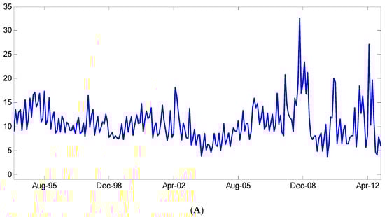
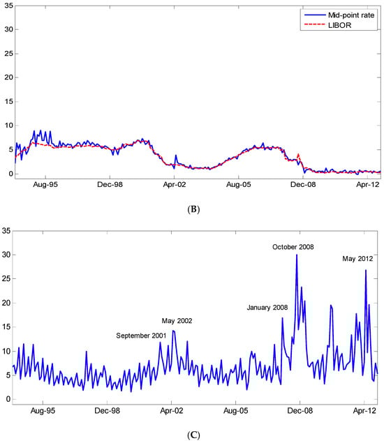
Figure 1.
Funding illiquidity measure. (We plot the time-series of the investor’s implied borrowing rate (A), the investor’s mid-point rate along with the LIBOR (B), and the difference between the implied borrowing rate and the mid-point rate—our funding illiquidity measure (C). All rates have a constant three-month maturity. The period is from January 1994 to December 2012.)
Next, we test if shocks to our funding illiquidity measure affect leveraged managed portfolios. We focus on hedge funds, which often use leverage in order to exploit arbitrage opportunities to enhance returns and provide liquidity (). Using a rolling windows approach, we sort hedge funds into decile portfolios according to their exposure to changes in funding illiquidity. We find that the portfolio with the most negative exposure to funding illiquidity, on average, earns higher returns than the portfolio with the most positive exposure to funding illiquidity. The spread is 39 basis points per month and significant with a t-statistic of 2.58. Thus, funds that are most exposed to shocks to funding illiquidity appear to earn a premium as compensation for the risk of low returns when funding liquidity deteriorates. We also show that the spread return is high and positive during normal times and negative during crisis periods when funding costs are high. Using recessions as identified by the NBER as a proxy for crisis periods, we find a spread of 56 basis points per month (t-statistic of 3.97) in normal times and −59 basis points during crisis periods (t-statistic of −3.46 for the difference with respect to normal times). This stark difference in returns between the normal and crisis periods provides further support that funding illiquidity is a source of risk. Importantly, the documented difference between normal and crisis periods is not driven by the survivorship bias or existing factors known to affect hedge fund returns, such as those used in () or ().
We also show that our measure contains new information for the cross-section of hedge fund returns. Specifically, our main results for normal and crisis periods are robust to using versions of our funding illiquidity measure that are orthogonal to default spread, term spread, the existing proxies for funding illiquidity (changes in TED spread or LIBOR–repo spread, changes in the treasury market arbitrage (), the leverage of broker–dealers factor (), changes in margin requirements (), the betting against beta factor (), and the tail measure ()) or market-wide illiquidity factors of (), (), and ().
The information content of our funding illiquidity measure is also distinct from the simple option bid–ask spread, the frequently used measure of option liquidity (). Indeed, our measure performs well when we adjust it for changes in either relative or absolute bid–ask spreads. Furthermore, our results strengthen when we adjust our funding illiquidity factor for changes in option market makers’ net demand. The latter result is intuitive because the underlying premise of our funding illiquidity measure is stable market makers’ net demand. Adjusting for changes in net demand therefore reduces any noise arising from fluctuations in demand imbalances. Our main results are also robust when we adjust for changes in VIX or changes in good and bad VIX (). This confirms that we are not merely picking up on times of uncertainty when delta-hedging by market makers may be more difficult.
Consistent with theory, our results suggest that the spread among the funding illiquidity-sorted portfolios is stronger for leveraged than unleveraged hedged funds. This result also extends to closed-end mutual funds, which generally use less leverage than hedge funds, but the data on leverage have better coverage, enabling a cleaner distinction between leveraged and unleveraged funds.
Finally, we analyze funding illiquidity risk in asset classes where leveraged investors are likely to be marginal investors. We look at carry trades, CDS–bond basis trades, and S&P 500 option portfolios. Using the () approach, we find a significant effect of funding illiquidity risk for high-yield CDS–bond basis trades and S&P 500 option portfolios and a weak effect for carry trades and investment-grade CDS–bond basis trades.
We foremost contribute to the literature on funding illiquidity. Like (), (), and (), we argue that funding illiquidity measures can be extracted from observable market prices. Differently from these studies, we focus on options markets, where the data on the positions of liquidity providers are readily available, and the directional effects of funding illiquidity are easier to determine. In comparison to the TED spread or the LIBOR–repo spread, our measure does not rely on the observable interest rates but rather on the rates implied in derivatives markets, which are subject to central clearing. As such, our measure is not prone to credit rationing or counter-party risk. Finally, our results suggest that funding conditions affect both leveraged investors as well as assets where leveraged investors are marginal investors. This is similar in spirit to (), who show that leverage of brokers–dealers helps explain cross-sections of many asset classes, or to (), who show that leverage constraints of active mutual funds help explain the cross-section of equity returns. Consistent with this literature, our results suggest that funding illiquidity shocks are an important source of risk. If some hedge funds have the ability to anticipate and manage such shocks, as argued by (), our results may actually understate the importance of funding illiquidity shocks.
We also contribute to the literature that emphasizes the role of demand and supply for option prices. () empirically show that option market makers’ net demand affects the option implied volatility surface. () develop a model where net demand for option market makers affects option prices. Instead, we argue that available capital is constrained, and funding illiquidity of the option market makers thus affects the implied borrowing rate in the market for S&P 500 derivatives. This is in line with ideas in three recent papers. () argues that option dealers use repo financing to hedge their inventory and shows how these funding costs may affect option quotes. () look at the net demand for deep out-of-the-money put options to analyze how options intermediaries manage tail risk. () link differences in the variance risk premium in the equity and options markets to the financial standing of intermediaries. Importantly, in our setting, controlling for net demand does not diminish but rather improves our results that funding illiquidity is an important driver of asset returns.
2. A Funding Illiquidity Measure Implied by S&P 500 Derivative Markets
Unlike equities, options are in zero net supply, with the market makers absorbing any excess demand from investors. For two reasons, this requires funding on the part of market makers.
First, market makers require capital to satisfy margin requirements. Market makers need to post margins for options as well as for trading the asset, which they use to hedge their options exposure.6 Because the basket of S&P 500 securities is expensive to trade and hard to short, market makers for S&P 500 index options typically hedge their exposure with S&P 500 futures. S&P 500 futures are very liquid, trade at tight bid–ask spreads, and are easily shorted but are subject to margin requirements. Thus, in the case of S&P 500 options, market makers require funding to post margins for both S&P 500 options and futures.
Second, market makers may not always be able to hedge perfectly due to indivisibilities, stochastic volatility, or the inability to hedge continuously (; ). Such difficulties in hedging require yet more funds to absorb the resulting risks and make funding illiquidity even more important. For both reasons, we expect market makers to quote option prices in line with their funding costs.
Conversely, option prices should reveal the funding conditions of option market makers. To the extent that individual market makers and market-making banks finance their activities through short-term collateralized financing (), namely through repos (),7 option prices should also be revealing more broadly about the market-wide funding shocks.
How exactly funding costs affect quoted option prices, however, depends on whether market makers have a net long or a net short position in options. In Table 1, we report demand imbalances in the market for S&P 500 options. We use OpenClose data from Market Data Express for the period from January 1994 to December 2012. Market makers’ net demand is defined as the negative of the aggregated non-market makers’ net demand (the sum of the net demands of firms, customers, and market makers needs to be zero). We distinguish between call and put options and sort options according to moneyness (strike price/index level) and time-to-maturity. What stands out most is the difference between the call and put options. Whereas market makers’ average net demand is typically large and negative for put options, it is smaller and positive for call options. This pattern is strongest for shorter maturity options and options with lower moneyness. With the increase in maturity and for the highest moneyness levels, demand imbalances weaken and may even flip signs.

Table 1.
Market makers’ net demand for S&P 500 options.
We thus concentrate on short-dated options with low moneyness, as here, demand imbalances are largest, and these options are therefore most sensitive to funding illiquidity. For this set of options, market makers are typically buying call options and selling put options. When funding deteriorates and hedging option exposure becomes more expensive, market makers want to pay less for buying call options (call bid decreases) and want to receive more for selling put options (put ask increases).
Holding everything else equal, for a pair of a call and a put with the same strike price ( and the same maturity , we expect an increase in funding costs to decrease the difference between the call bid price and the put ask price . By no arbitrage, the payoff from a long position in a call and a short position in a put is equivalent to the difference between the futures price and the strike price, .8 Therefore, to make the above difference comparable across options with different strike prices, we take the log of the ratio of both differences. To further make this ratio comparable across options with different maturities, we additionally divide it by the time-to-maturity:
We can distinguish between two cases where Equation (1) is well defined: case (i): and case (ii): . Case (i) involves mostly options with low moneyness, whereas case (ii) generally holds for options with high moneyness. Because market makers’ demand imbalances are larger for options with low moneyness (see Table 1) and options liquidity is skewed toward these options, we focus on the first case.
Also, for case (i), Equation (1) has an intuitive interpretation. In a world without margin requirements, it would provide us with an estimate of the implied borrowing rate from the perspective of a typical investor in the option market. In particular, ignoring margin requirements, an investor who sells a call option, buys a put option, and simultaneously buys the future initially receives the difference between the call bid and the put ask. At maturity, by no arbitrage, the investor needs to repay the difference between the futures price and the strike price. The log ratio between the cash flows therefore provides an estimate for the continuously compounded rate, which the investor would theoretically need to pay to borrow money in the derivatives market. Adjustment for the time-to-maturity (/) ensures that the borrowing rate is annualized. In reality, investors are subject to margin requirements. This makes borrowing in derivative markets difficult and expensive. Still, keeping this in mind, it is instructive to think of case (i) in Equation (1) as the implied borrowing rate.
As argued above, an increase in hedging costs due to an increase in funding illiquidity should decrease the difference between the call bid price and the put ask price. In turn, according to Equation (1), the implied borrowing rate increases. This leaves us with an intuitive prediction: the implied borrowing rate should reflect the funding conditions of option market makers in the market for S&P 500 derivatives.
Because the implied borrowing rate also captures the general level of interest rates, we subtract the mid-point rate from the implied borrowing rate. The mid-point rate is based on the options’ bid–ask mid-point and presents an average between the investor’s implied borrowing and the lending rates. In sum, we define our funding illiquidity measure as the difference between the implied borrowing rate and the mid-point rate:
where and similarly for the puts.
As we note below, subtracting LIBOR (rather than the mid-point rate) or simply relying on the implied borrowing rate without subtracting another rate affects our results only marginally.
2.1. Further Discussion of the Proposed Funding Illiquidity Measure
The estimation of the implied rates only requires market prices for options and futures. Because both are actively traded on the market, the proposed measure should capture market makers’ funding conditions in real time. Also, as guaranteed by options settlement procedures, our measure should be hardly affected by counter-party risk.
Furthermore, because S&P 500 option market makers hedge their positions using the highly liquid and easy-to-short S&P 500 futures rather than the basket of securities in the S&P 500 index, the potential effect of equity market illiquidity on our measure is limited. This is different for stock options, which are hedged with the underlying stock that is often illiquid and hard to short. In the empirical analysis, we show that our results are robust when we only use changes in our measure that are orthogonal to changes in market-wide liquidity measures.
In deriving our measure, however, we make the relatively strict assumption that demand imbalances for market makers are stable. In practice, option net demand varies over time. Examining the time-series variation in market maker’s net demand for shorter maturity, lower moneyness level options month by month, we note that the average net demand for call options is positive in 65% of the months and negative for put options in 82% of the months. The difference in the average net demand between calls and puts is positive in 80% of the months. Thus, the assumed positions do not always hold but are an accurate description for most of the months in our sample period. To further address the concern that changes in net demand, rather than changes in funding illiquidity, drive our results, we show that the difference in net demand for call and put options is only weakly related to our funding illiquidity measure. Also, our results even improve somewhat when we use only the funding illiquidity changes orthogonal to changes in net demand.
To the extent that market makers cannot always hedge perfectly, especially in times of high volatility (), our measure could pick up uncertainty and tail risk. To address this concern, we show that funding illiquidity is correlated with, but different from, VIX (as well as the downside VIX of () and the tail measure of ()). Also, our results are robust when we use only the funding illiquidity changes orthogonal to changes in the above measures.
Note that although our measure is based on the quoted prices, it is different from the simple options bid–ask spread. Unlike the bid–ask spread that is calculated for the same options, our measure combines bid and ask prices of different options and thus captures the asymmetric effects of funding illiquidity on bid prices for calls and ask prices for puts. Indeed, we show that our measure is correlated with the bid–ask spreads but still performs well when we adjust it for changes in either the relative or the absolute bid–ask spreads.
Finally, note again that we do not require that investors literally borrow in the derivative markets. We only conjecture that, through the mechanism explained above, our measure is correlated with the actual funding constraints of option market makers.
2.2. Data and Estimation
We use end-of-day prices for S&P 500 index options from Market Data Express and end-of-day prices for S&P 500 index futures from the Chicago Mercantile Exchange (CME). The time period is between January 1994 and December 2012, which matches the availability of our hedge funds data. We first eliminate options that violate the basic arbitrage relations. Next, to match expirations for options and futures, we keep only options that expire on a quarterly cycle.9
Based on Equation (1), we estimate the implied borrowing rate from put–call pairs where the bid price for a call is higher than the ask price for a put and the futures price is higher than the strike price. As discussed above, these are predominately options with moneyness levels below one. Because for at-the-money options, the put price is very close to the call price and thus, according to Equation (1), a small change in the option price can lead to rather large differences in the implied rates, we only use options with the moneyness level below 0.975. To further minimize microstructure noise, each end-of-month, we use the last 10 days of data and only options with open interest greater than 200 contracts. In untabulated results, we find that varying the moneyness level to below 0.96 or below 0.99 affects our results only marginally. Similarly, results are largely the same if we require options to have open interest larger than 150 or 250.
The above filters result in a total of 99,470 estimated rates in our sample period. The number of estimates increases over time and declines with maturity. We aggregate these estimates at the end of each month by taking the median across all rates with the same maturity. To obtain monthly rates with constant maturities, we interpolate linearly between yields with the closest maturities. We thereby obtain the term structure of implied borrowing rates with maturities between three and six months. In the main analysis, we base our funding illiquidity measure on the borrowing rates with the shortest, three-month maturity, as here, the demand imbalance for option market makers is the largest. In total, we have 228 monthly observations.
Using the same procedure and the same set of options, we also calculate the mid-point rate. The only difference between the borrowing rate and the mid-point rate is that we replace in Equation (1) the call bid with the call bid–ask mid-point and the put ask with the put bid–ask mid-point.
In addition, we define two different measures of the bid–ask spread. The first is the standard relative bid–ask spread, which is often used in studies on options illiquidity (). It is defined as the difference between the ask price and the bid price divided by the option mid-quote. We calculate the relative bid–ask spread from a wide set of options, using all options with open interest greater than 200 and maturity between 5 and 90 days. We only eliminate options with (mid-point) prices lower than USD 3 as these options have very large relative bid–ask spreads. The monthly time-series of relative bid–ask spreads is then the median across bid–ask spreads for call and put options over the last 10 days of data within a given month. Equation (1), however, suggests that our measure is closer to the absolute bid–ask spread than to the relative bid–ask spread. Also, in calculating our measure, we restrict ourselves to shorter maturity, lower moneyness level options. Therefore, as our second measure of bid–ask spread, we additionally construct the absolute bid–ask spread based on the same set of options that we use in calculating our funding illiquidity measure and using the same estimation procedure.
Finally, using OpenClose data, we calculate the monthly time-series of the difference between the market maker’s net demand for call and put options. During the last 10 trading days within each month, we use options with time-to-maturity between 5 and 90 days and a moneyness level below one. For each month, we first calculate average net demand separately across call and put options and then take the difference between those two averages.
2.3. Summary Statistics
In Figure 1, we present the construction of our funding illiquidity measure. Panel A plots the three-month implied borrowing rate, Panel B plots the corresponding mid-point rate, and Panel C plots the difference between the implied borrowing rate and the mid-point rate—our proxy for funding illiquidity. Three observations stand out. First, the implied borrowing rate is fairly high, around 10% on average. This is driven by the relatively high bid–ask spreads in the market for S&P 500 options. One of the reasons for such high bid–ask spreads is related to the fact that trading with S&P 500 options is limited to a single exchange, the Chicago Board of Options Exchange (). However, we are interested in the time-series variation of our measure, and the overall level of our measure is thus of little importance (in our main analysis, we use the first differences of our measure). Also, as much option trading occurs within the bid–ask spreads, our estimates can be seen as an upper bound on the implied borrowing rate. We repeat our study with a 50% reduced bid–ask spread; the rate decreases to 6%, while our main results remain virtually unchanged.
Second, the mid-point rate is very close to LIBOR and is substantially less volatile than the implied borrowing rate. As a result, most of the variation in our funding illiquidity measure comes from variations in the implied borrowing rate. As reported in Table 2, our funding illiquidity measure is 7.01% on average, has a standard deviation of 4.24%, and is relatively persistent with an autocorrelation coefficient of 0.53. Third, and most importantly, the funding illiquidity measure increases substantially during times of market distress. It reaches its maximum in October 2008 at 30.02%. This is a large spike on the order of five standard deviations away from the mean. Other large spikes appear in May 2012 at 26.77%, January 2009 at 23.31%, May 2002 at 14.25%, and September 2001 at 11.86%. These spikes can be associated with the stock market dropping precipitously in October of 2008 due to the financial crisis and the worries over the European debt crisis in May 2012. The June 2002 spike overlaps with a long downward move after the dot-com bubble, and the September 2001 spike coincides with the terrorist attacks of 9/11. Thus, our funding illiquidity measure appears to capture well times of market distress and illiquidity.
Table 2.
Summary statistics for the funding illiquidity measure and other variables.
In Figure 2, Panel A, we see that our funding illiquidity is correlated with futures margin requirements (correlation of 0.31 with absolute margins and 0.40 with relative margins). This works well with our intuition that market makers need more capital (and thus incur higher funding costs) if margin requirements are higher.
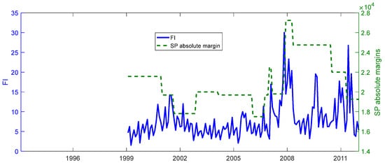
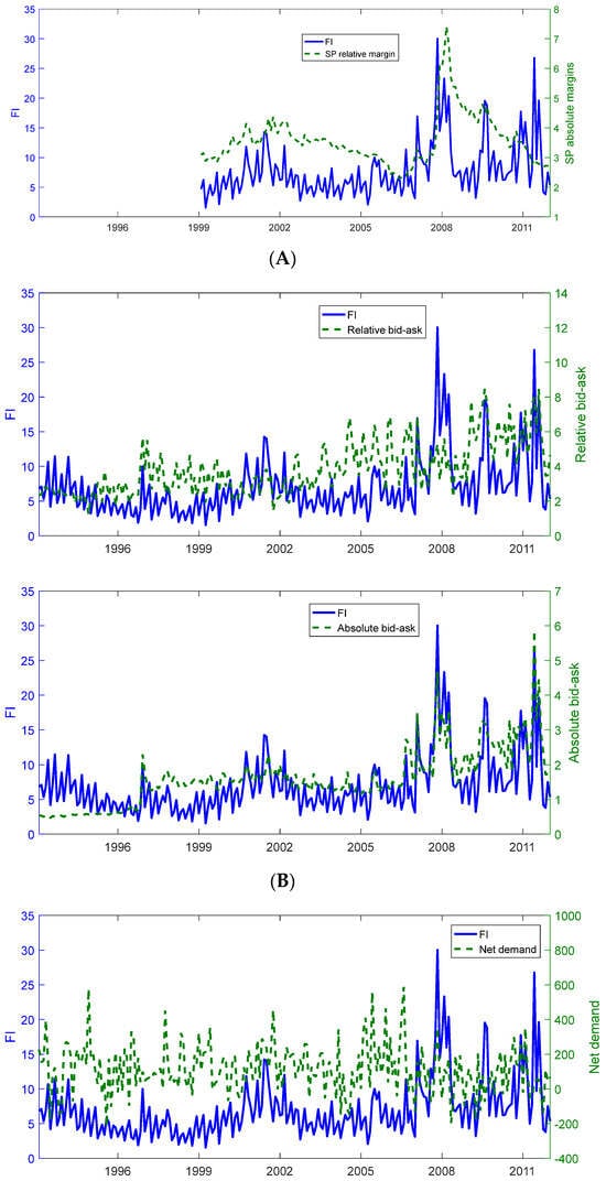
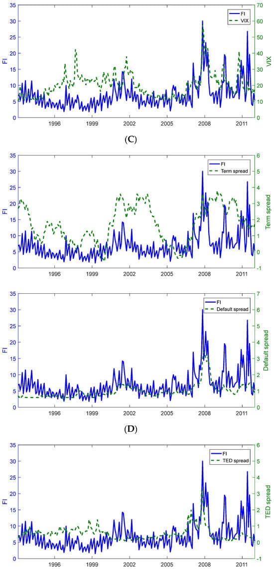
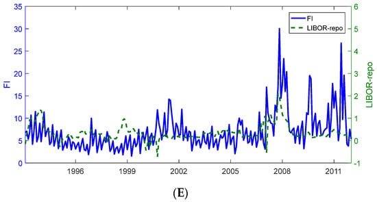
Figure 2.
Funding illiquidity versus alternative measures. (We plot the time-series plots of funding illiquidity along with the absolute or relative SP futures margin (A), relative or absolute bid–ask spread (B), funding illiquidity along with the net demand or VIX (C), funding illiquidity along with the term spread or default spread (D), and funding illiquidity along with the TED spread or LIBOR–repo spread (E). The period is from January 1994 to December 2012.)
To probe further, we next compare our funding illiquidity to (relative and absolute) bid–ask spreads, market maker’s net demand, and other measures of funding costs, credit conditions, and overall market uncertainty. The latter include the VIX index (S&P 500 options implied volatility index), the term spread, the default spread, the TED spread, and the LIBOR–repo spread. The data sources and variable definitions are provided in Appendix A.
In Figure 2, we plot each of the above variables against our funding illiquidity measure. The summary statistics are reported in Panel A of Table 2. As expected, our measure is strongly, but imperfectly, correlated with the option bid–ask spread measures. The pairwise correlation with the absolute bid–ask spread is 0.70, while the correlation with the relative bid–ask spread is lower at 0.43. The pairwise correlation with market makers’ net demand is close to zero at 0.04.
Importantly, our measure is positively related to all the variables related to credit conditions and market uncertainty. The pairwise correlations range between 0.20 for TED and 0.64 for default spread. It is also comforting to note in Figure 2 that the default spread exhibits spikes similar to those of our funding illiquidity measure. The time-series variation in other variables is more distinct. Overall, the evidence suggests that our measure captures times of market-wide worsening of credit conditions while adding independent variation.
In the main empirical tests, we use changes in our funding illiquidity measure (denoted the funding illiquidity factor, FI) rather than levels. Therefore, Panel B of Table 2 also reports the summary statistics for the first differences of all variables. The mean change in our funding illiquidity factor is effectively zero, with a standard deviation of 4.14%. The AR(1) coefficient for the differences is −0.40. This compares to −0.32 to −0.48 for changes in the bid–ask spread measures and net demand, −0.17 for the TED spread, and −0.21 for the LIBOR–repo spread. Once we take changes, the correlations between our funding illiquidity measure and the other variables are low, between −0.16 (for changes in LIBOR–repo spread) and 0.19 (for changes in net demand). The only exceptions are the relative and the absolute bid–ask spread, where the correlations remain approximately the same at 0.42 and 0.65, respectively.
- Other Funding Illiquidity Factors
Next, we compare our factor (changes in our funding illiquidity measure) to other funding illiquidity factors proposed in the literature. These include the treasury market arbitrage measure of (), the broker–dealer leverage factor of (), the () margin requirement measure, the “Betting against beta” factor for the U.S. equities of (), and tail measure of (). Details on data sources and the construction of variables are provided in Appendix A.
The summary statistics are reported in Panel A of Table 3. The first column specifies the time period for which we have the data on the alternative proxies for funding illiquidity. What stands out is that the pairwise correlations between the other funding illiquidity factors are fairly low. Also, our measure of funding illiquidity factor exhibits low correlations with the existing factors, between −0.05 and 0.19.
Table 3.
Summary statistics of the alternative funding illiquidity and market illiquidity factors.
- Market Illiquidity Factors
Finally, because funding illiquidity and market illiquidity may mutually reinforce each other in “liquidity spirals”, as shown theoretically by (), we additionally relate our funding illiquidity factor to market-wide illiquidity factors. We obtain the innovations in aggregate illiquidity of (), the transitory and permanent components for the () illiquidity factor, and the noise measure of ().10 The noise measure derives from no-arbitrage violations in the treasury market. As the noise variable is highly autocorrelated (0.92), we use differences. Again, details on data sources are provided in Appendix A.
The summary statistics are reported in Panel B of Table 3. All the illiquidity measures are available for the full period from January 1994 to December 2012. Again, we note that the correlations are relatively low. The pairwise correlations with our funding illiquidity factor range from −0.12 to 0.16. Also, all factors have low serial autocorrelations, between −0.13 and 0.11.
Finally, we explore to what extent our funding illiquidity measure predicts aggregate market returns and other funding or market liquidity measures one month into the future. As expected, we find that changes in our funding illiquidity measure are negatively related to future market returns (−0.24), and this correlation stems mainly from the crisis period. In a univariate regression, the t-statistic for predicting monthly returns is 1.84. We also find that changes in our measure predict many alternative factors. For funding illiquidity measures, it predicts treasury market arbitrage (t-statistic of 2.51 in a regression on lagged changes in funding illiquidity) and (changes in) margin requirements (3.21), while our regressions are insignificant for broker–dealer leverage and betting against beta. For market illiquidity measures, it predicts the permanent component of () (t-statistic of −1.73) and (changes in) noise (2.45), while we cannot predict the () liquidity measure and the transitory component of ().
3. Funding Illiquidity Risk and Delegated Portfolios
The previous section suggests that our funding illiquidity measure captures the general market conditions. Probing further, we next test whether shocks to our funding illiquidity measure are a source of risk for delegated portfolio management. Theoretically, funding illiquidity should affect only leveraged investors. The obvious candidates here are hedge funds because they often use high leverage to exploit arbitrage opportunities. We additionally analyze closed-end funds, which also use leverage, although to a smaller extent. In all our tests, we sort funds into portfolios based on their exposure to funding illiquidity risk.
As emphasized by (), a common issue in hedge fund studies is that the sample coverage is usually restricted by using a particular database. Moreover, different databases for hedge funds have little overlap in terms of coverage of hedge funds. In some cases, certain empirical regularities are prevalent in one database while not in other databases. As a result, these authors suggest that researchers deploy as many hedge fund databases as possible. A unique aspect of our data is that we combine together six hedge fund databases, which include Altvest (now part of Morningstar), BarclayHedge, CISDM Morningstar, HFR, Eureka, and TASS hedge fund databases, and create a comprehensive dataset. For details, see ().
We take care of the main biases contained in hedge fund databases in a way similar to (). Our merged database provides information on dead and alive funds, which decreases survivorship bias. To mitigate the backfilling bias, we delete the first 12 monthly observations. When estimating the MA(2) model of (), we find that around 70% of all hedge funds within our database exhibit significant smoothing coefficients. To adjust for the downward bias in the volatility of returns resulting from smoothing, we use the correction proposed by (). In our statistical tests, we require hedge funds to have at least 36 months of observations. After applying these data filters, there are 14,320 funds, with summary statistics presented in Table 4.
Table 4.
Hedge fund sample summary statistics.
Returns of a typical hedge fund from our sample are 51 basis points per month on average and are non-normally distributed with fat tails (average kurtosis in the sample 6.45) and negative skewness (−0.21). The average life span of a hedge fund is around 7 years. Among other characteristics we find in the database are the management fee (1.50% on average) and the performance fee (18.59% on average); 90% of hedge funds are open to new investments, and 82% use a high water mark. For a subset of funds that provide data on leverage, 48% are leveraged.
3.1. Hedge Fund Portfolios Formed by Funding Illiquidity Betas
To test the sensitivity of hedge fund returns to funding illiquidity, we proceed as follows. Let be the excess return in month t of hedge fund = 1, …, 14,320, and be the market excess return. We estimate the exposure of fund to the change in the funding illiquidity measure () by the following regression using 36 past returns:
where fund ’s exposure to the change in funding illiquidity is captured by the funding illiquidity beta, .
At the end of each month (February 1997 through December 2012), based on the regression model in Equation (3), we first estimate the pre-ranking for each fund using its previous 36 months excess returns between months and . As most hedge funds have more than 36 observations, we move a rolling window of 36 observations through each hedge fund return time-series. Then, we sort all hedge funds in-sample by their pre-ranking into decile portfolios. We obtain each fund’s return next month and compute equally weighted average returns for each of these decile portfolios. If any hedge fund is being delisted from the database, we put a zero instead of the missing return.11 We then compute the return spread between the portfolio consisting of funds with the most negative (portfolio 1) and the portfolio consisting of funds with the most positive (portfolio 10),
By repeating the previous two steps month by month, we obtain the whole time-series of hedge fund returns for each of the ten portfolios, as well as return spreads between the lowest and the highest -sorted portfolio. Post-ranking illiquidity betas are obtained by regressing the time-series of these portfolio returns on our funding illiquidity factor.
Recall that the funding illiquidity measure in the above regression is defined as , and Figure 1 clearly illustrates that the funding illiquidity measure increases during downturns of the economy. Thus, if funding illiquidity shocks are a source of risk, portfolio 1, consisting of hedge funds with the most negative exposure to the funding illiquidity measure, should earn higher returns on average as compensation for bearing funding illiquidity risk. By the same logic, portfolio 10, consisting of hedge funds with the most positive exposure to the funding illiquidity measure, should earn lower returns. In other words, the spread between portfolio 1 and portfolio 10 returns should be positive.
Table 5 reports the basic characteristics of the portfolios sorted by funding illiquidity beta. The first three columns report the funding illiquidity betas during the portfolio formation period, the funding illiquidity betas in the months after portfolio formation, and the returns associated with funding illiquidity beta-sorted portfolios. Portfolio 1 has a pre-ranking beta of −0.65, whereas portfolio 10 has a pre-ranking beta of 0.38. By construction, the difference between portfolio 1 and 10 is negative at −1.03 and highly significant. Importantly, the post-ranking illiquidity beta difference between portfolios 1 and 10 remains negative, although it is more modest, as expected. It amounts to −0.11 with a t-statistic of −1.77. To adjust for the overlap induced by the rolling window approach, we use () t-statistics with 35 lags. Turning to the portfolios’ excess returns, portfolios with more negative exposure to funding illiquidity earn higher returns than portfolios with less negative exposure to funding illiquidity. The relationship is monotonic for the first six portfolios with the most negative exposure to funding illiquidity and then flattens out for the remaining four portfolios. The correlation between the portfolios’ pre-ranking betas (post-ranking betas) and portfolios’ average returns is negative at −0.82 (−0.96). In terms of the magnitudes, portfolio 1 earns 83 basis points on average in excess returns per month (t-statistic of 3.11), whereas portfolio 10, on average, earns 44 basis points in excess returns per month (t-statistic of 2.68). The return spread between portfolio 1 and portfolio 10 is positive at 39 basis points and statistically significant with a t-statistic of 2.58. This suggests that exposure to our funding illiquidity factor impacts hedge fund returns in the cross-section, as predicted by the theory.
Table 5.
Returns from funding illiquidity beta-sorted hedge fund portfolios.
In the last columns of Table 5, we also report some differences in hedge fund characteristics across funding illiquidity beta-sorted portfolios. Most differences are economically small and do not necessarily line up with the returns. For example, there is no difference between low versus high funding illiquidity beta-sorted portfolios’ management fees, performance fees, and proportion of funds that use high watermarks. We only observe a significant difference with respect to the openness to new investors, where funds with the most negative exposure to funding illiquidity shocks are less likely to accept inflows, although the difference is economically small.
For the full sample period, we also do not observe any statistically significant difference in the percent of delisted hedge funds among different decile portfolios. Examining delistings month by month, we do find, however, more delistings during the global financial crisis, especially for hedge funds most sensitive to funding illiquidity, aligned with funding illiquidity being a source of risk. For example, in December 2008, delistings among the hedge funds with the largest exposure to funding illiquidity risk are 16.9%, in comparison to 10.8% for hedge funds with the smallest funding illiquidity exposure.
Our sample period covers at least two crisis periods, namely the recessions identified by the NBER: March through November 2001 and December 2007 through June 2009. If funds can anticipate large funding illiquidity shocks, we should observe no difference in the hedge fund portfolio spreads between the normal and crisis periods. However, if funding illiquidity shocks are a source of risk, as conjectured above, then funds that are most exposed to funding illiquidity risk should earn a positive return in normal times but would be hit with a negative return in times of funding illiquidity if they need to shed assets at fire sale prices.12 Consistent with the risk-based explanation, we indeed find that the average hedge fund return spread is positive at 56 basis points per month in non-crisis periods and negative at −59 basis points per month during the crisis periods. We formally test for the difference below. To illustrate the effect, we plot in Figure 3 the twelve-month moving average of the hedge fund return spread between portfolio 1 and portfolio 10, along with the NBER recessions. The plot confirms that the spread is positive during non-crisis periods, especially during the dot-com bubble and in the aftermath of the global financial crisis. At the same time, it is negative during both crisis periods, and the dip is largest during the last and the most severe recession. The only observation not covered by the NBER recessions is the negative spread in 2012, which may be related to the fear of a European debt crisis (referring to Figure 1; note that this period also coincides with a rather high funding illiquidity measure). We will thus account in our analysis for both normal and crisis periods.
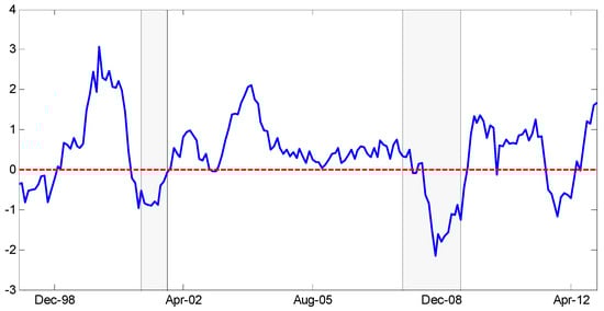
Figure 3.
Hedge fund return spread. (We plot the time-series of the spread return between the hedge funds portfolio 1 and portfolio 10 along with the NBER recession periods (in gray). The figure is based on the twelve-month moving average return of the hedge fund return spread. The return spread is expressed in percentages.)
3.2. The Four Models of Sorted Portfolio Returns
To formally examine the return spreads between the lowest and the highest -sorted portfolios, we run four tests. First, we run a standard t-test on returns, which is equivalent to the estimation of the following model (Model Constant):
where is the intercept term for the full sample.
Next, we examine returns of illiquidity beta-sorted portfolios during normal and crisis periods. We investigate this by estimating the following regression model (Model Crisis):
where is the intercept term for the full sample, and is a dummy variable that takes the value one during crisis periods and zero otherwise. Thus, the non-crisis period alpha of the funding illiquidity beta-sorted portfolios is , and the crisis period alpha of the funding illiquidity beta-sorted portfolios is .
Finally, we consider two benchmark factor models. The first one is the traditional () seven-factor model that includes two equity-oriented factors, three trend-following factors, and two bond-oriented factors downloaded from David Hsieh’s Hedge Fund Data Library.13 The second benchmark model is a ten-factor model recently developed by (; NPPR hereafter). NPPR extracts the first 10 return-based principal components (PCs) from 251 global assets across different countries and asset classes and shows that these 10 PCs explain, on average, some 99% of the variability in the returns of the considered assets.14 The exact specification of our regression model is as follows:
where factors are either the seven () factors (Model FH) or the ten NPPR factors (Model NPPR). All t-statistics are based on (), with 35 lags. Using the optimal lag length according to (), all our main results remain strongly significant.
3.3. The Baseline Result
Column (1) of Table 6 presents our baseline result. As noted above, in the full sample period, hedge funds with the most negative exposure to funding illiquidity outperform funds with the most positive exposure to funding illiquidity by 39 basis points per month (t-statistic of 2.58). During normal periods, the funding illiquidity spread is positive at 56 basis points per month and highly significant (t-statistic of 3.97). In contrast, during crisis periods, the funding illiquidity spread is negative at −59 basis points per month. The difference between the two spreads is 1.15% per month and highly significant with a t-statistic of −3.46. This stark difference in returns between the normal and crisis periods provides further support that funding shocks are a source of risk for the hedge fund industry. Using the () seven-factor model as the benchmark model, we find that the spread is only partially driven by the existing hedge fund pricing factors. During normal periods, the spread is 43 basis points per month (t-statistic of 3.64), whereas it is negative at −45 basis points per month during the crisis periods when funding illiquidity is high (the difference is significant with a t-statistic of −3.09). A similar picture emerges for the NPPR model. During normal periods, the spread is also 43 basis points per month (t-statistic of 2.57), while it is negative at −68 basis points per month during times of high funding illiquidity (t-statistic for the difference of −4.26).
Table 6.
Returns from funding illiquidity beta-sorted hedge fund portfolios, main tests.
Because of the voluntary nature of hedge fund reporting, a delisting may not reflect the death of a fund but rather a failure to report after a string of bad performances, which could bias our results. To address this concern, we show in column (2) of Table 6 that the results remain largely unchanged if we set delisting returns to minus 10% rather than zero.
- Does Our Funding Illiquidity Measure Provide New Information for the Cross-section of Hedge Fund Returns?
In this section, we ask whether our funding illiquidity measure provides information for the cross-section and time-series of hedge fund returns beyond bid–ask spreads, other option implied variables, alternative proxies for funding illiquidity, and measures of market illiquidity. To test this, we repeat our hedge funds’ tests on a funding illiquidity measure that is orthogonal to these variables. We first regress our funding illiquidity factor (changes in funding illiquidity) on changes in a particular variable (factor). We then use the residuals from this regression and repeat all four tests of portfolio-sorted hedge funds. We use one variable at a time.
- Bid–ask spreads, Net demand, and VIX
Our time-series analysis suggests that changes in funding illiquidity are most closely related to changes in the options’ relative and absolute bid–ask spreads, with pairwise correlations of 0.42 and 0.65 (Table 2, Panel B). Therefore, we first orthogonalize our funding illiquidity factor with respect to changes in those two variables. Results are reported in Table 6, columns (3) and (4). For the full sample, the hedge fund return spread hardly moves to 39 and 37 basis points per month, although the t-statistic of the constant decreases from 2.58 to 1.67 and 1.65, respectively. For the normal versus crisis periods, all the results remain economically and statistically strong. When we control for the factors known to affect hedge fund returns, the estimates even increase and become more significant. Thus, our funding illiquidity measure captures information that goes beyond the simple option bid–ask spread. In untabulated results, we note that we cannot replicate our results using either the relative or absolute option bid–ask spread, as the resulting hedge fund return spread is small and insignificant in all our models.
We continue the analysis using a funding illiquidity factor that is orthogonal to changes in net demand. As we can see in Table 6, column (5), our results strengthen. In the full sample, the hedge fund return spread increases from 39 to 49 basis points per month, and the corresponding t-statistic increases from 2.58 to 3.58. Also, all the results for the normal times versus crisis periods are overall stronger. This improvement is aligned with our intuition. Recall that we derive the funding illiquidity measure under the assumption of stable market makers’ net demand. Any variation in net demand therefore introduces noise in our funding illiquidity measure. Removing the common variation in both variables should then improve the measurement of funding illiquidity.
Next, we use implied measures of uncertainty. In Table 6, column (6), we report results for the funding illiquidity factor that is orthogonal to changes in VIX. All our results for the normal times and the crisis periods are very comparable to the baseline case. The t-statistic only decreases in the full sample somewhat to 1.94.
As volatility risk could be asymmetric, we also use the data from (), who separate good and bad VIX depending on the in-the-money and out-of-the-money options. Our results in Table 6, column (7), strengthen, and the Crisis Dummy t-statistic increases by more than one. All in all, we conclude that our funding illiquidity measure contains information that is largely orthogonal to the analyzed option implied variables.
- Term Spread and Default Spread
Next, we orthogonalize our funding illiquidity measure with respect to changes in the term spread and the default spread. Results are reported in Table 6, columns (8) and (9). For the term spread, the results are very comparable to the baseline case. For the default spread, results remain statistically strong, and the economic magnitudes of the documented effect increase somewhat. In the full sample, the spread increases from 39 basis points per month to 47 basis points per month.
- TED Spread and LIBOR–repo Spread
In the remaining two columns of Table 6, columns (10) and (11), we use funding illiquidity factors that are orthogonal to either changes in the TED or the LIBOR–repo spread. In the full period, our results weaken slightly. This is expected because, just like the TED and the LIBOR–repo, our measure is effectively a spread between two interest rates. The decrease in results, however, is rather small. In the full sample, the hedge fund return spread decreases from 39 to either 33 or 28 basis points per month and remains significant at either a five or ten percent level (t-statistic of either 2.14 or 1.71). Also, all the results for normal versus crisis periods remain strong and very comparable to the baseline case. This suggests that our funding illiquidity measure also captures information for the cross-section of hedge fund returns beyond the frequently used interest-rate-based funding illiquidity proxies.
- Alternative Funding Illiquidity Factors
Next, we use versions of our funding illiquidity factor that are orthogonal to either of the alternative funding illiquidity factors proposed in the literature, such as changes in the treasury market arbitrage measure from (), the leverage of broker–dealers from (), changes in the margin requirements from (), the betting against beta factor of (), and the tail measure of (). Results are reported in Table 7, columns (1) through (5). Although alternative proxies for funding illiquidity are not always available for the full sample period (see Table 3 for details) and broker–dealers leverage is available only at the quarterly frequency (we assume no within-quarter variation), the main takeaways are very comparable. Two observations stand out. The statistical significance of the hedge fund spread in the full sample decreases slightly but remains significant with t-statistics of around two. For normal versus crisis periods, all results remain strong and significant. Overall, although there might be some overlap in the information between different variables, our funding illiquidity measure provides information about the cross-section of hedge fund returns that is largely orthogonal to the alternatives proposed in the literature.
Table 7.
Returns from funding illiquidity beta-sorted hedge fund portfolios, additional tests.
- Market Illiquidity Factors
Finally, funding illiquidity is related to market illiquidity, and both may mutually reinforce each other in times of distress (). Therefore, we next repeat our analysis with funding illiquidity measures that are orthogonal to other frequently used measures of market illiquidity, such as the () liquidity measure, the transitory and permanent components of liquidity from (), and changes in the noise measure of ().
Results are reported in columns (6) through (9) of Table 7. All our main results from column (1) of Table 6 remain largely unchanged. The only exception is the full-sample hedge funds return spread in the case of the noise measure, where the spread drops by half and becomes insignificant. However, even in the case of noise, all our results for normal versus crisis periods remain strong and significant. This indicates that our funding illiquidity measure is also different from the existing market-wide illiquidity measures.
3.4. Funding Illiquidity and Leverage
Theoretically, the importance of funding illiquidity increases with the investors’ leverage. Unfortunately, data on hedge fund leverage are often incomplete. In particular, the definition of leverage varies across databases, and the information on leverage is often missing.15 Using the available data, we identify 3580 hedge funds as leveraged and 3403 as unleveraged (for 7337 funds, the information on leverage is missing). We then form funding illiquidity-sensitive portfolios and calculate the average spread for extreme portfolios, separately for leveraged and unleveraged hedge funds. In untabulated results, we find that the spread for leveraged hedge funds is 44 basis points per month and significant (t-statistic of 2.59), and the spread for unleveraged hedge funds is 29 basis points and insignificant (t-statistic of 1.57). Thus, although there are many missing observations for hedge fund leverage, we do find suggestive evidence consistent with funding illiquidity being more important for leveraged hedge funds.
Hedge funds, however, are not the only leveraged investors. () argue that leverage also plays an important role for closed-end mutual funds. For closed-end funds, we have more reliable data on the use of leverage and can better separate leveraged from unleveraged closed-end funds.
We obtain data on closed-end funds and their use of leverage from the Morningstar mutual fund database. Table 8 reports the summary statistics. There are, in total, 2206 closed-end funds in our sample in the period between January 1994 and December 2012, 31% of which use leverage. The monthly average return is 30 basis points per month and comes with a 5.77% standard deviation. The funds are, on average, 8.5 years old and charge 82 basis points in management fees.
Table 8.
Closed-end fund sample summary statistics.
As in the hedge fund analysis, we form funding illiquidity-sensitive portfolios and calculate the average spread for extreme portfolios, separately for leveraged and unleveraged closed-end funds. Results are reported in Table 9.
Table 9.
Returns from funding illiquidity beta-sorted leveraged and unleveraged closed-end fund portfolios.
For leveraged closed-end funds, the basic empirical regularities from hedge funds carry over. The difference in post-ranking betas between the portfolio with the most negative exposure to the funding illiquidity risk (portfolio 1) and the portfolio with the most positive exposure to the funding illiquidity risk (portfolio 10) is as expected negative at −0.30 and significant (t-statistic of −6.73). Moreover, portfolio 1 earns, on average, 86 basis points per month (t-statistic of 2.31), whereas portfolio 10 earns, on average, 39 basis points per month (t-statistic of 0.95). Thus, the full-sample average return spread between portfolio 1 and portfolio 10 is 47 basis points per month and significant with a t-statistic of 2.56.
In comparison, for unleveraged funds, the difference between post-ranking betas between portfolio 1 and portfolio 10 is much smaller at −0.17, although still significant (t-statistic of −2.49). The spread between returns for portfolio 1 and portfolio 10, however, is negative at −25 basis points per month and insignificant with the t-statistic of −0.90.
We also find that the return spread for unleveraged funds is significantly different from the return spread for leveraged funds, with a t-statistic of 1.77. Thus, as suggested by theory, funding illiquidity risk affects leveraged more than unleveraged closed-end funds.
4. Funding Illiquidity and Returns from Other Asset Classes
Funding illiquidity may affect not only the portfolio returns of leveraged investors (e.g., hedge funds) but also the underlying asset prices, especially of securities where leveraged investors are likely to be marginal investors. For example, (), (), (), and () attribute part of the negative CDS–bond spread during the recent financial crisis to increased funding illiquidity. () show that unwinding of carry trades by speculators due to funding illiquidity shocks may lead to sudden changes in exchange rates unrelated to fundamentals.
As an additional test asset, we include S&P 500 option portfolio returns. In Section 2, we argue that funding illiquidity affects the hedging costs of option market makers, which in turn influences option prices. As market makers’ demand imbalances differ across option strike prices and time-to-maturity, different options would be affected by funding illiquidity differently. Also, market makers cannot hedge their option exposure perfectly due to stochastic volatility and the impossibility of hedging continuously (). Again, restrictions on hedging depend on option characteristics, with out-of-the-money options being the most difficult to hedge. For this reason, we now explore how funding illiquidity affects the returns of different option portfolios.
We recognize a type of circularity stemming from the fact that our measure of funding illiquidity itself is derived from option prices. Yet, as funding illiquidity derives from option prices while we analyze returns in relation to changes in funding illiquidity, we still feel that it is a worthwhile investigation.
4.1. Data for Carry Trade Portfolios, CDS–Bond Basis, and S&P Option Portfolios
We obtain the monthly data for the credit default swap CDS–bond basis primarily from Datastream. When the pricing information is not available from Datastream, we use the data from Bloomberg. The time period is from July 2002 to March 2010. We winsorize the data at 10% to mitigate the effect of outliers. Based on credit ratings, we distinguish between investment-grade and high-yield bonds.
For carry trade portfolios, we use the combination of two datasets: 6 portfolios from ()16 and 6 portfolios from ()17 sorted based on their interest rates (similarly to ). As the underlying data sources for the two sets of portfolios differ, the 12 portfolios are not perfectly correlated. We use monthly returns between February 1994 and January 2010.
Additionally, we use monthly returns on 54 portfolios of S&P 500 European-style options between February 1994 and January 2012 from (). These are portfolios of either calls or puts targeting the following moneyness ratios: 0.90, 0.925, 0.95, 0.975, 1.00, 1.025, 1.05, 1.075, or 1.10; and one of the three maturities: 30, 60, or 90 days. The portfolios are weighted averages of options with characteristics close to the moneyness and maturity targets. After a one-day holding period, the portfolios are being rebalanced to target. Returns are aggregated to the monthly level and scaled such that they have a target market beta of one.18
Table 10 reports the summary statistics. The CDS–bond basis is negative on average; minus 55 basis points per month for investment-grade bonds and minus 27 per month for high-yield bonds. The average returns for carry trades and option portfolios are positive on average: 19 basis points per month for carry trades and 25 basis points per month for options.
Table 10.
Summary statistics for different asset classes.
4.2. Empirical Models and Results
To test the impact of funding illiquidity risk on the portfolios of different asset classes, we now depart from the previous methodology and rely on Fama–MacBeth regressions. This choice is driven by the rather limited number of portfolios for some of the asset classes (e.g., there are only 12 carry trade portfolios and 54 option portfolios) and the short time-series of the individual CDS–bond basis, rendering the rolling window and sorting approach infeasible. We thus proceed as follows. In the first-stage time-series regression, we regress the asset’s return (or CDS–bond basis) in excess of the risk-free rate on the market excess return and the funding illiquidity factor:
In the second-stage cross-sectional regression, we regress asset returns (or CDS–bond basis) on the estimated risk loadings, separately for each month t:
where and are the beta estimates from the first-stage time-series regression. Finally, we obtain the time-series averages of the risk premiums on the market and on funding illiquidity, and . () voice concerns that model misspecification, as well as estimation errors in the betas from the first-pass time-series regressions, might affect the standard errors of . We therefore add an errors-in-variables adjustment term and a misspecification adjustment term to correct the standard errors.
Results are reported in Table 11. In column (1), we first check for the factor risk premiums for our funding illiquidity measure and the market in hedge fund returns. We use the 10 funding illiquidity-sorted hedge fund portfolios described above and assume that all funds within a given portfolio have the same post-ranking betas (). We note that the funding illiquidity, as captured by our measure, is indeed priced among hedge funds. The associated risk premium is −3.40% per month and is significant with the t-statistic of −2.36.19 The negative funding illiquidity risk premium is aligned with our previous results. Funding illiquidity increases in down markets. Funds with positive exposure to funding illiquidity therefore serve as a hedge against market downturns and command a negative risk premium. The market risk premium among the funding illiquidity-sorted portfolios is low and insignificant.20
Table 11.
Fama–MacBeth regressions of funding illiquidity and asset class returns.
Among the other asset classes21, we first present results for the CDS–bond basis. In particular, during the global financial crisis, when funding costs increased, we often observed a substantially negative CDS–bond basis. The more negative the funding illiquidity exposure is for an arbitrageur, the higher compensation the arbitrageur requires to engage in the trade (). Aligned with this intuition, we find that the average CDS–bond basis is negatively related to its exposure to our funding illiquidity factor. The relationship is weak for investment-grade CDS–bond basis (correlation of −0.28) and stronger for high-yield CDS–bond basis (correlation of −0.55). Accordingly, we find in Table 11, columns (2) and (3) that the funding illiquidity risk premium is negative and stronger for high-yield bonds. In the full sample, the premium is −7.48% per month and insignificant, whereas it is −11.20% and marginally significant for the high-yield bond with the t-statistic of −1.67. Splitting the sample, we find that the funding illiquidity risk premium is small and insignificant during normal times and high and significant during crisis periods for both investment-grade and high-yield CDS–bond bases. For the market excess return as a control variable, the risk premium is negative and significant for investment-grade bonds and insignificant for high-yield bonds.
Next, we analyze the carry trade portfolios, where we combine two data sets and use a total of 12 portfolios to improve the power of our tests. Carry trade returns decrease monotonically from portfolio 1 (high-interest-rate currencies) to portfolio 12 (low-interest-rate currencies). This is what gives rise to the popular carry trade. In the first stage (Equation (8)), we find that portfolio 1 has a lower funding illiquidity beta than portfolio 12, and the relation between the portfolio excess returns and funding illiquidity betas is close to monotonic (correlation of −0.68). This suggests that the higher excess returns for portfolio 1 are related to higher exposure to funding illiquidity risk. Our results in Table 11, column (4) suggest that the funding illiquidity risk premium is indeed negative at −7.79% per month, but it turns out to be marginally insignificant with a t-statistic of −1.31, possibly due to low statistical power as we only have 12 observations in the second stage of Fama–MacBeth. Probing further, we use the factor risk premiums estimated from hedge fund returns to calculate the two-factor (market plus funding illiquidity) alpha for all 12 carry trade portfolios, as in (). We find that the resulting alphas are almost all insignificant. We conclude that, although we do not find significant evidence for funding illiquidity being priced in the cross-section of carry trade portfolios, funding costs nevertheless seem to matter for the exploitation of the return differential between the high and low-interest-rate currencies.
Finally, we analyze option portfolio returns. Returns on put option portfolios tend to be higher than returns on call option portfolios. Furthermore, among the put option portfolios, especially those with shorter maturity and low moneyness, put options have the highest returns. Because market makers’ demand imbalances are most pronounced for the put options and delta-hedging is more difficult for out-of-the-money options, these are the option portfolios that would be most prone to funding illiquidity risk. Indeed, in the first stage (Equation (8)), we find that these portfolios have the most negative exposure to funding illiquidity. Overall, the correlation between the exposure to funding illiquidity and portfolio excess returns is very strong at −0.97. In line with this observation, we find in Table 11, column (5), that the funding illiquidity risk premium for options portfolios is negative at −8.35% per month and significant with a t-statistic of −2.69. In comparison, the market risk premium is 0.50% per month, but insignificant. Repeating the analysis separately for call and put options, we confirm that the results are mainly driven by put options. We find a strong and significant funding illiquidity risk premium for put options and an insignificant premium for call options.
Overall, our analysis suggests that our funding illiquidity factor affects not only the returns of leveraged managed portfolios (e.g., hedge funds) but also matters for assets where leveraged investors are likely to be the marginal investors.
5. Robustness Analysis and Additional Tests
In this section, we analyze the sensitivity of our results to changes in methodology and the measurement of funding illiquidity. All robustness checks are reported in Table 12 and refer to our main results reported in column (1) of Table 6, which we duplicate for convenience in column (1) of Table 12.
Table 12.
Returns from funding illiquidity beta-sorted hedge fund portfolios, robustness, and additional tests.
Our first robustness check entails the estimation of all regressions over 48 months instead of 36 months. As we show in column (2), all point estimates stay close to the main results and even increase slightly. Trying samples below 36 months weakens the results due to the larger standard errors caused by the shorter regression samples.
Next, we allow the factor loadings to vary over the business cycle by interacting factors with the Crisis Dummy. Results are reported in column (3) and are comparable to the results in the main analysis, where we impose constant factor loadings. In the main analysis, we define our funding illiquidity measure as the implied borrowing rate minus the mid-point rate. Instead, we now redefine funding illiquidity as simply the implied borrowing rate by itself (column 4), as the implied borrowing rate minus LIBOR (column 5), or as the implied borrowing rate minus the T-bill rate (column 6). All measures are based on the 3-month rates. Results are comparable to the main analysis. This is reassuring and also confirms that the main driver for our results is the investor’s borrowing rate rather than the mid-point rate.
We are also concerned about seasonality in our funding illiquidity measure, which could be introduced by the linear interpolation of implied borrowing rates that are tied to the quarterly cycle of futures expirations. A potential warning sign to us is the serial correlation of our funding illiquidity factor of −0.40 in Table 3, Panel A. We thus deseasonalize the time-series of funding illiquidity factor. Instead of making changes in the funding illiquidity measure, we subtract the moving average of the previous 3 months from the funding illiquidity measure. This reduces the serial correlation to 0.1. Repeating our main tests, we find that the results in column (7) of Table 12 are similar to our main findings but for a somewhat higher spread in the full sample and weakening of the crisis dummies.
Finally, we exclude the dot-com boom of the late 1990s and re-run our regressions for the period January 2000 through December 2012. The results are reported in column (8) and are qualitatively similar to the full-sample results.
6. Conclusions
We suggest a novel funding illiquidity measure that focuses on the role of market makers in the market for S&P 500 options. Based on market makers’ funding requirements and their typical positions, we extract our measure from quotes of S&P 500 options. Intuitively, our measure is closely linked to the investors’ implied borrowing rates. It captures well times of illiquidity and is correlated with several proxies for credit conditions and market uncertainty. It favorably competes with the alternative measures of (), (), and (). For a model of funding illiquidity, see ().
Funding illiquidity should especially affect leveraged managed portfolios, and we show that it explains cross-sectional variation in hedge fund returns (see ()). Hedge funds with negative exposure to changes in funding illiquidity earn high returns in normal times and low returns in crisis periods when funding liquidity deteriorates. Controlling for the existing hedge fund factors does not much affect our results. Importantly, the results are not driven by commonality with the established funding or market illiquidity proxies, as our results survive even when we only use the part of our measure that is orthogonal to each alternative measure.
Extending the analysis to closed-end mutual funds, we find that funding illiquidity matters for leveraged but not for unleveraged funds. Furthermore, we investigate asset classes where leveraged investors are marginal investors, as funding illiquidity might also affect their returns. Indeed, option portfolios with different option characteristics are exposed to funding illiquidity risk, with most of the exposure being related to the put options. CDS–bond basis trades for high-yield bonds are marginally exposed to funding illiquidity risk, while exposures for CDS–bond basis trades for investment-grade bonds and for carry trade portfolios are insignificant. Collectively, the evidence suggests that funding illiquidity is an important source of risk.
A further refinement that may sharpen the accuracy of our illiquidity measure is to incorporate insights from the stochastic dominance literature. These insights allow the distinction between the equilibrium values of options in a world without and with friction. This literature is still evolving, but the results of (), (), and () allow us to distinguish the cases where it is not possible to extract that measure from option values within the bid–ask spread. This is certainly a direction that should be the focus of future research.
Last, extending the funding illiquidity measure to other markets or asset classes would involve adapting the methodology to account for differences in market structure, liquidity, and the availability of data on market maker positions. We leave these ideas to future work.
Author Contributions
All authors equitably shared in developing the conceptualization, methodology, software, validation, formal analysis, data curation, writing, and visualization. All authors have read and agreed to the published version of the manuscript.
Funding
This research received no external funding.
Data Availability Statement
Data are contained within the article.
Conflicts of Interest
Author Anna Slavutskaya is employed by the company Finyon Consulting AG. The remaining authors declare that the research was conducted in the absence of any commercial or financial relationships that could be construed as a potential conflict of interest. The Finyon Consulting AG had no role in the design of the study; in the collection, analyses, or interpretation of data; in the writing of the manuscript, or in the decision to publish the results.
Appendix A. Additional Data Sources
This appendix details the data sources and variable definitions for all the variables used in Section 2. Unless specified otherwise, the variable is available on a monthly basis for the whole time period, January 1994 through December 2012.
We obtain the VIX index from the Chicago Board of Options Exchange (CBOE). The main interest rate variables are from the Federal Reserve Bank of St. Louis (FRED, H.15). The only exception is the repo rate, which we obtain from Datastream. The repo rate also starts only in October 1999. As it is highly correlated with the discount window borrowing rate from the H.15 reports (correlation above 0.9), we first regress the repo rate on the discount rate from October 1999 to December 2002. Based on that regression, we then reconstruct the earlier repo rate back to January 1994. We define all the interest rate-related variables in the standard way; TED spread is 3-month LIBOR over 3-month T-bill, LIBOR–repo spread is the spread between 3-month LIBOR and the repo rate, default spread is the spread between BAA- and AAA-rated corporate bonds, term spread is the spread between the yield on 10-year treasury bonds and the 3-month T-bill rate.
Other measures for funding illiquidity come mainly from authors’ webpages. In particular, we obtain the monthly treasury market arbitrage measure of () from January 1994 to March 2012 from Jean-Sebastien Fontaine’s webpage.22 The “Betting against beta” factor for the U.S. equities of () is from AQR’s webpage.23 We obtain the broker–dealer leverage factor of () from January 1994 to December 2009 from Tyler Muir’s webpage.24 We reconstruct the tail measure of () using OpenClose data from Market Data Express. Because the data on the broker–dealer leverage factor are quarterly, we define monthly observations by the last available quarterly observation.25 Finally, we reconstruct the () margin requirement measure using their method and margin data starting in January 2000, which we downloaded from the Chicago Mercantile Exchange (CME).26 Because the margin and treasury market arbitrage data demonstrate a high AR(1) of 0.90 and 0.93, respectively, we use first differences instead of levels in our analysis.
The market-wide illiquidity measures also come from the author’s webpages. In particular, we obtain the monthly innovations in the aggregate illiquidity of () from Lubos Pastor’s webpage.27 We download the monthly transitory and permanent components for the () illiquidity factor from Ronnie Sadka’s webpage.28 Finally, we obtain the monthly noise measure of () from Jun Pan’s webpage.29 All the market illiquidity measures are available for the full period from January 1994 to December 2012.
Notes
| 1 | () model the interaction between funding illiquidity and market illiquidity. () show the effects of capital-constrained financial intermediaries. Other recent theoretical contributions on the effects of limits to arbitrage, slow-moving capital, and the effect of margining include (), (), (), (), and (). |
| 2 | FINRA rule 4110 (SEA Rule 15c3-1) limits the aggregate indebtedness-to-equity ratio for market makers at 15 (8 during the first 12 months of operation) or, alternatively, the aggregate debit-items-to-equity ratio at 50 (see https://www.finra.org/rules-guidance/guidance/interpretations-financial-operational-rules/sea-rule-15c3-1-and-related-interpretations for details (accessed on 1 March 2018)). |
| 3 | For a given option expiration, a pair of market makers is in charge of posting quotes. This pair is randomly chosen from the list of designated market makers. Historically, this list includes Citigroup, Chicago Trading Company (CTC), Goldman Sachs, Susquehanna, and Wolverine, among others. |
| 4 | See CBOE Rules, Chapter 12, Rule 12.3(f); https://www.google.com/url?sa=t&source=web&rct=j&opi=89978449&url=https://cdn.cboe.com/resources/regulation/rule_book/cboe-exchange-inc-rule-book.pdf&ved=2ahUKEwj45ITJ_MuIAxWwxQIHHea4KuEQFnoECBIQAQ&usg=AOvVaw2bxM37pEUfqz0ctKsmhOXH (accessed on 1 March 2018). |
| 5 | For very long-dated options, market maker exposure tends to be rather balanced, reducing the role of funding considerations. For very short-dated options, our estimates would be very sensitive to even small errors in prices. |
| 6 | See CBOE Rules, Chapter 12, Rule 12.3(f), although, at times, margins are lower for market makers than for regular investors (http://wallstreet.cch.com/cboe/rules/ (accessed on 1 March 2018)). |
| 7 | While banks also have other opportunities to raise funds (equity, taking deposits, commercial papers), there are added regulatory requirements on banks (Basel accord, SEC net capital rule 15c3-1), partially offsetting such advantages. |
| 8 | Note that the payoff does not depend on the expected stream of dividends. This is due to the use of futures in place of the underlying index (see also ). |
| 9 | Options trade on a monthly expiration cycle, whereas futures trade on a quarterly expiration cycle. Focusing on quarterly expirations ensures that option exposure is easily hedged with futures. Also, the empirical evidence suggests that the simultaneous expiration of options and futures leads to less frequent violations of no-arbitrage relations (). Note again that the estimation of the funding illiquidity measure only requires index options and futures, and both are traded daily until 3:15 pm. So, our estimates are not prone to non-synchronicity between derivatives and the underlying assets (which trade until 15:00 pm). |
| 10 | A further illiquidity measure is (), with empirical work in (). |
| 11 | () show that the estimated mean delisting return is insignificantly different from the average monthly return for live hedge funds. Since average hedge fund returns are positive, we are being conservative by setting missing returns to zero. Later on, we show that our results are robust to a variation where we set delisting returns to −10%. |
| 12 | This is also aligned with the fact that changes in our funding illiquidity measure are negatively related to future market returns. |
| 13 | https://faculty.fuqua.duke.edu/~dah7/HFRFData.htm (accessed on 1 March 2018). |
| 14 | We thank Kuntara Pukthuanthong for sharing data on the benchmark factors. |
| 15 | The variable leverage is fully populated only in the TASS hedge fund database. In other databases, a substantial part of observations has missing values for leverage (75% for Altvest, 59% for BarclayHedge, 57% for CISDM Morningstar, 59% for HFR, and 5% for Eureka). |
| 16 | http://faculty.haas.berkeley.edu/lettau/data.html (accessed on 1 March 2018). |
| 17 | https://docs.google.com/spreadsheets/d/1lsmdJAbCmz5CrSjJ3gAR6nNHOcov_O_i/edit?gid=2004375785#gid=2004375785 (accessed on 1 March 2018). |
| 18 | A portfolio return is computed as (1/) invested into the option portfolio and (1 − (1/)) invested into the risk-free rate, where is the Black–Scholes elasticity of the target option with respect to the market based on the weighted market implied volatilities. |
| 19 | Note that because we assign the same post-ranking beta to all hedge funds in a given portfolio, t-statistics in the case of hedge funds are based on () and are not adjusted for (). |
| 20 | Note that this does not mean that hedge funds are not prone to market risk. It only means that across the funding illiquidity-sorted portfolios, variation in market betas is weakly related to returns. |
| 21 | We thank an anonymous referee for pointing out that these alternative asset classes might be driven by additional macro factors. A possible extension of the factor model would include such macro factors, e.g., interest rates, inflation, and market volatility. |
| 22 | http://jean-sebastienfontaine.com (accessed on 1 March 2018). |
| 23 | https://www.aqr.com/library/data-sets/betting-against-beta-equity-factors-monthly (accessed on 1 March 2018). |
| 24 | https://sites.google.com/site/tylersmuir/home/data-and-code (accessed on 1 March 2018). |
| 25 | Note that this induces a high AR(1) coefficient for the broker–dealer factor, both in levels and changes. |
| 26 | http://www.cmegroup.com/clearing/risk-management/historical-margins.html (accessed on 1 March 2018). |
| 27 | https://faculty.chicagobooth.edu/-/media/faculty/lubos-pastor/research/liq_data_1962_2023.txt (accessed on 1 March 2018). |
| 28 | http://www2.bc.edu/~sadka/Sadka-LIQ-factors-1983-2012-WRDS.xlsx (accessed on 1 March 2018). |
| 29 | http://www.mit.edu/~junpan (accessed on 1 March 2018). |
References
- Adrian, Tobias, Erkko Etula, and Tyler Muir. 2014. Financial Intermediaries and the Cross-Section of Asset Returns. Journal of Finance 69: 2557–96. [Google Scholar] [CrossRef]
- Amihud, Yakov. 2002. Illiquidity and stock returns: Cross-section and time-series effects. Journal of Financial Markets 5: 31–56. [Google Scholar] [CrossRef]
- Amihud, Yahov, and Joonki Noh. 2021. The pricing of the illiquidity factor’s conditional risk with time-varying premium. Journal of Financial Markets 56: 100605. [Google Scholar] [CrossRef]
- Andersen, Leif, Darrell Duffie, and Yang Song. 2019. Funding Value Adjustments. Journal of Finance 74: 145–92. [Google Scholar] [CrossRef]
- Aragon, George O., and Philip E. Strahan. 2012. Hedge Funds as Liquidity Providers: Evidence from the Lehman Bankruptcy. Journal of Financial Economics 103: 570–87. [Google Scholar] [CrossRef]
- Bai, Jennie, and Pierre Collin-Dufresne. 2019. The CDS-Bond Basis. Financial Management 48: 417–39. [Google Scholar] [CrossRef]
- Barras, Laurent, and Aytek Malkhozov. 2016. Does variance risk have two prices? Evidence from the equity and option markets. Journal of Financial Economics 121: 79–92. [Google Scholar] [CrossRef]
- Bates, David. 2003. Empirical Option Pricing: A Retrospection. Journal of Econometrics 116: 387–404. [Google Scholar] [CrossRef]
- Beau, Denis. 2014. Market-Making and Proprietary Trading: Industry Trends, Drivers and Policy Implications. Working Paper. Basel: BIS CGFS, Papers No. 52. [Google Scholar]
- Boguth, Oliver, and Mikhail Simutin. 2018. Leverage Constraints and Asset Prices: Insights from Mutual Fund Risk Taking. Journal of Financial Economics 127: 325–41. [Google Scholar] [CrossRef]
- Bollen, Nicolas, and Robert E. Whaley. 2004. Does net buying pressure affect the shape of implied volatility functions? Journal of Finance 59: 711–53. [Google Scholar] [CrossRef]
- Brunnermeier, Markus K., and Lasse H. Pedersen. 2009. Market Liquidity and Funding Liquidity. Review of Financial Studies 22: 2201–38. [Google Scholar] [CrossRef]
- Brunnermeier, Markus K., Stefan Nagel, and Lasse H. Pedersen. 2009. Carry Trades and Currency Crashes. Working Paper. Princeton: Princeton University. Stanford: Stanford University. New York: New York University. [Google Scholar]
- Chen, Hui, Scott Joslin, and Sophie Ni. 2019. Demand for Crash Insurance, Intermediary Constraints, and Risk Premia in Financial Markets. Review of Financial Studies 32: 228–65. [Google Scholar] [CrossRef]
- Chen, Zhuo, and Andrea Lu. 2019. A Market-Based Funding Liquidity Measure. Review of Asset Pricing Studies 9: 356–93. [Google Scholar] [CrossRef]
- Constantinides, George M., and Stylianos Perrakis. 2002. Stochastic Dominance Bounds on Derivatives Prices in a Multiperiod Economy with Proportional Transaction Costs. Journal of Economic Dynamics and Control 26: 1323–52. [Google Scholar] [CrossRef]
- Constantinides, George M., Jens C. Jackwerth, and Alexi Savov. 2013. The Puzzle of Index Option Returns. Review of Asset Pricing Studies 3: 229–57. [Google Scholar] [CrossRef]
- Constantinides, George M., Jens C. Jackwerth, and Stylianos Perrakis. 2009. Mispricing of S&P 500 Index Options. Review of Financial Studies 22: 1247–77. [Google Scholar]
- Dudley, Evan, and Mahendrarajah Nimalendran. 2011. Margins and Hedge Fund Contagion. Journal of Financial and Quantitative Analysis 46: 1227–57. [Google Scholar] [CrossRef]
- Duffie, Darrell. 2010. Asset Price Dynamics with Slow-Moving Capital. Journal of Finance 65: 1238–68. [Google Scholar]
- Dugan, Conor B. 2013. Brief of Amici Curiae Business Professors in Support of Petitioner. In The Supreme Court of the United States. No. 12-940. Washington, DC: The Supreme Court of the United States. [Google Scholar]
- Elton, Edwin J., Martin J. Gruber, Christopher R. Blake, and Or Shachar. 2013. Why Do Closed-End Bond Funds Exist? An Additional Explanation for the Growth in Domestic Closed-End Bond Funds. Journal of Financial and Quantitative Analysis 48: 405–25. [Google Scholar] [CrossRef]
- Fama, Eugene F., and ames D. MacBeth. 1973. Risk, Return, and Equilibrium Empirical Tests. Journal of Political Economy 81: 607–36. [Google Scholar] [CrossRef]
- Fama, Eugene F., and Kenneth French. 1992. The cross-section of expected stock returns. Journal of Finance 47: 427–65. [Google Scholar]
- Figlewski, Stephen. 1989. Options arbitrage in imperfect markets. Journal of Finance 44: 1289–311. [Google Scholar] [CrossRef]
- Fontaine, Jean-Sebastien, and Rene Garcia. 2012. Bond Liquidity Premia. Review of Financial Studies 25: 1208–54. [Google Scholar] [CrossRef]
- Fontaine, Jean-Sebastien, Sermin Gungor, and Rene Garcia. 2022. Funding Liquidity, Market Liquidity and the Cross-Section of Stocks. Working Paper. Ottawa: Bank of Canada. Croix: EDHEC Business School. [Google Scholar]
- Fontana, Alessandro. 2011. The Negative CDS-Bond Basis and Convergence Trading during the 2007/09 Financial Crisis. Working Paper. Zurich: Swiss Finance Institute, Research Paper No. 11-41. [Google Scholar]
- Frazzini, Andrea, and Lasse H. Pedersen. 2014. Betting against Beta. Journal of Financial Economics 111: 1–25. [Google Scholar] [CrossRef]
- Fung, William, and David A. Hsieh. 2001. The Risk in Hedge Fund Strategies: Theory and Evidence from Trend Followers. Review of Financial Studies 14: 313–41. [Google Scholar] [CrossRef]
- Garleanu, Nicolae, and Lasse H. Pedersen. 2011. Margin-based Asset Pricing and Deviations from the Law of One Price. Review of Financial Studies 24: 1980–2022. [Google Scholar] [CrossRef]
- Garleanu, Nicolae, Lasse Heje Pedersen, and Allen M. Poteshman. 2009. Demand-based Option Pricing. Review of Financial Studies 22: 4259–99. [Google Scholar] [CrossRef]
- Getmansky, Mila, Andrew Lo, and Igor Makarov. 2004. An Econometric Model of Serial Correlation and Illiquidity in Hedge Fund Returns. Journal of Financial Economics 74: 529–609. [Google Scholar] [CrossRef]
- Golez, Benjamin. 2014. Expected Returns and Dividend Growth Rates Implied by Derivative Markets. Review of Financial Studies 27: 790–822. [Google Scholar] [CrossRef]
- Goyenko, Ruslan, Chayawat Ornthanalai, and Shengzhe Tang. 2015. Options Illiquidity: Determinants and Implications for Stock Returns. Working Paper. Montreal: McGill University. Toronto: University of Toronto. [Google Scholar]
- Gromb, Denis, and Dimitri Vayanos. 2010. Limits of Arbitrage. Annual Review of Financial Economics 2: 251–75. [Google Scholar] [CrossRef]
- He, Zhiguo, and Arvind Krishnamurthy. 2013. Intermediary Asset Pricing. American Economic Review 103: 732–70. [Google Scholar] [CrossRef]
- He, Zhiguo, Bryan Kelly, and Asaf Manela. 2017. Intermediary Asset Pricing: New Evidence from Many Asset Classes. Journal of Financial Economics 126: 1–35. [Google Scholar] [CrossRef]
- Hitzemann, Steffen, Michael Hofmann, Marliese Uhrig-Homburg, and Christian Wagner. 2016. Margin Requirements and Equity Option Returns. Working Paper. Columbus: Ohio State University. [Google Scholar]
- Hodder, James E., Jens C. Jackwerth, and Olga Kolokolova. 2014. Recovering Delisting Returns of Hedge Funds. Journal of Financial and Quantitative Analysis 49: 797–815. [Google Scholar] [CrossRef]
- Hu, Grace Xing, Jun Pan, and Jiang Wang. 2013. Noise as Information for Illiquidity. Journal of Finance 68: 2341–82. [Google Scholar] [CrossRef]
- Joenvaara, Juha, Robert Kosowski, and Pekka Tolonen. 2014. Hedge Fund Performance: What Do We Know? Working Paper. Oulu: University of Oulu. London: Imperial College of London. [Google Scholar]
- Kamara, Avraham, and Thomas W. Miller, Jr. 1995. Daily and Intradaily Tests of European Put-Call Parity. Journal of Financial and Quantitative Analysis 30: 519–39. [Google Scholar] [CrossRef]
- Kan, Raymond, Cesare Robotti, and Jay Shanken. 2013. Pricing Model Performance and the Two-Pass Cross-Sectional Regression Methodology. Journal of Finance 68: 2617–49. [Google Scholar] [CrossRef]
- Kilic, Mete, and Ivan Shaliastovich. 2019. Good and Bad Variance Premium and Expected Returns. Management Science 65: 2445–945. [Google Scholar] [CrossRef]
- Lettau, Martin, Matteo Maggiori, and Michael Weber. 2014. Conditional Risk Premia in Currency Markets and Other Asset Classes. Journal of Financial Economics 114: 197–225. [Google Scholar] [CrossRef]
- Lustig, Hanno, Nikolai Roussanov, and Adrien Verdelhan. 2011. Common Risk Factors in Currency Markets. Review of Financial Studies 24: 3731–77. [Google Scholar] [CrossRef]
- Menkhoff, Lukas, Lucio Sarno, Maik Schmeling, and Andreas Schrimpf. 2012. Carry Trades and Global Foreign Exchange Volatility. Journal of Finance 67: 681–718. [Google Scholar] [CrossRef]
- Namvar, Ethan, Blake Phillips, Kuntara Pukthuanthong, and P. Raghavendra Rau. 2016. Do Hedge Fund Managers Manage Systematic Risk? Journal of Banking and Finance 64: 1–15. [Google Scholar] [CrossRef]
- Newey, Whitney K, and Kenneth D. West. 1987. A Simple, Positive Semi-definite, Heteroskedasticity and Autocorrelation Consistent Covariance Matrix. Econometrica 55: 703–8. [Google Scholar] [CrossRef]
- Newey, Whitney K., and Kenneth D. West. 1994. Automatic Lag Selection in Covariance Matrix Estimation. Review of Economic Studies 61: 631–53. [Google Scholar] [CrossRef]
- Pastor, Lubos, and Robert F. Stambaugh. 2003. Liquidity Risk and Expected Stock Returns. Journal of Political Economy 111: 642–85. [Google Scholar] [CrossRef]
- Post, Thierry, and Inaki R. Longarela. 2021. Risk Arbitrage Opportunities for Stock Index Options. Operations Research 69: 100–13. [Google Scholar] [CrossRef]
- Sadka, Ronnie. 2006. Momentum and Post-Earnings-Announcement Drift Anomalies: The Role of Liquidity Risk. Journal of Financial Economics 80: 309–49. [Google Scholar] [CrossRef]
- Shleifer, Andrei, and Robert W. Vishny. 1997. The Limits of Arbitrage. Journal of Finance 52: 35–55. [Google Scholar] [CrossRef]
- Siriwardane, Emil. 2016. Concentrated Capital Losses and the Pricing of Corporate Credit Risk. Working Paper. Boston: Harvard Business School. [Google Scholar]
- Song, Yang. 2016. Dealer Funding Costs: Implications for the Term Structure of Dividend Risk Premia. Working Paper. Stanford: Stanford University. [Google Scholar]
- Titman, Sheridan, and Cristian Tiu. 2011. Do the Best Hedge Funds Hedge? Review of Financial Studies 24: 123–68. [Google Scholar] [CrossRef]
Disclaimer/Publisher’s Note: The statements, opinions and data contained in all publications are solely those of the individual author(s) and contributor(s) and not of MDPI and/or the editor(s). MDPI and/or the editor(s) disclaim responsibility for any injury to people or property resulting from any ideas, methods, instructions or products referred to in the content. |
© 2024 by the authors. Licensee MDPI, Basel, Switzerland. This article is an open access article distributed under the terms and conditions of the Creative Commons Attribution (CC BY) license (https://creativecommons.org/licenses/by/4.0/).