Article

Using Futures Prices and Analysts’ Forecasts to Estimate Agricultural Commodity Risk Premiums

Ingeniería Industrial y de Sistemas, Pontificia Universidad Católica de Chile, Vicuña Mackenna 4860, Santiago 8331150, Chile
*
Author to whom correspondence should be addressed.
Submission received: 8 November 2024 / Revised: 16 December 2024 / Accepted: 27 December 2024 / Published: 10 January 2025
(This article belongs to the Special Issue Financial Derivatives and Their Applications)

Abstract

:
This paper presents a novel 5-factor model for agricultural commodity risk premiums, an approach not explored in previous research. The model is applied to the specific cases of corn, soybeans, and wheat. Calibration is achieved using a Kalman filter and maximum likelihood, with data from futures markets and analysts’ forecasts. Risk premiums are computed by comparing expected and futures prices. The model considers that risk premiums are not solely determined by contract maturity but also by the marketing crop years. These crop years, in turn, are influenced by the respective harvest periods, a crucial factor in the agricultural commodity market. Results show that risk premiums vary across commodities, with some exhibiting positive and others negative values. While maturity affects risk premiums’ size, sign, and shape, the crop year plays a critical role, especially in the case of wheat. As speculators in the financial markets demand a positive risk premium, its sign provides insights into whether they are buyers or sellers of futures for each crop year, maturity, and commodity. This research offers valuable insights into grain price behavior, highlighting their similarities and differences. These findings have significant practical implications for market participants seeking to refine their trading and risk management strategies and for future research on the industry structure for each crop. Moreover, this enhanced understanding of risk premiums can be directly applied in the finance and agricultural industries, improving decision-making processes.

1. Introduction

This paper presents a novel 5-factor model to measure risk premiums for the three most relevant agricultural commodities regarding futures transaction volume and open interest: corn, soybeans, and soft red winter wheat. Instead of relying on traditional financial equilibrium models, like the capital asset pricing model (CAPM), it estimates risk premiums by comparing expected and risk-neutral prices and considers some unique characteristics of grains.
Whether positive or negative, the existence and nature of commodity risk premiums is a topic of ongoing debate in the academic and professional spheres (Gorton et al. 2012; Bakshi et al. 2019; Beck 1994; Li and Chavas 2023). This debate is particularly intense in the context of agricultural commodities, especially grains (Frank and Garcia 2009; Kolb 1992). Given the uncertainties related to weather, plagues, and geopolitical tensions, measuring reward by risk-taking is critical in the agricultural sector. The forecasting and trading of agricultural commodities has also attracted significant attention in the literature (Brignoli et al. 2024), driven by various factors, such as their increasing open interest and volume in the futures market, the crucial role of food for humans and livestock, and their emerging significance in the production of ethanol (corn) and biodiesel (soybeans) (Tokgoz et al. 2012).
One early hypothesis for risk premiums was related to the cost of carrying redundant commodity stocks and their value fluctuations, which needed to be financed with borrowed money. The speculator who assumed this risk demanded an incentive to undertake it (Keynes 1930; Hicks 1939). Thus, a risk premium is transferred between a hedger and a speculator whenever a futures transaction is agreed upon. The hedger, who wants to protect herself from price risk, pays the speculator a premium1. Since speculators can be futures buyers or sellers, they must receive a risk premium from the hedgers, regardless of their position2. This idea does not ensure that speculators will necessarily be the ones to benefit at the time of expiration. This only means that, according to their expectations of the future spot price, speculators will demand a reward in terms of price when taking a position, since they are not bound by past commitments to engage in such activities. If speculators who charge for assuming risk are unnecessary, risk netting could occur between hedgers with different coverage goals. Conversely, two speculators could intend to charge for risks assumed from opposite positions in a futures contract—one long and the other short—requiring them to have different expectations of the future spot price.
A second hypothesis is related to the theory of storage. According to this theory (Kaldor 1939; Working 1948; Telser 1958), there is a relation between inventories and the term structure of futures. When commodity inventories are high, there must be an incentive to carry the storage and sell it at a higher price in the future. The recent findings of Karali et al. (2020) reaffirm the theory of storage, showing that news about fundamental supply factors, after adjusting for measurement error, significantly influences the variations in grain futures prices.
Hirshleifer (1990) links both hypotheses of the risk premium, the Keynes–Hicks approach, and the theory of storage approach in a generalized hedging pressure hypothesis. Basu and Miffre (2013) use this to estimate hedging pressure risk premium, considering that hedgers and speculators could be short or long. They conclude that hedging pressure and inventory levels are significant determinants of commodity risk premiums. Also, they find a positive relationship between risk premiums and the lagged conditional volatility of commodity futures, indicating that when there is greater volatility, speculators demand a higher reward from hedgers for assuming the price risk.
Findings on the financialization of agricultural commodities (Ordu et al. 2018; Boyd et al. 2018; Aït-Youcef 2019; Sanders and Irwin 2010) have added to the importance of correctly measuring these risk premiums. This financialization is fueled by the emergence of agricultural index funds and ETFs, which allow investors to take positions in the futures market more efficiently. The expansion of market participants has allowed for greater liquidity in the futures market. It suggests a decrease in risk premiums (Irwin and Sanders 2012) and the cost of hedging (Hirshleifer 1990).
Agricultural commodities, unlike others, like energy or metals, are not produced continuously over time. Their production is vulnerable to adverse weather conditions (Aglasan et al. 2023), they depend on planting and harvesting periods, and statistical evidence shows that their prices exhibit seasonal patterns (Scheinkman and Schechtman 1983; Fama and French 1987; Mitra and Boussard 2012). These characteristics, which will be discussed in more detail in the following sections, are critical for adequately modelling their prices.
It is well known in the grain industry that new and old crop derivatives are tied to different physical supplies and are priced consequently (CME Group 2024). This paper introduces a new model that considers that risk premiums depend not only on contract maturities, like previous models applied to energy and metals (Cifuentes et al. 2020; Cortazar et al. 2021, 2022), but also on their marketing crop years. This implies that factors related to harvesting dynamics and specific characteristics of each grain impact the magnitude and sign of risk premiums since they determine, to some extent, the price of futures contracts. Despite being studied in the literature (Dutt and Fenton 1997), this approach had not been used alongside an econometric model that estimates the risk premium for each crop year.
Market players could use the differentiation in marketing crop years to capitalize on (or react to) future events that may affect prices, such as changes in trade policies, disruptions in international relations, adverse weather forecasts, or economic breakdowns. These events might impact certain crops more than others. Therefore, futures that expire in those crop years could be more heavily affected, not necessarily altering the futures curve evenly for different crop years. Moreover, Dutt and Fenton (1997) showed that the spreads of grain futures behaved differently if they were intra-crop (between contracts expiring in the same crop year) and inter-crop (between contracts expiring in different crop years), indicating that aiming for an inter-crop spread was riskier. This will also impact the structure of the risk premium derived from prices, enabling the differentiation of the impact of external events.
We introduce a new 5-factor model for agricultural commodity risk premiums applied to corn, soybeans, and wheat. The model is calibrated using a Kalman filter (Kalman 1960) and maximum likelihood, with data from futures markets and analysts’ forecasts. Risk premiums are then computed by comparing expected and futures prices.
The paper is organized as follows. Section 2 summarizes the characteristics of each of the three agricultural commodities. Section 3 presents the 5-factor model. Section 4 shows the data. Section 5 analyzes the model results and implications, and, finally, Section 6 concludes the manuscript.

2. Agricultural Commodities

Farmers and producers are exposed to multiple risks that affect their future income when planting, such as weather, diseases, and pests (USDA 2022b; Pérez Zañartu 2023; Prager et al. 2020). Some risks can be covered with flexible production strategies that protect against negative scenarios, while others can be covered by buying insurance or trading financial derivatives. Futures contracts are stock traded derivatives related to commodity spot prices (Li and Chavas 2023; Vollmer et al. 2020; Huang et al. 2020; Beckmann and Czudaj 2014) and allow farmers to fix selling prices before harvesting, which is one of the best ways to cover price risk.
A critical feature of agricultural commodities, and their main difference from metals, is the existence of crop years and seasonality. A marketing crop year begins at the start of the harvest month and lasts until just before the following harvest. Marketing crop years do not match calendar years since they depend on the seasons. In the United States, the crop year runs between 1 September and 31 August for corn and soybeans and from June 1 to May 31 for wheat (USDA 2022a).
The planting and harvesting periods depend on the state, but Table 1 shows them in aggregate for the United States.
As explained below, seasonal patterns in the spot prices of agricultural commodities depend on the supply structure and the shape of the marginal convenience yield function.
Planting and harvesting periods of agricultural commodities are determined by the seasons, so they cannot be produced continuously over time. As the crop year progresses, stocks are gradually consumed, reaching their lowest levels before harvest. When the harvest is over, stocks are replenished. This seasonal phenomenon, determined by the natural climatic conditions, generates seasonality in the inventories of agricultural commodities. This translates to the price during the crop year; spot prices increase as inventories are consumed. After the harvest, however, restocking inventories increases supply and lowers spot prices (Sørensen 2002).
The marginal convenience yield depends on inventory changes, affecting the spot price seasonal patterns (French 1986). The marginal convenience yield and spot prices should be low when inventory is abundant and high when there is scarcity. This explains seasonality in futures prices, since the no-arbitrage relationship links them with the spot price (Working 1948).
Unlike other commodities, like natural gas and electricity, where seasonal patterns are constant and, therefore, deterministic over time, agricultural commodities have a variable seasonality due to unexpected price jumps caused by supply and demand changes (Koekebakker and Lien 2004).
The fact that agricultural commodities’ futures prices often display stochastic seasonal fluctuations also affects the risk premia (Hevia et al. 2018). As the crop year progresses, relevant information is revealed, especially during the growth and harvest periods (Koekebakker and Lien 2004), which may change the price trend of the previous year. Knowing with certainty how the next harvest will come is impossible, and the supply curve is inelastic and subject to unexpected changes (Kaldor 1939). Consequently, modelling seasonality using a constant function is inappropriate for agricultural commodities. This phenomenon results in a shifting futures curve, where the relationship between the prices of different futures contracts within a crop year also changes.
Figure 1 shows, for each crop, how much the average contract price expiring in a specific month deviated from the average price of the crop year. For example, in the case of corn, during the 2012–2013 crop year, the price of the March contract was about 7% higher than the annual average of all contracts, but for the 2015–2016 crop year, it was 6% lower.
Thus, the evidence does not support a constant seasonality structure that depends only on the month of the year. Dutt and Fenton (1997) noted that agricultural commodities’ futures term structure depends not only on maturity but also on the crop year in which they matured, a feature that will be included in our proposed model.

3. The Risk Premium Model

A new N ̿ -factor stochastic risk premium model for agricultural commodities, which builds on previous commodity models, is presented. It computes risk premiums by comparing expected (historical) and futures (risk-neutral) prices. As stated, if there are positive risk premiums (expected prices larger than futures prices), speculators should take net-long positions in futures while hedgers should be net-shortening them. Likewise, if risk premiums are negative, positions between hedgers and speculators should be reversed. In both cases, speculators earn the absolute value of the risk premium.
The proposed N ̿ -factor model is derived from the Cortazar et al. (2019) N-factor stochastic model for expected and futures prices applied to oil, copper, and gold. The latter does not address the seasonality present in agricultural commodities, which, as Beck (1993) noted, could be mistaken for a time-varying risk premium if not adequately accounted for. Also, agricultural commodities’ well-known seasonal price behavior (Scheinkman and Schechtman 1983; French 1986; Sørensen 2002; Koekebakker and Lien 2004; Hevia et al. 2018) must be considered.
The N ̿ -factor model uses the Cortazar et al. (2019) N-factor model but includes, following Fainé (2010), M − 1 factors representing M different crop years. Thus, the proposed model has N ̿ = N + M − 1 stochastic factors when applied to agricultural commodities.

The Proposed 5-Factor Model

This paper implements the N ̿ -factor stochastic model as a 5-factor model. The first three factors (N = 3) are latent state variables similar to those used in Cortazar et al. (2019) to study oil, copper, and gold. The following two factors (M − 1 = 2) represent the first three (M = 3) marketing crop years. A summary of the 5-factor model is presented in what follows, while the general N ̿ -factor model is described in the Appendix A. The model jointly estimates futures and expected price curves using a constant term structure of risk premiums. It is a non-stationary canonical lognormal model that allows for the simultaneous estimation of both price curves.
We define Y t i as the logarithm of the spot price at time t , using the following process:
Y t i = log ( S t i ) = ( h i ) x t
where i = 1 , 2 , 3 represents the marketing crop years.
h i is a vector that relates log S t i to the state variables. Three of them are the same for all crop years, and the other two are activated depending on the number of crop years to expiration ( i = 1, 2, or 3). Contracts that expire in the same crop year ( i = 1 ) are modelled using only the first three state variables x 1 ,   x 2 ,   a n d   x 3 . Contracts expiring in the following crop year ( i = 2 ) are modelled not only by the first three state variables x 1 ,   x 2 ,   x 3 , but also by x 4 . Finally, contracts that expire in two more crop years ( i = 3 ) are modelled by the state variables x 1 ,   x 2 ,   x 3 , and x 5 .
The behavior of the latent state variables is modeled according to an Ornstein–Uhlenbeck stochastic differential equation, as follows:
d x t = K x t + b d t + Σ d w t
where K is a 5 × 5 mean-reversion diagonal matrix. Four of the five state variables are mean reverting while one is not, modelling permanent changes in the spot price, b is a 5 × 1 vector with the long-term mean values of the state variables, Σ is a 5 × 5 diagonal matrix with the instantaneous volatility of each of the state variables, and d w t is a 5 × 1 multivariate Wiener process, with d w t d w t correlated increments defined in an 5 × 5 matrix Θ .
Now, under the equivalent martingale measure Q , and a 5 × 1 vector of constant risk premiums λ, the risk-adjusted process for the state variables is as follows:
d x t = K x t + b λ d t + Σ d w t Q
The futures price is the expectation of the spot price under a risk-adjusted process, as follows:
F i x t , t , T = E t Q S i x t , T
In this model, it can be shown that futures prices are as follows:
F i x t , t , T = e x p ( x 1 t + j = 2 3 e k j T t x j t + b 1 λ 1 + 1 2 σ 1 2 T t j = 2 3 1 e k j ( T t ) k j λ j             + 1 2 j = 1 3 l = 2 3 σ j σ l ρ j l 1 e ( k j + k l ) ( T t ) k j + k l + ψ i )
ψ i x t , t , T = 0 ,   i = 1 e k z i T t x z i t 1 e k z i T t k z i λ z i + 1 2 j = 1 3 σ j σ z i ρ j z i 1 e ( k j + k z i ) ( T t ) k j + k z i ,   1 < i 3
where z i = 2 + i is the index position of the marketing crop year i .
Expected prices are the forecasts of the spot price as follows:
E t S i x t , T = e x p x 1 t + j = 2 3 e k j T t x j t + b 1 + 1 2 σ 1 2 T t + 1 2 j = 1 3 l = 2 3 σ j σ l ρ j l 1 e ( k j + k l ) ( T t ) k j + k l + γ i
where
γ i x t , t , T = 0 ,     i = 1 e k z i T t x z i t + 1 2 j = 1 3 σ j σ z i ρ j z i 1 e ( k j + k z i ) ( T t ) k j + k z i ,     1 < i 3
Finally, the annual risk premiums are as follows:
π i = 1 ( T t ) log E t S i ( x t , T ) F i ( x t , t , T )
Replacing the values of the expected spot price and futures price, the risk premium is as follows:
π i = λ 1 + j = 2 3 1 e k j ( T t ) k j ( T t ) λ j + ϕ i
where
ϕ i x t , t , T = 0 ,     i = 1 1 e k z i ( T t ) k z i ( T t ) λ z i ,     1 < i 3
This model can be estimated using the Kalman filter (Kalman 1960) and maximum likelihood similar to Cortazar et al. (2019) and Cifuentes et al. (2020), among others.
The Kalman filter consists of two dynamic components, which allows the Bayesian estimation of the different state variables.
The transition equation is as follows:
x t N × 1 = A t N × N x t 1 N × 1 + c t N × 1 + w t N × 1 w t ~ N ( 0 , Q t )
The measurement equation is as follows:
z t m t × 1 = H t m t × N x t N × 1 + d t m t × 1 + v t m t × 1 v t ~ N ( 0 , R t )
The transition equation relates the time state variables to their previous status, and the measurement equation relates the observable variables (logarithm of prices) to the state variables, which are latent (not directly observed, but inferred through the mathematical model).
In each stage, the total number of observations is the sum of futures prices and spot price expectations, as follows:
m t N º   o b s e r v a t i o n s   a t   t = m t F N º   f u t u r e s   a t   t + m t E N º   e x p e c t e d   s p o t   a t   t

4. Data

The model uses futures prices as risk-neutral expectations and analysts’ forecasts as a proxy for expected prices. We now describe the two data sets used: futures and Bloomberg’s analysts’ forecasts.

4.1. Futures

Futures data include weekly settlement prices of contracts of corn, soybeans, and soft red winter (SRW) wheat traded between 2016 and 2021 at the Chicago Board of Trade (CBOT). This is the world’s largest exchange for these commodities in volume and open interest.
These futures contracts are traded in units of 5000 bushels. We use weekly data (Wednesdays) from 2016 to 2020 (in-sample) and 2021 (out-of-sample).
Five futures contracts expire each year for corn and soft red winter wheat (March, May, July, September, and December) and seven expire each year for soybeans (January, March, May, July, August, September, and November).
We use data from up to three crop years each week. In addition, following Dutt and Fenton (1997), transition contracts, which correspond to September futures for corn and soybeans and July futures for SRW wheat, are not considered in the model.
Figure 2 shows weekly futures prices for each commodity from 2016 to 2021.
Finally, crop year futures price data for each commodity are summarized in Table 2.

4.2. Analysts’ Forecasts

Analysts’ forecasts, used as a proxy for expected prices, are obtained from Bloomberg. They collect expected spot prices from several banks worldwide. Data from 12 to 14 banks are used for each commodity. For each week, the forecasts within a 15-day maturity bucket are averaged.
Figure 3 shows weekly forecasts from 2016 to 2021, and Table 3 summarizes the analysts’ forecast data by crop year.

5. Results

This section presents the results of calibrating the model under two different settings.
First, analysts’ forecasts are ignored, and the model is calibrated using only futures prices. Thus, the proposed model can be compared with two other models from the literature, which also use only futures.
Later, the proposed model is calibrated using futures and analysts’ forecasts. Risk premiums for each commodity are presented. This provides information for discussing who is hedging and speculating (producers or consumers) and the amount of the speculative risk premium for each commodity.

5.1. Comparing Models with and Without a Crop-Year Factor

This subsection implements the proposed 5F model, described in Section 3, using only futures. This allows for a better comparison with two other models that also use only futures but do not include crop-year factors.
The first alternative will be the 3F model, a 3-factor version of the N-factor Gaussian model from Cortazar and Naranjo (2006). The second alternative is the 3F with seasonality model, which adds a sinusoidal function to account for seasonality, like in Sørensen (2002).
Figure 4 compares the futures price curves for corn, soybeans, and SRW wheat using the three models for a given date.
Table 4 presents the in-sample and out-of-sample errors of the three models. Following (Cifuentes et al. 2020; Cortazar et al. 2021, 2022), we use the MAPE predictive accuracy criterion. The results show that our 5-factor model has a better fit than the other models, in terms of MAPE, for both the in-sample and the out-of-sample periods3. Thus, using crop year factors seems to provide valuable information.

5.2. The 5F Model, Using Futures and Analysts’ Forecasts

Model Fit

Using futures prices and analysts’ forecasts from 2016 to 2020 and applying the Kalman filter and maximum likelihood, the parameters of the 5F model can be estimated for each commodity. Table 5 shows the results for corn. As can be seen, the most relevant parameters (mean reversion and volatility) are statistically significant4.
Table 6 presents the mean absolute percentage error (MAPE) of the 5F model for each commodity.
Analysts’ forecasts, which are much more volatile than futures prices, exhibit, as expected, a higher error for both in-sample and out-of-sample data.

5.3. Risk Premiums

The proposed model’s insights about risk premiums are now discussed. One output of the model is the term structure of risk premiums for each commodity. The emphasis is on the magnitude of risk premiums and their sign, which can offer insight into who takes each position in futures contracts. This approach also helps to understand the degree of hedging pressure.
Figure 5 shows the futures and expected price curves for corn, soybeans, and SRW wheat on a given date as an example of the model output.
The figure shows that, for these dates, the behavior of prices for different commodities may differ in many ways. First, each crop year has its price structure. Second, the magnitude of risk premiums may vary in shape and size. This can be seen by recalling that the percentage difference between expected and futures prices represents the risk premiums’ magnitude. Also, sometimes expected prices are higher than futures prices for the same maturity, providing positive risk premiums, but in other cases, the reverse occurs (SRW wheat in Figure 5). Finally, given that speculators must earn a positive risk premium, a negative measure implies that speculators make a net-short futures investment while hedgers take net-long positions.
Figure 6 presents the risk premium term structure for corn, soybeans, and SRW wheat.
Several conclusions can be drawn from Figure 5 and Figure 6 regarding the risk premium structure for the three grains.
For these three grains, the annual risk premiums vary significantly, with the absolute values ranging from close to 0% up to 14%. Corn exhibits the smallest premiums, while SRW wheat shows the largest. This variability underscores the diverse market dynamics and indicates differing speculative activity. Furthermore, the results reveal that maturity is not the sole factor influencing the size of absolute risk premiums. The crop year also plays a critical role, especially in the case of soft red winter wheat, where the risk premium structures have different shapes for different crop years, not exhibiting clear continuity across the various curves. Additionally, the term structures of risk premiums for these commodities show notable differences. Such variations provide valuable clues about the underlying market structures, potentially guiding strategic trading and risk management decisions.
For corn, the risk premium is relatively small, slightly positive for short horizons, and decreases with maturity, suggesting a more balanced (or unbiased) market as maturity increases. It also shows that the risk premium demanded for contracts expiring in that same marketing crop year is higher than for contracts that expire in the subsequent crop year. The last two crop year curves show continuity (trend and level) without showing a sharp jump between crop years. This means the premium required for contracts expiring after the next harvest does not differ significantly from their crop years.
In contrast, soybean risk premiums are negative for shorter maturities than one year, decreasing absolute value by increasing maturity. As in the case of corn, the absolute value of the risk premium demanded for contracts expiring in that same marketing crop year is higher than for contracts expiring after the next harvest. Also, like corn, the curves for the last two crop years in soybeans demonstrate continuity (in trend and level), meaning it is only necessary to differentiate the current marketing crop year from the future. The premium is positive for maturities over one year and converges to 2% for longer horizons.
For wheat, risk premiums are negative across all maturities and crop years, indicating persistent futures prices above expected spot prices. This may be due to negative hedging pressure (where hedgers predominantly take long positions on wheat futures at a discount). However, as maturity increases, the absolute value of the risk premium decreases, and as the number of harvests before expiration increases, so does the absolute value of the risk premium. This observation suggests that the market perceives higher levels of uncertainty associated with more distant crop years.
These patterns also hint at the positions of speculators in these markets. Positive risk premiums—where expected spot prices exceed futures prices—suggest that speculators hold long positions in futures contracts. Conversely, negative premiums imply short positions. The data show that, during the period studied, speculators mostly shorted wheat futures, whereas corn and soybean speculators predominantly took long positions (see Figure 7). Understanding these dynamics is crucial for market participants aiming to align their strategies with prevailing market sentiments and speculative behavior.

6. Conclusions

This paper introduces and calibrates a new 5-factor model to analyze futures and expected prices for agricultural commodities, namely corn, soybeans, and wheat. Using data from futures markets, the model shows a superior fit compared to alternative models that do not consider marketing crop years, such as the 3-factor and 3-factor with seasonality models. This enhanced performance underscores the significance of incorporating crop year factors, which are shown to affect price movements.
Risk premiums, derived by comparing expected and futures prices, exhibit notable variations across commodities and contract maturities. For corn and soybeans, the absolute values of risk premiums for contracts expiring within the same marketing crop year are consistently higher than those for contracts expiring in subsequent crop years, showing no significant difference between those expiring after the next harvest. Corn risk premia are slightly positive for short maturities and converge to zero for longer horizons. For soybeans, while risk premiums are negative for shorter maturities (less than one year), they become positive and gradually converge towards 2% for longer maturities. In the case of wheat, the premiums are consistently negative across all maturities and crop years, increasing the demanded premium in absolute value as the crop years become more distant. This pattern suggests that hedgers are predominantly taking long positions on wheat futures at a discount, reflecting a unique aspect of speculative behavior compared to corn and soybeans for the period studied.
The comprehensive analysis provided in this paper contributes valuable insights into the complex dynamics of commodity price behavior, emphasizing the influence of crop years on risk premium structures. These insights have practical implications for market participants seeking to refine their trading and risk management strategies, particularly in understanding how contract expiries within the same marketing crop year carry different risk premiums than those expiring after the next harvest. This understanding could assist in forecasting and managing the fluctuations in grain futures markets and understanding the industry structure for each crop.
During the preparation of this work, the authors used Grammarly and only occasionally ChatGPT in order to improve language and readability. After using this tool/service, the authors reviewed and edited the content as needed and take full responsibility for the content of the publication.

Author Contributions

Conceptualization, G.C., H.O. and J.A.P.; methodology, G.C., H.O. and J.A.P.; software, G.C., H.O. and J.A.P.; validation, G.C., H.O. and J.A.P.; writing—original draft preparation, G.C., H.O. and J.A.P.; writing—review and editing, G.C., H.O. and J.A.P. All authors have read and agreed to the published version of the manuscript.

Funding

This research received no external funding.

Data Availability Statement

Data is obtained from Bloomberg.

Conflicts of Interest

The authors declare no conflict of interest.

Appendix A

A General N-Factor Model
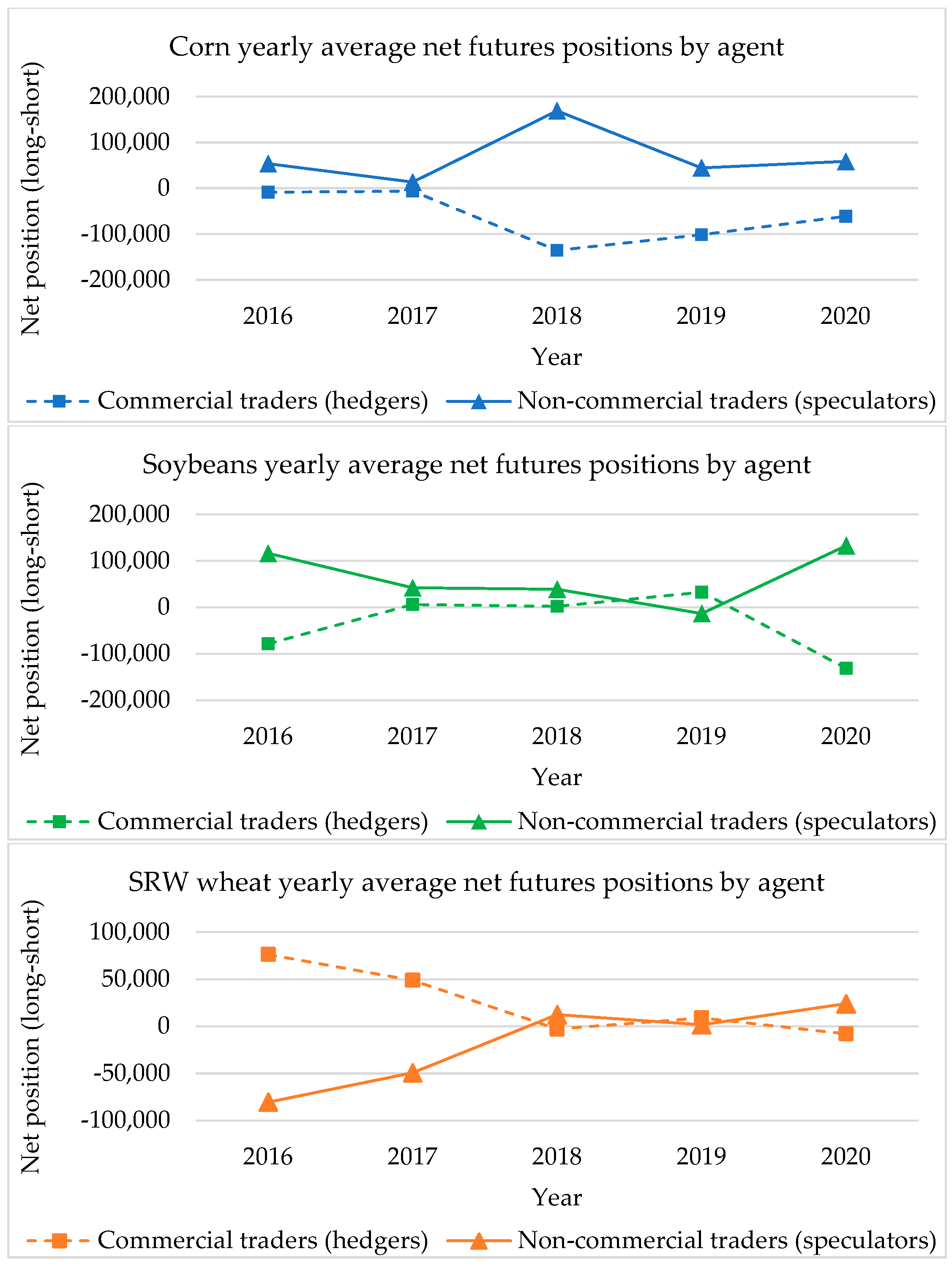
The model jointly estimates futures and expected price curves using a constant term structure of risk premiums. It is a non-stationary canonical lognormal model that allows for simultaneous estimating of both price curves.
We define Y t i as the logarithm of the spot price at time t , using the following process:
Y t i = log ( S t i ) = ( h i ) x t
where i = 1 , ,   M represents the marketing crop years. h i is a vector that relates log S t i to the P state variables common to all marketing crop years and activates for the remaining contracts a state variable at position z i = P + i 1 (index of the marketing crop year i ), which have i 1 marketing crop years to expiration. This is illustrated as follows:
h i = [ 1 1 1 P   0 1 0 M 1 ]
The total number of state variables is N = P + M 1 . The model is exponentially affine. Thus, a closed-form solution for futures and expected spot prices can be derived.
The behavior of the latent state variables is modeled according to an Ornstein–Uhlenbeck stochastic differential equation, as follows:
d x t = K x t + b d t + Σ d w t
where K is a N × N mean reversion diagonal matrix. All state variables are mean reverting except the first one, which models permanent changes in the spot price. b is a N × 1 vector containing the long-term mean values of the state variables, Σ is a N × N diagonal matrix of instantaneous volatility of state variables, and d w t is a N × 1 multivariate Wiener process with increments correlated by the N × N matrix Θ , in with each element of Θ is ρ i j   ϵ   [ 1,1 ] .
Under the equivalent martingale measure Q , the state variables use the following process:
d x t = K x t + b λ d t + Σ d w t Q
where λ is a N × 1 vector of constant risk premiums.
Under the N-factor model, it can be shown that futures prices are as follows:
F i x t , t , T = e x p x 1 t + j = 2 P e k j T t x j t + b 1 λ 1 + 1 2 σ 1 2 T t j = 2 P 1 e k j ( T t ) k j λ j + 1 2 j = 1 P l = 2 P σ j σ l ρ j l 1 e ( k j + k l ) ( T t ) k j + k l + ψ i
where
ψ i x t , t , T = 0 ,   i = 1 e k z i T t x z i t 1 e k z i T t k z i λ z i + 1 2 j = 1 P σ j σ z i ρ j z i 1 e ( k j + k z i ) ( T t ) k j + k z i ,   1 < i M
Similarly, the expected spot prices are as follows:
E t S i x t , T = e x p x 1 t + j = 2 P e k j T t x j t + b 1 + 1 2 σ 1 2 T t + 1 2 j = 1 P l = 2 P σ j σ l ρ j l 1 e ( k j + k l ) ( T t ) k j + k l + γ i
where
γ i x t , t , T = 0 ,   i = 1 e k z i T t x z i t + 1 2 j = 1 P σ j σ z i ρ j z i 1 e ( k j + k z i ) ( T t ) k j + k z i ,   1 < i M
Finally, the annual risk premiums are as follows:
π i = 1 ( T t ) l o g E t S i x t , T F i x t , t , T
Replacing the values of the expected spot price and futures price, the risk premium is as follows:
π i = λ 1 + j = 2 P 1 e k j ( T t ) k j ( T t ) λ j + ϕ i ϕ i x t , t , T =       0 ,   i = 1 1 e k z i ( T t ) k z i ( T t ) λ z i ,   1 < i M
The Kalman filter (Kalman 1960) is implemented under the incomplete data panel specification (Cortazar and Naranjo 2006), which allows state variables to be estimated even though the data series does not have observations at all discretized time steps. This is achieved by having a vector of price inputs of variable size at different stages of the model and allowing the other vectors and matrices of the measurement equation (see below) to be variable.
The Kalman filter consists of two dynamic components, which allows the Bayesian estimation of the different state variables.
The transition equation is as follows:
x t N × 1 = A t N × N x t 1 N × 1 + c t N × 1 + w t N × 1 w t ~ N ( 0 , Q t )
The measurement equation is as follows:
z t m t × 1 = H t m t × N x t N × 1 + d t m t × 1 + v t m t × 1 v t ~ N ( 0 , R t )
The transition equation relates the present time state variables to their previous status, and the measurement equation relates the observable variables (logarithm of prices) to the latent state variables.
In each stage, it must be ensured that the total number of observations is the sum between futures prices and spot price expectations (See Cortazar et al. (2019) and Cifuentes et al. (2020)), as follows:
m t N º   o b s e r v a t i o n s   a t   t = m t F N º   f u t u r e s   a t   t + m t E N º   e x p e c t e d   s p o t   a t   t

Notes

1
Initially, the Keynes–Hicks theory focused on producers as hedgers shorting futures to manage crop price risks, with speculators taking long positions for a risk premium. This theory was later expanded to allow hedgers and speculators to assume long or short positions in futures markets.
2
There may also be risk premium transfers between hedgers to hedgers, speculators to speculators, and speculators to hedgers, but the theory of net hedging pressure focuses on the market’s net positions.
3
However, the proposed model benefits from having more factors and parameters.
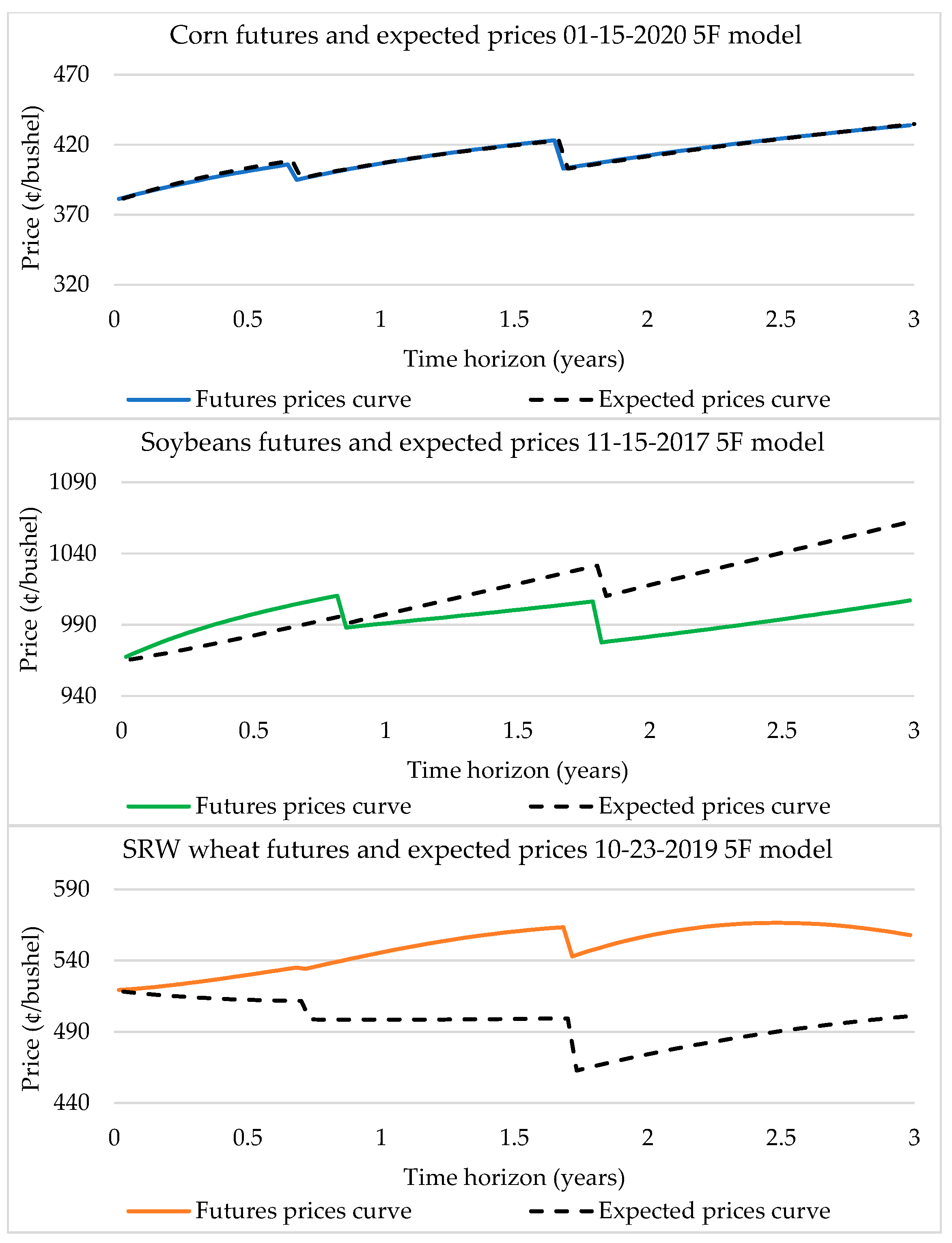
4
Similar results are obtained for soybeans and SRW wheat.

References

  1. Aït-Youcef, Camille. 2019. How index investment impacts commodities: A story about the financialization of agricultural commodities. Economic Modelling 80: 23–33. [Google Scholar] [CrossRef]
  2. Aglasan, Serkan, Roderick M. Rejesus, Stephen Hagen, and William Salas. 2023. Cover Crops, Crop Insurance Losses, and Resilience to Extreme Weather Events. American Journal of Agricultural Economics 106: 1–25. [Google Scholar] [CrossRef]
  3. Bakshi, Gurdip, Xiaohui Gao, and Alberto G. Rossi. 2019. Understanding the Sources of Risk Underlying the Cross Section of Commodity Returns. Management Science 65: 619–41. [Google Scholar] [CrossRef]
  4. Basu, Devraj, and Joëlle Miffre. 2013. Capturing the risk premium of commodity futures: The role of hedging pressure. Journal of Banking & Finance 37: 2652–64. [Google Scholar]
  5. Beck, Stacie E. 1993. A Rational Expectations Model of Time Varying Risk Premia in Commodities Futures Markets: Theory and Evidence. International Economic Review 34: 149–68. [Google Scholar] [CrossRef]
  6. Beck, Stacie E. 1994. Cointegration and Market Efficiency in Commodities Futures Markets. Applied Economics 26: 249–57. [Google Scholar] [CrossRef]
  7. Beckmann, Joscha, and Robert Czudaj. 2014. Non-linearities in the relationship of agricultural futures prices. European Review of Agricultural Economics 41: 1–23. [Google Scholar] [CrossRef]
  8. Boyd, Naomi E., Jeffrey H. Harris, and Bingxin Li. 2018. An update on speculation and financialization in commodity markets. Journal of Commodity Markets 10: 91–104. [Google Scholar] [CrossRef]
  9. Brignoli, Paolo Libenzio, Alessandro Varacca, Cornelis Gardebroek, and Paolo Sckokai. 2024. Machine learning to predict grains futures prices. Agricultural Economics 55: 479–97. [Google Scholar] [CrossRef]
  10. Cifuentes, Sebastián, Gonzalo Cortazar, Hector Ortega, and Eduardo S. Schwartz. 2020. Expected prices, futures prices and time-varying risk premiums: The case of copper. Resources Policy 69: 101825. [Google Scholar] [CrossRef]
  11. CME Group. 2024. Comparing New Crop and Old Crop Risk. Available online: https://www.cmegroup.com/articles/2023/new-crop-vs-old-crop-risk-of-the-past-year.html (accessed on 8 November 2024).
  12. Cortazar, Gonzalo, and Lorenzo Naranjo. 2006. An N-Factor Gaussian Model Of Oil Futures Prices. The Journal of Futures Markets 26: 243–68. [Google Scholar] [CrossRef]
  13. Cortazar, Gonzalo, Cristobal Millard, Hector Ortega, and Eduardo S. Schwartz. 2019. Commodity Price Forecasts, Futures Prices, and Pricing Models. Management Science 65: 4141–55. [Google Scholar] [CrossRef]
  14. Cortazar, Gonzalo, Hector Ortega, Maximiliano Rojas, and Eduardo S. Schwartz. 2021. Commodity index risk premium. Journal of Commodity Markets 22: 100156. [Google Scholar] [CrossRef]
  15. Cortazar, Gonzalo, Philip Liedtke, Hector Ortega, and Eduardo S. Schwartzd. 2022. Time-Varying Term Structure of Oil Risk Premia. The Energy Journal 43: 571–91. [Google Scholar] [CrossRef]
  16. Dutt, Hans R., and John Fenton. 1997. Crop Year Influences and Variability of the Agricultural Futures Spreads. The Journal of Futures Markets 17: 341–67. [Google Scholar] [CrossRef]
  17. Fainé, Francisco Ignacio Fainé. 2010. Modelación Estocástica Multifactorial de los Precios Futuros de Commodities Agrícolas y su Estimación Mediante el Filtro de Kalman. Master’s thesis, Pontificia Universidad Católica de Chile, Santiago, Chile. Available online: https://repositorio.uc.cl/xmlui/handle/11534/1868 (accessed on 8 November 2024).
  18. Fama, Eugene F., and Kenneth R. French. 1987. Commodity Futures Prices: Some Evidence on Forecast Power, Premiums, and the Theory of Storage. The Journal of Business 60: 55–73. [Google Scholar] [CrossRef]
  19. Frank, Julieta, and Philip Garcia. 2009. Time-varying risk premium: Further evidence in agricultural futures markets. Applied Economics 41: 715–25. [Google Scholar] [CrossRef]
  20. French, Kenneth R. 1986. Detecting Spot Price Forecasts In Futures Prices. The Journal of Business 59: S39–S54. [Google Scholar] [CrossRef]
  21. Gorton, Gary B., Fumio Hayashi, and K. Geert Rouwenhorst. 2012. The Fundamentals of Commodity Futures Returns. Review of Finance 17: 35–105. [Google Scholar] [CrossRef]
  22. Hevia, Constantino, Ivan Petrella, and Martin Sola. 2018. Risk premia and seasonality in commodity futures. Journal of Applied Econometrics 33: 853–73. [Google Scholar] [CrossRef]
  23. Hicks, John Richard. 1939. Value and Capital: An Inquiry into Some Fundamental Principles of Economic Theory. Oxford: Clarendon Press. [Google Scholar]
  24. Hirshleifer, David. 1990. Hedging pressure and futures price movements in a general equilibrium model. Econometrica: Journal of the Econometric Society 58: 411–28. [Google Scholar] [CrossRef]
  25. Huang, Joshua, Teresa Serra, and Philip Garcia. 2020. Are futures prices good price forecasts? Underestimation of price reversion in the soybean complex, European Review of Agricultural Economics 47: 178–99. [Google Scholar] [CrossRef]
  26. Irwin, Scott H., and Dwight R. Sanders. 2012. Financialization and Structural Change in Commodity Futures Markets. Journal of Agricultural and Applied Economics 44: 371–96. [Google Scholar] [CrossRef]
  27. Kaldor, Nicholas. 1939. Speculation and Economic Stability. The Review of Economic Studies 7: 1–27. [Google Scholar] [CrossRef]
  28. Kalman, Rudolph Emil. 1960. A New Approach to Linear Filtering and Prediction Problems. Transactions of the ASME–Journal of Basic Engineering 82: 35–45. [Google Scholar] [CrossRef]
  29. Karali, Berna, Scott H. Irwin, and Olga Isengildina-Massa. 2020. Supply Fundamentals and Grain Futures Price Movements. American Journal of Agricultural Economics 102: 548–68. [Google Scholar] [CrossRef]
  30. Keynes, John Maynard. 1930. A Treatise on Money. The Applied Theory of Money. London: Macmillan and Co., vol. 2. [Google Scholar]
  31. Koekebakker, Steen, and Gudbrand Lien. 2004. Volatility and Price Jumps in Agricultural Futures Prices-Evidence from Wheat Options. American Journal of Agricultural Economics 86: 1018–31. [Google Scholar] [CrossRef]
  32. Kolb, Robert W. 1992. Is normal backwardation normal? Journal of Futures Markets 12: 75–91. [Google Scholar] [CrossRef]
  33. Li, Jian, and Jean-Paul Chavas. 2023. A dynamic analysis of the distribution of commodity futures and spot prices. American Journal of Agricultural Economics 105: 122–43. [Google Scholar] [CrossRef]
  34. Mitra, Sophie, and Jean-Marc Boussard. 2012. A simple model of endogenous agricultural commodity price fluctuations with storage. Agricultural Economics 43: 1–15. [Google Scholar] [CrossRef]
  35. Ordu, Beyza Mina, Adil Oran, and Ugur Soytas. 2018. Is food financialized? Yes, but only when liquidity is abundant. Journal of Banking and Finance 95: 82–96. [Google Scholar] [CrossRef]
  36. Pérez Zañartu, José Antonio. 2023. Risk Premium Structure of Agricultural Commodities. Master’s thesis, Pontificia Universidad Católica de Chile, Santiago, Chile. [Google Scholar]
  37. Prager, Daniel, Christopher Burns, Sarah Tulman, and James MacDonald. 2020. Farm Use of Futures, Options, and Marketing Contracts; EIB-219. Washington, DC: U.S. Department of Agriculture, Economic Research Service, pp. 1–33. [CrossRef]
  38. Sanders, Dwight R., and Scott H. Irwin. 2010. A speculative bubble in commodity futures prices? Cross-sectional evidence. Agricultural Economics 41: 25–32. [Google Scholar] [CrossRef]
  39. Scheinkman, Jose A., and Jack Schechtman. 1983. A Simple Competitive Model with Production and Storage. The Review of Economic Studies 50: 427–41. [Google Scholar] [CrossRef]
  40. Sørensen, Carsten. 2002. Modeling seasonality in agricultural commodity futures. The Journal of Futures Markets 22: 393–426. [Google Scholar] [CrossRef]
  41. Telser, Lester G. 1958. Futures Trading and the Storage of Cotton and Wheat. Journal of Political Economy 66: 233–55. [Google Scholar] [CrossRef]
  42. Tokgoz, Simla, Wei Zhang, Siwa Msangi, and Prapti Bhandary. 2012. Biofuels and the future of food: Competition and complementarities. Agriculture 2: 414–35. [Google Scholar] [CrossRef]
  43. USDA. 2022a. Data Products, Wheat Data; September 8, Retrieved from Documentation. Available online: https://www.ers.usda.gov/data-products/wheat-data/documentation/ (accessed on 8 November 2024).
  44. USDA. 2022b. Farm Practices & Management, Risk Management; June 16, Retrieved from Risk in Agriculture. Available online: https://www.ers.usda.gov/topics/farm-practices-management/risk-management (accessed on 8 November 2024).
  45. Vollmer, Teresa, Helmut Herwartz, and Stephan von Cramon-Taubadel. 2020. Measuring price discovery in the European wheat market using the partial cointegration approach. European Review of Agricultural Economics 47: 1173–200. [Google Scholar] [CrossRef]
  46. Working, Holbrook. 1948. Theory of the Inverse Carrying Charge in Futures Markets. Journal of Farm Economics 30: 1–28. [Google Scholar] [CrossRef]
Figure 1. Deviations of the average contract price from the crop year average price. Source: data from Bloomberg.
Risks 13 00009 g001aRisks 13 00009 g001b
Figure 2. Corn, soybeans, and SRW wheat futures prices from 2016 to 2021. Source: Bloomberg.
Risks 13 00009 g002
Figure 3. Corn, soybeans, and SRW wheat analysts’ forecasts from 2016 to 2021 (Bloomberg).
Risks 13 00009 g003
Figure 4. Futures price curves for three alternative models on a given date.
Risks 13 00009 g004
Figure 5. Futures and expected price curves on a given date as examples of model outputs.
Risks 13 00009 g005
Figure 6. Commodity risk premium term structure by crop year and horizon.
Risks 13 00009 g006
Figure 7. Yearly average of net positions (long–short) by type of market player. Source: Commitments of Traders futures only reports, CFTC.
Risks 13 00009 g007
Table 1. Usual planting and harvesting dates in the United States.
CommodityJanFebMarAprMayJunJulAugSepOctNovDec
Corn PP HHH
Soybeans PP HH
SRW wheat HH PP
PPlant Mid-seasonHHarvest
Source: National Agricultural Statistics Service, USDA.
Table 2. Corn, soybeans, and SRW futures data from 2016 to 2020, by marketing crop year. The table includes mean price, price standard deviation, maximum price, minimum price, mean price, and number of observations for corn, soybeans, and SRW wheat for each marketing crop year.
Corn
Marketing cropMean pricePrice SDMax priceMin priceMean maturityNumber of
year (i)(¢/bushel) (¢/bushel)(¢/bushel)(years)observations
1377.2324.24474.50304.500.3175582
2397.2224.48461.75315.501.05551044
3409.4515.91440.00359.501.9980913
Soybeans
Marketing cropMean pricePrice SDMax priceMin priceMean maturityNumber of
year (i)(¢/bushel) (¢/bushel)(¢/bushel)(years)observations
1969.5483.501303.75814.250.3426884
2961.5455.701150.25827.751.06351566
3952.8240.281032.00831.752.00941398
SR Wheat
Marketing cropMean pricePrice SDMax priceMin priceMean maturityNumber of
year (i)(¢/bushel) (¢/bushel)(¢/bushel)(years)observations
1493.7157.21640.75361.000.3169542
2529.5341.46641.50428.501.01611044
3557.5928.54632.75487.252.01631044
Source: Bloomberg.
Table 3. Analysts’ forecasts data from 2016 to 2020 by marketing crop year (Bloomberg). The table includes mean price, price standard deviation, maximum price, minimum price, mean price, and number of observations for corn, soybeans, and SRW wheat for each marketing crop year.
Corn
Marketing cropMean pricePrice SDMax priceMin priceMean maturityNumber of
year (i)(¢/bushel) (¢/bushel)(¢/bushel)(years)observations
1380.8925.38510.00325.000.4545257
2394.1725.31500.00325.000.9949643
3414.2528.75500.00363.001.9635246
Soybeans
Marketing cropMean pricePrice SDMax priceMin priceMean maturityNumber of
year (i)(¢/bushel) (¢/bushel)(¢/bushel)(years)observations
1969.6367.451440.00825.000.4522266
2969.0963.021600.00820.000.9879668
3997.6663.341200.00875.001.9653248
SR Wheat
Marketing cropMean pricePrice SDMax priceMin priceMean maturityNumber of
year (i)(¢/bushel) (¢/bushel)(¢/bushel)(years)observations
1481.1742.09650.00351.000.4851313
2480.8245.17680.00265.261.0302711
3486.0556.91711.00260.591.9643306
Table 4. Mean absolute percentage errors for the 5F, 3F, and 3F with seasonality models—time window data between 2016 and 2020 (in-sample) and 2021 (out-of-sample).
ModelCommodityMAPEMAPENº of ParametersLog-Likelihood
In-SampleOut-of-Sample
5FCorn0.12820.35472612,273
Soybeans0.21350.40922618,543
SRW wheat0.21200.24982611,731
3FCorn0.66542.1468139809
Soybeans0.53141.06441315,974
SRW wheat0.46420.79861310,777
3F with seasonalityCorn0.39291.65031710,761
Soybeans0.37090.75621717,100
SRW wheat0.38130.62511711,181
Table 5. Corn: Parameters for the 5F model. Standard deviation, t-statistic, and p-value. Significance levels are given by *** 1%, ** 5%, and * 10%.
Corn
ParameterEstimateDeviationt-Statisticp-Value
k 2 1.2879 ***0.032639.4480
k 3 1.2428 ***0.029741.8040
k 4 1.0033 ***0.079612.6100
k 5 0.6799 ***0.050013.5990
λ 1 0.00850.01170.72850.3054
λ 2 1.20321.11301.08110.2220
λ 3 −1.18491.1141−1.06360.2262
λ 4 −0.0079 *0.0044−1.77540.0827
λ 5 −0.00600.0042−1.42130.1452
ρ 12 −0.6151 ***0.1060−5.80420
ρ 13 0.6215 ***0.10495.92290
ρ 14 0.00730.12340.05900.3979
ρ 15 −0.03400.1037−0.32790.3776
ρ 23 −0.9998 ***0.0001−108540
ρ 24 0.3110 ***0.10462.97300.0051
ρ 25 0.5136 ***0.11924.30790
ρ 34 −0.3140 ***0.1036−3.03050.0043
ρ 35 −0.5106 ***0.1186−4.30330.0001
ρ 45 0.3147 ***0.11392.76320.0091
σ 1 0.0671 ***0.004614.7010
σ 2 4.9349 ***1.48873.31490.0018
σ 3 5.0632 ***1.48673.40560.0013
σ 4 0.0767 ***0.00789.89500
σ 5 0.2065 ***0.018810.9860
b 1 0.0249 **0.01182.11020.0435
ξ F 0.0024 ***0.0000139.770
ξ E 0.0680 ***0.0006107.570
Log-likelihood14,772
Table 6. Mean absolute percentage error (MAPE) for the 5F model for corn, soybeans, and SRW wheat. Data between 2016 and 2020 (in-sample) and 2021 (out-of-sample).
DataCommodityMAPEMAPE
In-SampleOut-of-Sample
Corn0.13170.3847
Futures pricesSoybeans0.21470.4046
SRW wheat0.21420.2275
Corn5.132910.2856
Expected pricesSoybeans4.206114.4784
SRW wheat7.759211.7089
Disclaimer/Publisher’s Note: The statements, opinions and data contained in all publications are solely those of the individual author(s) and contributor(s) and not of MDPI and/or the editor(s). MDPI and/or the editor(s) disclaim responsibility for any injury to people or property resulting from any ideas, methods, instructions or products referred to in the content.

