Abstract
In this paper, we carry out a comprehensive comparison of Gaussian generalized autoregressive conditional heteroskedasticity (GARCH) and autoregressive stochastic volatility (ARSV) models for volatility forecasting using the S&P 500 Index. In particular, we investigate their performance using the physical measure (also known as the real-world probability measure) for risk management purposes and risk-neutral measures for derivative pricing purposes. Under the physical measure, after fitting the historical return sequence, we calculate the likelihoods and test the normality for the error terms of these two models. In addition, two robust loss functions, the MSE and QLIKE, are adopted for a comparison of the one-step-ahead volatility forecasts. The empirical results show that the ARSV(1) model outperforms the GARCH(1, 1) model in terms of the in-sample and out-of-sample performance under the physical measure. Under the risk-neutral measure, we explore the in-sample and out-of-sample average option pricing errors of the two models. The results indicate that these two models are considerably close when pricing call options, while the ARSV(1) model is significantly superior to the GARCH(1, 1) model regarding fitting and predicting put option prices. Another finding is that the implied versions of the two models, which parameterize the initial volatility, are not robust for out-of-sample option price predictions.
1. Introduction
In financial risk management, there can never be too much emphasis on monitoring market volatility. Market volatility rises, as does the risk of collapse. The stock market crash on 19 October 1987, the tech bubble burst in the late 1990s, the global financial crisis in 2008, the stock plunge on 5 February 2018, and the pandemic related stock plunges in March 2020 are all examples of such a knock-on effect. As a crucial parameter when pricing derivatives and estimating measures of risk, how to precisely estimate and forecast market return volatilities has been an enduringly popular field of research.
There are three prevalent types of volatility models: (1) the ARCH/GARCH-family models (Bollerslev 1986; Engle 1982; Engle and Ng 1993), (2) stochastic volatility (SV) models (e.g., the autoregressive stochastic volatility (ARSV) model (Taylor 1982), the Hull–White model (Hull and White 1987), and the multi-factor model (Dahlen and Solibakke 2012)), and (3) realized volatility (RV) models (Andersen et al. 2001). RV models depend on high-frequency intra-daily data which are not always available. Therefore, we only consider the first two types of models. In particular, we focus on the two most popular models among their classes, namely the Gaussian GARCH(1, 1) and ARSV(1) models. The fundamental difference between these two models is that in the ARSV(1) model, the volatility is treated as a latent variable with unexpected noise, while the volatility in the GARCH(1, 1) model is deterministic.
Despite the extra adaptability, the latent volatility process in the SV models adds to the difficulty of parameter estimation. Due to breakthroughs in computing capacity, along with more efficient estimation methods, taking advantage of SV models is increasingly likely. When faced with the choice between the ARCH/GARCH-family models and SV models, people are interested in which one gives a more accurate volatility estimate. Carnero et al. (2001) show the ARSV(1) model is more flexible than the GARCH(1, 1) model regarding excess kurtosis, low first-order autocorrelation, and high persistence of volatility. Yu (2002) makes a comparison of nine models in terms of predicting volatilities using New Zealand stock data and demonstrates that the ARSV(1) model outperforms its rival candidates. Furthermore, Lehar et al. (2002) compare the performance of the GARCH and Hull–White models in terms of their out-of-sample option valuation errors and Value-at-Risk forecasts. Moreover, the ability to reproduce the stylized facts in the financial series of the GARCH(1, 1), exponential GARCH(1, 1), and ARSV(1) models is investigated by Malmsten and Teräsvirta (2010), and they conclude that none of the models dominates over the others.
Generally speaking, volatility measures are classified into two main categories. The first is the physical measure, under which the volatilities are directly tracked via fitting series of the historical asset returns. This measure, also known as the real-world measure, is usually applied in portfolio hedging and risk management. For example, Skoglund et al. (2010) validate Value-at-Risk (VaR) models using historical stock data and show that GARCH volatility models are effective in the VaR models. The other is the risk-neutral measure, under which the volatilities of the underlying asset are derived from its derivative prices. Naturally, the risk-neutral measure is suitable for option pricing. The local risk-neutral valuation relationship assumes that the volatilities under the two measures above are equal (see Duan (1995)). In practice, the risk-neutral measure, however, tends to have larger volatilities than the counterparts under the physical measure, which is known as the volatility risk premium phenomenon (see Bakshi and Kapadia (2003); Low and Zhang (2005)). Explanations for such a phenomenon are beyond the scope of this paper. In this paper, we only consider the two models’ performance under these two volatility measures.
To the best of our knowledge, risk-neutral GARCH(1, 1) and ARSV(1) models have not been compared in previous empirical studies. This paper complements the literature by conducting a comprehensive comparison of the GARCH(1, 1) and ARSV(1) models regarding their in-sample fitting and out-of-sample prediction capabilities using both physical and risk-neutral measures. Under the physical measure, we calculate their log-likelihoods, test the normality of the error term, and explore the one-step-ahead volatility forecasts. Under the risk-neutral measure, we investigate the option pricing errors of the original and implied versions of the two models.
The rest of this paper is organized as follows: In Section 2, we discuss the parameter estimation methods for the GARCH(1, 1) and ARSV(1) models under both the physical and risk-neutral measures. In Section 3, we describe the dataset and discuss the methodologies used for a comprehensive comparison of these two models. Then, we investigate the empirical results in Section 4. In Section 5, we conclude this paper by suggesting potential topics for future research. We give all of the technical details in the Appendix A, Appendix B and Appendix C.
2. The Models and Parameter Estimation Methods
In what follows, we will discuss the parameter estimation for both the GARCH(1, 1) and ARSV(1) models under the physical and risk-neutral measures, respectively.
2.1. Estimating the GARCH(1, 1) Model Under the Physical Measure
A volatility model under the physical measure is estimated to fit the return series as precisely as possible. The GARCH(1, 1) model, which relates the current conditional variance to the lagged squared residual and the lagged conditional variance estimate, is constructed as shown in Equation (1):
where denotes the log daily return series (which can be magnified), and stands for the conditional variance estimate at time t. To ensure the stationarity of the variance, the parameters are required to satisfy , and .
Since follows a normal distribution, the maximum-likelihood estimation method can be adopted to estimate the GARCH(1, 1) model under the physical measure. Suppose is its constant parameter vector to be estimated. Given a sample of T original/magnified log daily returns, the GARCH(1, 1) model under the physical measure is estimated by maximizing its log-likelihood function, denoted by , as follows:
2.2. Estimating the ARSV(1) Model Under the Physical Measure
There have been many studies on Taylor’s ARSV model. Actually, in Bayesian time series analysis, ARSV is a fundamental example when studying Markov chain Monte Carlo (MCMC) algorithms or particle filter (also known as Sequential Monte Carlo) methods since its nonlinearity makes traditional Kalman filtering infeasible. Generally, there are two equivalent forms of the ARSV(1) model (see Appendix A). The first form assumes that the latent log variance follows a Gaussian AR(1) process with a constant return drift. In this paper, we adopt the following ARSV(1) model because it is easier to estimate and more straightforward to implement in the option pricing model:
where is still the original/magnified log daily return series, and denotes the conditional variance at time t. Suppose is the constant parameter vector of the ARSV(1) model under the physical measure. The scale parameter replaces the constant drift of the log variance process. For the persistence parameter , should be ensured to satisfy the stationarity condition. In addition, and are two independent processes in this paper, though in many cases they are assumed to be correlated in order to capture the leverage effect.
Unlike the GARCH(1, 1) model, the log variance process in the ARSV(1) model includes an unexpected noise term, which explains why it is classified as a stochastic volatility model. Despite the absence of an analytical likelihood function, Monte Carlo simulation methods have been proposed for estimating the ARSV(1) model. MCMC algorithms such as the Gibbs sampler (Kalaylıoğlu and Ghosh 2009) suggest the posterior distributions of the parameters. Such algorithms are faced with prior density selection issues and have high time consumption after the burn-in period. On the other hand, particle filter is effective for estimating the likelihood, and the expectation-maximization (EM) or gradient ascent method can subsequently be implemented to maximize the estimated likelihood. Particle MCMC (Andrieu et al. 2010), a combination of the particle filter and MCMC methods, can also be used for the parameter learning of the ARSV(1) model, though it is quite time-consuming.
In this paper, particle filter is preferred to MCMC algorithms when estimating the ARSV(1) model under the physical measure because the former naturally derives the approximate likelihood that is necessary for the model comparison. Moreover, since the ARSV(1) model belongs to the exponential family, we adopt a forward-only version of the Forward Filter Backward Smoothing (FFBS) algorithm with the EM method (Del Moral et al. 2010) to maximize the particle-based likelihood of the ARSV(1) model (see Appendix B).
2.3. Estimating the Models Under the Risk-Neutral Probability Measure
Instead of maximizing the likelihood, parameter estimation under the risk-neutral measure is directly related to option pricing. Duan (1995) suggests that the risk-neutral GARCH(1, 1) model be given by
where denotes the daily risk-free interest rate, denotes the volatility estimate at time t, and denotes the asset spot price. Similar to its counterpart under the physical measure, the risk-neutral ARSV(1) model can be derived as follows:
where stands for the volatility estimate at time t. For a European call/put option, its price at time t is calculated as the discounted average pay-off at maturity T under the risk-neutral measure Q:
where K is its strike price, is the asset price at maturity T, and is a filtration. The time unit in Equation (6) is one trading day. Without an analytical solution for the option price for both the risk-neutral GARCH(1, 1) and ARSV(1) models, the options need to be priced using Monte Carlo simulation. Let the initial volatility estimate at time t be . Based on Equation (4), the asset price at maturity T under the risk-neutral GARCH(1, 1) model is computed through a simulated return process step by step (the log variance at each time step is simultaneously determined) as follows:
where the superscript G stands for the GARCH(1, 1) model. Repeating the simulation m times, the European call/put option price at time t of the risk-neutral GARCH(1, 1) model is given by
where is the GARCH(1, 1) parameter vector, and j denotes the simulation index.
On the other hand, the risk-neutral ARSV(1) model has a volatility process that is independent of the return dynamics. Since the initial volatility estimate is , the initial is set to . Conditional on one simulated sequence, the European option price of the risk-neutral ARSV(1) model at time t can be calculated using the Black–Scholes (B-S) formula as follows:
For completeness and quick reference, we also give the B-S formula here.
where
We still adopt the trading day time unit for the parameters of the B-S formula, and the superscript A stands for the ARSV(1) model. Despite the commonly used yearly expressed parameters in the B-S formula, the daily expressed ones actually work in the same way. In other words, if T, t, , and are all expressed in ‘day’, and Y ( in this paper) is the number of trading days in a year. The proof for Equations (9) and (10) is straightforward.
Proof.
Suppose the sequence has been obtained. We have
where stands for the operator for ‘equivalence in distribution’. As for , we have according to the properties of the normal distribution. Hence, with defined in Equation (11), we can simplify Equation (14) by
It is obvious that Equation (15) can be seen as a model in which the asset price follows a geometric Brownian motion with the constant daily volatility and the constant daily risk-free rate . In fact, the B-S formula is derived from such a model. Therefore, we have
□
Then, the simulated European call option price in the risk-neutral ARSV(1) model is derived by
where is computed from the j-th simulation path of the ARSV(1) log variance process with a given parameter vector . In this paper, the simulation number m is set to , and the common random number technique is adopted to price options with different strike prices. Similarly, the European put option can be valued by
As Equations (16) and (17) show, all we need to simulate is the log variance dynamics when pricing options under the risk-neutral ARSV(1) model even though it originally has two innovation processes. On the other hand, the conditional variance process in the risk-neutral GARCH(1, 1) model is deterministic and fully depends on the previous return. That is why only the return dynamics needs to be simulated in the GARCH(1, 1) option pricing model.
Suppose we have a collection of options with their observed market prices. As for both the risk-neutral GARCH(1, 1) and ARSV(1) models, the nonlinear-least-squares parameter estimator is obtained by minimizing the mean squared pricing error (MSPE):
where is the observed market price of the i-th option, n is the number of options in the collection, and is the theoretical price of the i-th option derived from the corresponding volatility model using the parameter vector .
Remark 1.
Apparently, the accuracies of the approximations in (8), (16), and (17) depend on the value of m. For different products, the convergence speeds can be different. In this paper, our main focus is a comparison of the converged values under GARCH (1, 1) and ARSV(1) instead of a comparison of the convergence speed; we simply choose a large value of m (m = 10,000) for both the GARCH(1, 1) and ARSV(1) methods.
3. Methodology and Data
3.1. Comparison Under the Physical Measure
We estimate a volatility model under the physical measure by maximizing its log-likelihood. The log-likelihood of the GARCH(1, 1) model is straightforwardly calculated, while that in the ARSV(1) model needs to be computed via particle filter. Since both of the two models have three parameters, the maximum likelihood is valuable for the in-sample fitting comparison.
Furthermore, some other statistics can be compared using the estimated volatility at each time step. For the GARCH(1, 1) model, given the parameter estimates under the physical measure and the observed return series, we can fully determine the sequence of conditional variances. On the other hand, for the ARSV(1) model, its conditional variance remains a latent state variable, even though its parameter estimates have been obtained. Let the estimated parameter vector of the ARSV(1) model be and the size of the in-sample dataset be T. Using particle smoothing algorithms (see Appendix C.2), the particle-based volatility estimate, , is approximated for using Equation (A15). Subsequently, through normality tests such as the Kolmogorov–Smirnov, Lilliefors, and Anderson–Darling tests, we can investigate how good the error sequence ( for the GARCH(1, 1) model and for the ARSV(1) model) is for fitting the assumed standard normal distribution.
As for any volatility model, fitting the in-sample observations is one task while forecasting volatilities in the future is an entirely different challenge. The preferred model for an in-sample comparison does not necessarily guarantee a better out-sample forecast. Patton (2011) studies the properties of well-documented loss functions developed for volatility forecast evaluation and shows that only the MSE and QLIKE, defined in Equations (19) and (20), are robust to noisy volatility proxies. Therefore, in this paper, we use these two loss functions for the out-of-sample one-step-ahead volatility forecast comparison between the two volatility models.
where n is the number of out-of-sample observations, is the conditional variance forecast for time t given the information set until time , and is the true conditional variance or the conditionally unbiased variance proxy at time t. In practice, the true conditional variances are unobservable, and the realized volatility, computed by the sum of intra-daily returns, is often considered to be a good proxy. Though such computation is not complicated, high-frequency intra-daily return data are not always accessible. The variance proxy suggested by Awartani and Corradi (2005), which adopts the squared filtered daily return and ensures the correct ranking of the volatility forecast models, is adopted in this paper. In Equations (19) and (20), is replaced with , where is the out-of-sample log daily return and denotes the mean of the out-of-sample log daily returns.
3.2. Comparison Under the Risk-Neutral Measure
The risk-neutral versions of the GARCH(1, 1) and ARSV(1) models will be evaluated based on in-sample option price fitting and out-of-sample option price prediction. Instead of handling a collection of options over a long time span, we analyze the options in a single day, a choice adopted by Bakshi et al. (1997), for the following reasons. Firstly, while the options limited to a single day might not be sufficient for a robust parameter estimation, it indeed eases the computational burden when minimizing the in-sample pricing error. Moreover, one-day collection makes more sense because the parameter estimation is updated as soon as new information arrives, while a long-term sample has to assume that the parameters stay unchanged for a long time. This choice also avoids mixing up known information with unknown conditions. For example, if the collection includes the options from two different days, we have to ignore the asset price on the second day when pricing the first-day options, even though that information is provided.
Another issue is the selection of the out-of-sample options. After estimating the parameters by minimizing the in-sample option pricing error, we use them to calculate the pricing error of the out-of-sample options, which indicates the model’s capability of predicting option prices in the future. Indeed, the out-of-sample performance draws much more attention in the derivative market. A smaller in-sample option pricing error indicates that a model fits the observed option prices better, but it is the out-of-sample prediction that guides participants’ behaviors. Christoffersen and Jacobs (2004) value options for the next Wednesday using parameters estimated from the current Wednesday when comparing different GARCH models. This is a favorable choice because it leaves five days for the parameter updates. As previously demonstrated, the new observed asset prices will directly affect the deterministic conditional variance in the GARCH(1, 1) model. However, leaving several days between the in-sample and out-of-sample collections is trivial for the ARSV(1) model because in that model, the new price information will not be involved in the log variance dynamics, which is stochastic and independent of the return process. Therefore, in this paper, the out-of-sample options come from the day following the in-sample single day.
Moreover, a precondition for estimating the risk-neutral parameters is obtaining an initial volatility estimate. Suppose the in-sample options are selected from Day t and the out-of-sample options come from the next day—Day . In this paper, the initial volatility estimate for Day t, denoted by , is initialized to the standard deviation of the unconditional sample of the 180-day log returns before Day t, and the volatility estimates after Day t are updated based on the corresponding volatility model. We also investigate the results after parameterizing the initial volatility. When the risk-neutral parameters for Day t are estimated by minimizing the in-sample MSPE using Equation (18), they are assumed to stay unchanged overnight. Hence, the out-of-sample option pricing errors on Day are valued under the corresponding volatility model using its in-sample parameter estimates, the initial volatility estimate for Day t, and the new information set on Day . Moreover, we assume a constant daily risk-free interest rate of .
3.3. Data
This paper focuses on the daily close value and options of the S&P 500 Index. For the comparison under the physical measure, the in-sample observations (Sample A) consist of the log daily return sequence over a ten-year period from 2 January 1996 to 30 December 2005. When estimating the in-sample MLE parameters analytically (GARCH) or numerically (ARSV), we use the magnified return series, (), obtained by scaling the original log daily returns by 100. In addition, 250 log daily returns, magnified in the same way, following Sample A constitute the out-of-sample dataset—Sample B. A summary of Sample A and Sample B is presented in Table 1.

Table 1.
Characteristics of the magnified in-sample (Sample A) and out-of-sample (Sample B) datasets under the physical measure.
For the comparison under the risk-neutral measure, as previously mentioned, the ‘one day in-sample with the second day out-of-sample’ rule is adopted. During the period of 30 October 2017 to 1 February 2018, all of the in-sample and out-of-sample pairs are chosen from every two consecutive days in each week; that is, we have four such pairs every week. For example, every Monday will only be selected as the in-sample day, and the following Tuesday will be its out-of-sample ‘partner’. That Tuesday itself also offers the second in-sample option, while its matched out-of-sample day is the following Wednesday, and so on. We skip holidays and avoid selecting Friday as an in-sample day so that there is no weekend gap between the in-sample and out-of-sample pair. For each day, around thirty-five options with the highest volumes whose index-to-strike ratio is located in are selected, and the market price of each chosen option is set as the mean value of the last bid and the ask prices when the market closes.
4. The Empirical Study
4.1. Results Under the Physical Measure
4.1.1. In-Sample Comparison Under the Physical Measure
The parameter estimates of the GARCH(1, 1) and ARSV(1) models for Sample A under the physical measure are listed in Table 2, in which ‘LL’ is short for log-likelihood and the standard errors are reported in parentheses . The parameter estimates and their standard errors in the ARSV(1) model are the sample mean and sample standard deviations of the estimates of the last 250 iterations using the offline EM method. This shows the ARSV(1) model has a larger log-likelihood.
Table 2.
Parameter estimates under the physical measure, Sample A.
When calculating the maximum-likelihood estimators (MLE) with the GARCH(1, 1) model, the initial volatility for Day 1 (the first in-sample day), denoted by , is set as the standard deviation of Sample A. The subsequent conditional variances are updated by the model. In the s-th EM offline iteration for estimating the ARSV(1) model, we also set a prior normal distribution for the particles for Day 1 such that the expected volatility on that day is same as . Hence, the prior distribution can be derived as follows:
We assume in the s-th iteration for where N is the number of particles. The parameter estimate of the s-th iteration is updated from the maximum step of the -th iteration. One popular choice for is . Here, we set to ensure the diversity of the particles. is calculated by solving , as in Equation (21):
Table 2 shows that the maximum-likelihood estimates of the GARCH(1, 1) model under the physical measure, whose p-values are all less than 0.01, are significantly different from 0. Many empirical studies have a positive log-likelihood because their returns are not subject to 100 times magnification. Revisiting the second equation in Equation (2), when magnifying and at the same time, the first term and the third term stay unchanged, while the second term is indeed affected. A larger sequence of conditional variance estimates may decrease the log-likelihood to a negative value.
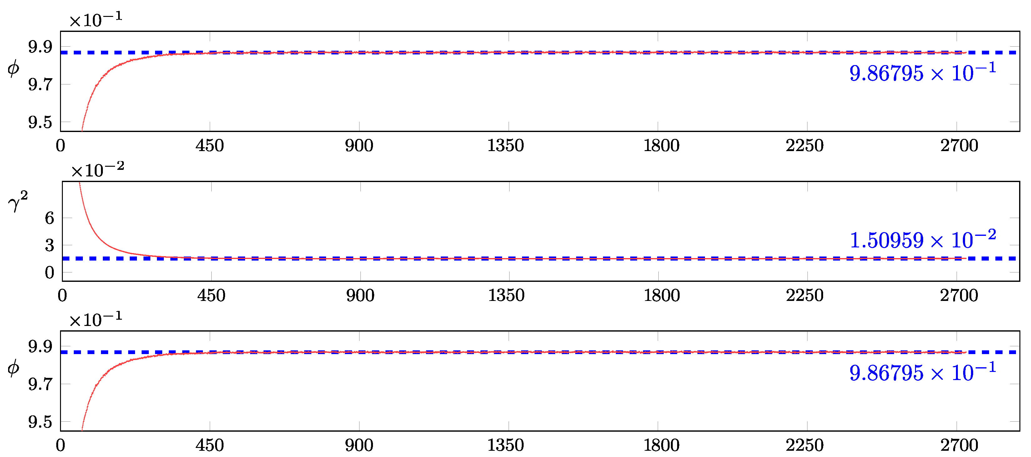
Furthermore, as illuminated in Appendix B.3, the ARSV(1) model is estimated using the offline EM method with a forward-only FFBS algorithm, and the estimates of all of the iterations are shown in Figure 1. We run 2730 offline iterations in total, of which the last 200 iterations have 1250 particles, and the remaining ones use 800 particles. For each parameter estimate, the arithmetic mean of the last 250 iterations is depicted by a blue dashed line, with the mean value marked on the right side, while the red line sketches the estimates across all iterations. As illustrated in Figure 1, the estimates of and quickly converge, while the estimates of fluctuate within a relatively small range around the blue dashed line.
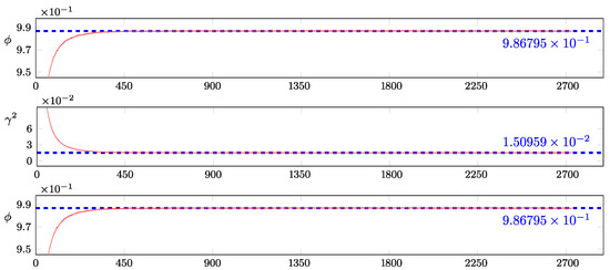
Figure 1.
Particle-based parameter estimates of the ARSV(1) model under the physical measure, Sample A.
Once the parameter estimates of the ARSV(1) model are obtained, its particle-based computations of both the log-likelihood and can be implemented together using particle filtering and smoothing via the bootstrap filter algorithm with particles, as demonstrated in Appendix C.2. The numerical log-likelihood estimation, approximated using Equation (A21) in Appendix C.3, does not require a large number of particles. However, the subsequent particle smoothing does, as it suffers from the degeneracy problem caused by a large observation number ().
Now, let us investigate the distribution of the error terms in the return dynamics. Given the maximum-likelihood parameter estimates and the initial volatility, the volatility at time t () in the GARCH(1, 1) model is fully determined, and thus the error sequence is given by . The ARSV(1) counterpart must be estimated through particle smoothing, as detailed in Appendix C.2. Subsequently, we can obtain the error sequence , in which the denominator (in-sample volatility estimate) is computed using Equation (A15). Both models assume that the return process errors follow the standard normal distribution.
The Q-Q plots versus the assumed standard normal distribution for the error sequences of the two models are shown in Figure 2, and the corresponding normality test results are reported in Table 3, in which the preferred value in each row is underlined. The Q-Q plots indicate that the error sequences of both models have slightly lighter right tails than the standard normal distribution. As for the left tail, the error sequence of the GARCH(1, 1) model is much heavier than a standard normal distribution, while the ARSV(1) counterpart is almost identical to the standard normal distribution. Moreover, considering the result of each normality test whose null hypothesis assumes that the tested sample follows the standard normal distribution, the ARSV(1) model always has a larger p-value. Therefore, when it comes to fitting historical returns, the ARSV(1) model’s normality assumption for the error sequence is more appropriate than that of the GARCH(1, 1) model. This conclusion is in accordance with the findings of Carnero et al. (2004).
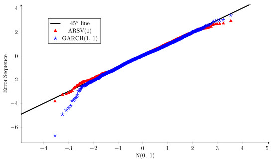
Figure 2.
Q-Q plots: error sequences of GARCH(1, 1) and ARSV(1) models vs. standard normal distribution, Sample A.
Table 3.
Normality tests for the error sequences, Sample A.
As a whole, the ARSV(1) model has a larger likelihood when fitting historical returns and is better for satisfying the assumption that the error sequence in the return process follows a standard normal distribution. Therefore, the ARSV(1) model outperforms the GARCH(1, 1) model in terms of the in-sample comparison under the physical measure.
4.1.2. Out-of-Sample Comparison Under the Physical Measure
The out-of-sample return dataset, Sample B, follow the in-sample dataset without any gap. Therefore, the last in-sample volatility estimate can be directly used to generate the first out-of-sample volatility forecast. This kind of one-step-ahead prediction is natural for the GARCH(1, 1) model since it is exactly how this model works. Given the last in-sample conditional variance estimate and the out-of-sample magnified return series, all of the out-of-sample conditional variances are determined through the specification of the conditional variance in the GARCH(1, 1) model step by step as follows:
where denote the in-sample maximum-likelihood parameter estimates, is the last in-sample conditional variance estimate, T is the size of the in-sample dataset, and is the size of the out-of-sample one. In light of the ARSV(1) model, the out-of-sample volatility forecasts are still particle-based. Fortunately, as demonstrated in Appendix C.4, the one-step-ahead prediction can be connected seamlessly with the particle filtering; that is, the ARSV(1) out-of-sample conditional variance estimate is given by
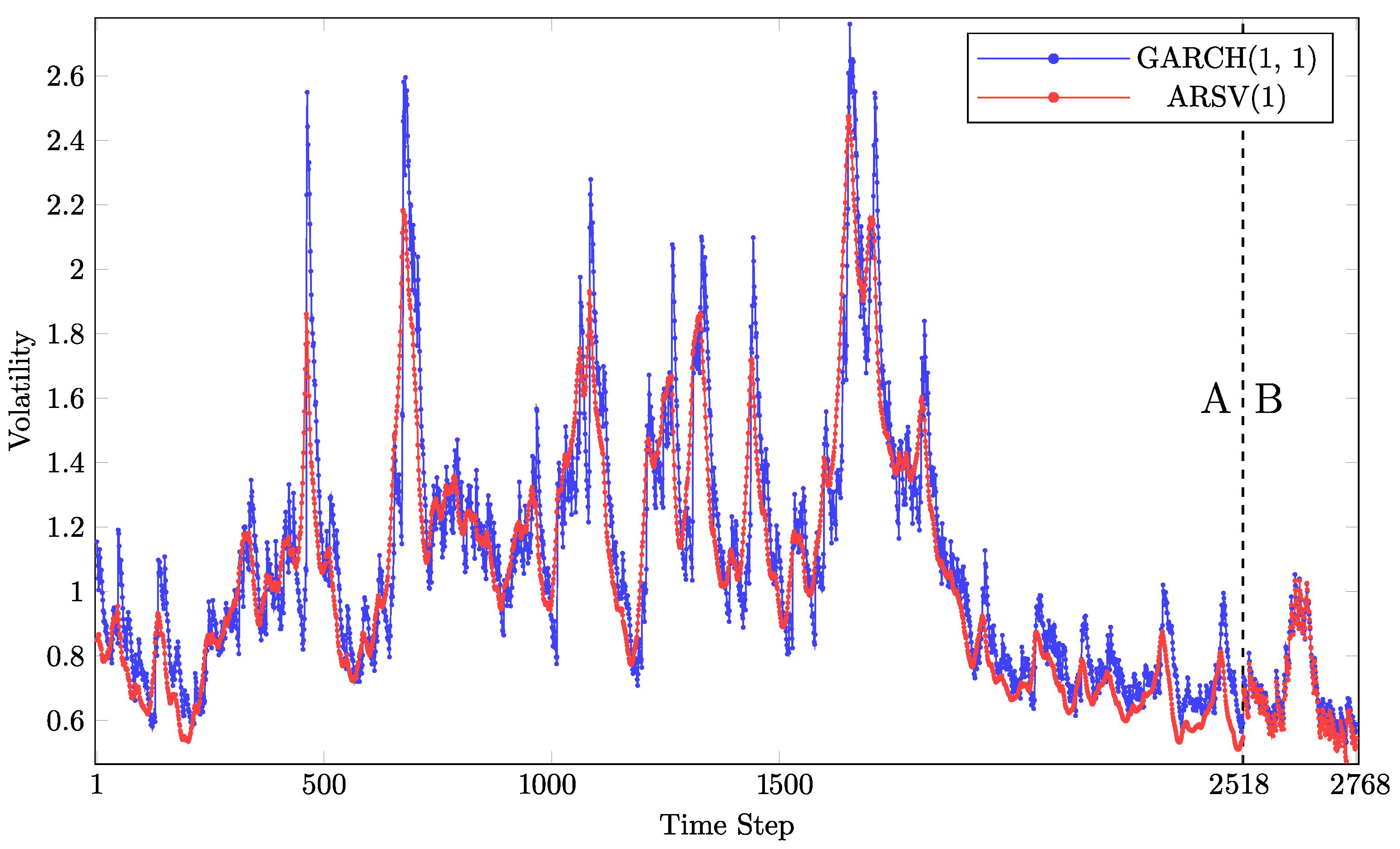
Its parameter estimates are also determined based on the in-sample dataset and stay unchanged for the out-of-sample forecasts. Figure 3 shows both the in-sample and out-of-sample volatility estimates. It illustrates that the two models’ volatility estimates follow similar patterns, though their magnitudes differ.
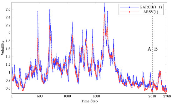
Figure 3.
In-sample (A) and out-of-sample (B) volatility estimates.
The out-of-sample volatility forecast results of the two models are summarized in Table 4, in which the preferred value in each row is underlined. As it shows, the ARSV(1) model has smaller values for the MSE and QLIKE loss functions, so it is also superior to the GARCH(1, 1) model in terms of the out-of-sample volatility forecast under the physical measure.
Table 4.
Out-of-sample volatility forecast results of the GARCH(1, 1) and ARSV(1) models, Sample B.
4.2. Results Under the Risk-Neutral Measure
The S&P 500 Index European call and put options are investigated separately. For each kind of option, we split them into two groups: one expires in about 30 calendar days, and the other expires in about 50 calendar days.
In addition to the GARCH(1, 1) and ARSV(1) models, we investigate the traditional B-S model and the B-S model with implied volatility (BS-IV). Both the traditional BS model and the BS-IV model assume a constant volatility across the time to maturity when pricing options. We set the initial volatility in the traditional B-S model to be the same as the initial volatility in the GARCH(1, 1) and ARSV(1) models. On the other hand, the BS-IV model parameterizes its initial volatility when minimizing the in-sample MSPE as follows:
where is the close price of in-sample Day t; n is the number of in-sample call options; is the constant daily risk-free rate (); and , , and are the time to maturity (in trading days), strike price, and market price of the i-th option, respectively. We want to mention that even though the our in-sample or out-of-sample options are chosen on a single day and expire in about 30 or 50 days, their times to maturity may vary slightly, such as 31 or 33 days. The risk-neutral GARCH(1, 1) and ARSV(1) models for the n in-sample call options at t are estimated as follows:
where the theoretical option prices and are calculated, respectively, using Equations (8) and (16) using the given initial volatility estimate, , along with the identifications (the strike price and time to maturity ) of the i-th option. All three risk-neutral models (BS-IV, GARCH(1, 1), and ARSV(1)) for the put options are estimated similarly.
It is worth noting that the in-sample risk-neutral parameter estimates remain unchanged for the out-of-sample option pricing. Moreover, the initial volatility estimate of the risk-neutral B-S, GARCH(1, 1), and ARSV(1) models comes from the historical daily returns, while it is the only parameter in the BS-IV model. In fact, the in-sample and out-of-sample performances of the B-S model depend entirely on the initial volatility estimates and option selections. Table 5 summarizes the average risk-neutral parameter estimates, with the corresponding standard deviations in the sample in parentheses . The average in-sample and out-of-sample option pricing errors are reported in Table 6 and Table 7, in which the preferred value in each column is underlined, and the corresponding sample standard deviations are included in parentheses .
Table 5.
Average in-sample risk-neutral parameter estimates.
Table 6.
Average in-sample and out-of-sample call option pricing errors with a given initial volatility.
Table 7.
Average in-sample and out-of-sample put option pricing errors with a given initial volatility.
According to Table 5, the risk-neutral parameters of the GARCH(1, 1) and ARSV(1) models are quite different from their physical counterparts. (The return sequence is magnified 100 times. Without this magnification, the previous in GARCH(1, 1) and in ARSV(1) would divide by 100, while the other parameter estimates would remain unchanged.) For example, for the put options in the GARCH(1, 1) model, is less than , while its physical counterpart is close to 1. By contrast, in the ARSV(1) model is much larger than its physical counterpart. The risk-neutral estimates also depend on the kind of option. in the GARCH(1, 1) is such an example. Interestingly, it seems that the put options have larger volatilities, as the corresponding apparently grows. The pricing errors in the traditional B-S model are exacerbated for put options because the initial volatility is always around , with tiny fluctuations.
Furthermore, although estimating the ARSV(1) model is much more complicated than estimating the GARCH(1, 1) model under the physical measure, estimating their risk-neutral versions requires a similar computational burden. The reason for this is that as previously demonstrated, only one process needs to be simulated in the risk-neutral ARSV(1) model.
4.2.1. In-Sample Comparison Under the Risk-Neutral Measure
For the call options, the GARCH(1, 1) model slightly outperforms its three rivals in terms of the average in-sample MSPE and the standard deviation, regardless of the time to maturity. Therefore, the GARCH(1, 1) model fits the observed call option prices better with less dispersion. However, its superiority over the ARSV(1) and BS-IV models is not as clear.
The in-sample performance of the put options is another story. The ARSV(1) model remarkably dominates over the others for both the 30-day and 50-day put options. In addition, the GARCH(1, 1) model also substantially outperforms the BS-IV model.
Furthermore, options with a longer time to maturity tend to have a larger average in-sample MSPE. Not surprisingly, the traditional B-S model is always inferior to the GARCH(1, 1) and BS-IV models regarding the in-sample pricing error. The reason for this is that with the same initial volatility estimate, the B-S model refers to a special case of the GARCH(1, 1) model. On the other hand, the BS-IV model, whose initial volatility is parameterized, is an optimal version of the B-S model with respect to the in-sample MSPE.
4.2.2. Out-of-Sample Comparison Under the Risk-Neutral Measure
As expected, for all models, the out-of-sample average MSPE is larger than its in-sample counterpart. Moreover, the longer the time to maturity is, the harder it becomes to predict the out-of-sample option prices. For call options, the BS-IV model performs better than the others for 30-day options, while the GARCH(1, 1) model is preferred for 50-day options. The out-of-sample call pricing errors are similar across the models, except for the traditional B-S model.
The obvious superiority of the ARSV(1) model over the others within the in-sample put options is kept for the out-of-sample pricing performances. Overall, the ARSV(1) model is indeed preferable when pricing put options. In contrast, put options are less suitable in the GARCH(1, 1) model than call options. This finding is similar to the result of Heston and Nandi (2000).
One thing we need to pay attention to is the initial volatility estimate for each in-sample trading day. Admittedly, we set the initial volatility casually without examining other strategies. Refined initial values will no doubt improve the option pricing performance of both the GARCH(1, 1) and ARSV(1) models. For example, the initial volatility for a risk-neutral model can be estimated using its physical counterpart. On the other hand, the BS-IV model adopts an implied volatility, but it remains inferior to the two models with variant volatilities in most of the scenarios examined. Therefore, dynamic volatility models like the ARSV(1) and GARCH(1, 1) models are more accurate for option pricing than a constant volatility model.
Instead of using historical returns, we can derive the initial volatility directly from the preceding option prices. This adjustment brings about the implied versions of the GARCH(1, 1) and ARSV(1) models, whose pricing performances are explored in the following subsection.
4.3. Risk-Neutral GARCH(1, 1) and ARSV(1) Models Using Implied Volatilities
Rather than setting a relatively casual value, we can also parameterize the initial volatility estimate in the risk-neutral GARCH(1, 1) and ARSV(1) models. For the call options, the implied versions of the two models are estimated by minimizing the in-sample MSPE of the n options as follows:
where the suffix ‘-IV’ or the subscript ‘iv’ stands for the implied version that parameterizes the initial volatility estimate . In addition, and , which denote the theoretical prices of the i-th call option with the risk-neutral GARCH(1, 1) and ARSV(1) models, are calculated using Equation (8) and Equation (16), respectively. The counterparts for put options can be estimated in a similar way. The in-sample and out-of-sample average MSPE of the implied versions of the two risk-neutral models is presented in Table 8, which includes the standard deviations in parentheses .
Table 8.
Average in-sample and out-of-sample option pricing errors of the implied GARCH(1, 1) and ARSV(1) models.
Table 8 shows that parameterizing the initial volatility leads to a smaller average in-sample MSPE for both the risk-neutral GARCH(1, 1) and ARSV(1) models. Most of the corresponding standard deviations also decrease. Such improvements are within our expectations since the original non-implied versions are just special cases of the implied versions when minimizing the in-sample MSPE. However, an extra volatility parameter also brings about more uncertainties in the out-of-sample results. In terms of the average values and standard deviations of the out-of-sample pricing errors, the implied versions of both models are inferior to their original non-implied counterparts that casually set the initial volatility estimates.
One reason for this is that the in-sample nonlinear-least-squares parameter estimators are to some extent sensitive to the input option identifications, such as the spot price and time to maturity, while parameterizing the volatility would further add to such sensitivity. Moreover, it is likely that the implied models will have an abnormal initial volatility estimate; that is, when minimizing the in-sample MSPE, we may obtain an extremely large initial volatility estimate in the implied models. Then, the subsequent out-of-sample prediction error tends to become out of control. In theory, volatility is a positive real number without an upper bound. To avoid abnormal cases, within our implementation, we constrain the daily initial volatility to be less than in our implementation. When the in-sample initial volatility estimate reaches this upper bound, there is a high possibility that the out-of-sample prediction error will be substantially large. By allowing for a smaller upper bound, the out-of-sample results may be better, but this will make the extra volatility parameter less meaningful. Moreover, the upper bound should be connected to the market situation. For example, in a bear market, the upper bound can be relatively larger. How to set a reasonable upper bound for the initial volatility parameter is worth investigating in the future. Overall, for our option samples, the implied versions of the GARCH(1, 1) and ARSV(1) models are not recommended. After all, the out-of-sample prediction error matters more than the in-sample counterpart.
5. Conclusions
This paper conducts a comprehensive comparison of the GARCH(1, 1) and ARSV(1) models under both the physical and risk-neutral measures. Under the physical measure, we investigate their log-likelihoods after fitting the historical returns and test the normality assumption for their error terms in the return process. Moreover, two robust loss functions, MSE and QLIKE, are adopted for a comparison of the one-step-ahead volatility forecasts. The results show that the ARSV(1) model outperforms the GARCH(1, 1) model in both its in-sample fitting and out-of-sample prediction performance under the physical measure.
On the other hand, under the risk-neutral measure, we explore the in-sample and out-of-sample option pricing errors of the two models. We show that only the volatility process in the ARSV(1) model needs to be simulated for option pricing. In addition, we consider both the original and implied versions of the two risk-neutral models. The traditional and implied B-S models are also examined as benchmarks. We find that the performances of the two models are quite similar when pricing call options, while the ARSV(1) model is remarkably superior to the GARCH(1, 1) model for pricing put options. In addition, their implied versions are not robust for out-of-sample option price prediction.
For the non-implied versions of the risk-neutral GARCH(1, 1) and ARSV(1) models, we adopt a causal initial volatility estimate when investigating their in-sample and out-of-sample pricing errors. It is indeed likely that other selections could lead to a better performance. When parameterizing the initial volatility in the implied version, how to set a reasonable upper bound for this parameter is also worth studying. Moreover, instead of the original normal distribution, using the GARCH(1, 1) and ARSV(1) with Leptokurtic distributions, such as Student’s t and exponential distributions, could be explored in the future.
Author Contributions
Conceptualization, T.P. and Y.Z.; methodology, T.P. and Y.Z.; simulation and validation, Y.Z.; investigation, T.P. and Y.Z.; writing—original draft preparation, Y.Z.; writing—review and editing, T.P.; data curation and visualization, Y.Z.; supervision and project administration, T.P. All authors have read and agreed to the published version of the manuscript.
Funding
This research received no external funding.
Data Availability Statement
Data are contained within the article.
Acknowledgments
The authors would like to express their gratitude to reviewers for their careful reading and insightful, constructive comments.
Conflicts of Interest
The authors declare no conflicts of interest.
Appendix A. The Two Forms of the ARSV(1) Model
The first version of the ARSV(1) model is
The second equation can be transformed into the following equation:
where . Let , and we have Therefore, the ARSV(1) model above is transformed as follows:
where . One change we need to pay attention to is that the conditional variance in the former version is denoted by , while it is denoted by in the new one.
Appendix B. A Forward-Only Version of the FFBS Algorithm with the EM Method
Appendix B.1. Forward Filter Backward Smoothing
As shown in Equation (3), the ARSV(1) model belongs to the family of state space models consisting of a transition equation for the state variable (x) and a measurement equation for the observation variable (y). In the ARSV(1) model, the unobservable state variable, , is independent of the states and observations in the past if is given:
If the innovation term in the transition equation is independent of that in the observation equation, we also have
Here, denotes the sequence , follows a prior distribution, is the parameter vector, , and are the transition and measurement equations, respectively. Given n observations, suppose that , is a sequence of functions and denotes the corresponding sequence of additive functionals built from . Then, the smoothed additive functional is defined by
If is in the form of additive functionals, the challenging approximation of can be simplified using a forward-only version of the FFBS algorithm proposed by Del Moral et al. (2010). An auxiliary function is defined by
is generally set to equal 0, and can be obtained recursively as follows:
where is approximated using the forward filtering weighted particles as follows:
Particle filter methods such as bootstrap filter (BF) and Auxiliary Particle Filter (APF) (see Appendix C.1) are feasible in the necessary forward filtering process. Obviously, we have based on Equation (A3). Thus, based on Equations (A4)–(A6), an algorithm for approximating is presented in Algorithm A1.
| Algorithm A1 Algorithm to Approximate the Smoothed Additive Functional |
|
Appendix B.2. The Offline EM Method
When maximizing the particle-based likelihood, techniques such as gradient ascent and EM methods can be adopted in the form of online or offline schemes. The offline scheme means updating the parameter estimates after capturing all of the observations, while the online scheme updates the parameter estimates every time a new observation arrives. Generally, a market dataset is not large enough for the online scheme, so the offline scheme is used in this paper. Moreover, the EM method, if feasible, is preferred to the gradient ascent method because it involves no concerns about the step size problem. The parameter vector at the -th iteration is updated as follows:
where denotes the expectation of the E-step, and is the parameter vector at the l-th iteration. If of a model (e.g., the ARSV(1) model) belongs to the exponential family, the maximizing step in Equation (A7) can simply be finished through a function of sufficient statistics calculated using the forward-only FFBS algorithm as below.
Suppose is the collection of m sufficient statistics that is necessary for the update function. The summary statistic is calculated by
where is in the additive form of Equation (A3). That is why the forward-only FFBS algorithm is feasible for calculating the summary statistics. We first transform into the following form:
where is the sufficient statistics vector, denotes the scalar product, and is the parameter vector. Cappé (2011) shows the maximizing step can be completed as follows:
where is an m-dimensional vector whose h-th element can be derived using Equation (A8) using the forward-only FFBS. Moreover, is the unique solution of .
Appendix B.3. Estimating the ARSV(1) Model Under the Physical Measure
In this paper, we implement the offline EM likelihood optimization method using a forward-only FFBS algorithm to estimate the ARSV(1) model. According to Equation (3), we transform its into the form of Equation (A9) as follows:
We have , , , , . For ease of presentation, let vector stand for . The unique solution to the complete-data maximum-likelihood equation is derived as follows:
and are solved from the first and third equations in the linear system, respectively. Plugging into the second equation, is also solved. Finally, we have , , . Therefore, the unique solution is .
With four sufficient statistics, we have in the offline EM method. The algorithm for estimating the ARSV(1) model under the physical measure is presented in Algorithm A2.
| Algorithm A2 Algorithm to Estimate ARSV(1) under the Physical Measure |
|
T is the number of observations, is the sequence of log daily returns, ItN is the number of iterations, is a four-dimensional axillary vector, , and has been derived. In step 2.2.1, we implement the BF algorithm to obtain weighted filtering particles given a new observation.
Appendix C. Particle Filter and Smoothing
Appendix C.1. Auxiliary Particle Filter
The Auxiliary Particle Filter (APF) algorithm with the given parameter vector is presented in Algorithm A3.
| Algorithm A3 The Auxiliary Particle Filter Algorithm |
|
Appendix C.2. Particle Filtering Together with Smoothing Using a Bootstrap Filter
The particle filtering along with smoothing using bootstrap filter with the given parameter vector is detailed in Algorithm A4.
| Algorithm A4 Particle Filtering Along with Smoothing Using Bootstrap Filter |
|
This algorithm re-samples particles with their ancestors so that the smoothing process is also finished; that is, the re-sampling step at t is conducted for the whole particle path . At each time step , is approximated using the particles with normalized weights as follows:
Therefore, at the final time step T, the joint posterior density can be approximated by
As previously mentioned, this algorithm also solves the smoothing problem. It is straightforward to approximate by marginalizing , as in Equation (A14).
where is the s-th element of the vector (or path) . In addition, the volatility at time s () is approximated by
However, when is very large, only a few of the original particles at time step s will be kept at the final time step. To alleviate this kind of degeneracy problem, we increase the number of particles to .
Appendix C.3. Particle-Based Log-Likelihood Computation
Given the approximated and (), particle filtering provides a numerical solution for the likelihood estimation. Firstly, the marginal likelihood is approximated by
where and are derived using the Bootstrap Filter algorithm as follows:
The simplification from Equation (A18) to Equation (A19) results from the Markovian property of the observation and transition processes in the state space model, including the ARSV(1) model. Within the bootstrap filter algorithm, we generate , while the previous re-sampling step is conducted based on ; then, we have . Consequently, Equation (A19) can be approximated by
As a whole, the particle-based computations of the marginal likelihood and log-likelihood are approximated by
Appendix C.4. Particle-Based One-Step-Ahead Prediction Using the Bootstrap Filter
Under the state space model, the one-step-ahead prediction density is given by
Revisiting the particle filtering along with smoothing algorithm using the bootstrap filter in Appendix C.2, we have
where is the re-sampling index at , and the weighted particles are obtained at time step t. Therefore, the particle-based one-step-ahead prediction using bootstrap filter is summarized in Algorithm A5.
| Algorithm A5 Particle-Based One-Step-Ahead Prediction Using Bootstrap Filter |
|
The size of the out-of-sample dataset is . The first step above is to obtain the weighted particles at the last in-sample step. Since the out-of-sample dataset follows the in-sample counterpart without any gap, the first step in the out-of-sample observations is at . If there is a gap between the in-sample and out-of-sample datasets, the algorithm above needs to be adjusted.
References
- Andersen, Torben G., Tim Bollerslev, Francis X. Diebold, and Paul Labys. 2001. The distribution of realized exchange rate volatility. Journal of the American Statistical Association 96: 42–55. [Google Scholar] [CrossRef]
- Andrieu, Christophe, Arnaud Doucet, and Roman Holenstein. 2010. Particle markov chain monte carlo methods. Journal of the Royal Statistical Society: Series B (Statistical Methodology) 72: 269–342. [Google Scholar] [CrossRef]
- Awartani, Basel M. A., and Valentina Corradi. 2005. Predicting the volatility of the S&P-500 stock index via GARCH models: The role of asymmetries. International Journal of Forecasting 21: 167–83. [Google Scholar]
- Bakshi, Gurdip, and Nikunj Kapadia. 2003. Delta-hedged gains and the negative market volatility risk premium. The Review of Financial Studies 16: 527–66. [Google Scholar] [CrossRef]
- Bakshi, Gurdip, Charles Cao, and Zhiwu Chen. 1997. Empirical performance of alternative option pricing models. The Journal of Finance 52: 2003–49. [Google Scholar] [CrossRef]
- Bollerslev, Tim. 1986. Generalized autoregressive conditional heteroskedasticity. Journal of Econometrics 31: 307–27. [Google Scholar] [CrossRef]
- Cappé, Olivier. 2011. Online EM algorithm for hidden Markov models. Journal of Computational and Graphical Statistics 20: 728–49. [Google Scholar] [CrossRef]
- Carnero, M. Angeles, Daniel Peña, and Esther Ruiz. 2001. Is Stochastic Volatility More Flexible Than GARCH? DES—Working Papers. Statistics and Econometrics. ws010805. Madrid: Universidad Carlos III de Madrid, Departamento de Estadística. [Google Scholar]
- Carnero, M. Angeles, Daniel Peña, and Esther Ruiz. 2004. Persistence and kurtosis in garch and stochastic volatility models. Journal of Financial Econometrics 2: 319–42. [Google Scholar] [CrossRef]
- Christoffersen, Peter, and Kris Jacobs. 2004. Which GARCH Model for Option Valuation? Management Science 50: 1204–21. [Google Scholar] [CrossRef]
- Dahlen, Kai Erik, and Per Bjarte Solibakke. 2012. Scientific stochastic volatility models for the european energy market: Forecasting and extracting conditional volatility. The Journal of Risk Model Validation 6: 17. [Google Scholar] [CrossRef]
- Del Moral, Pierre, Arnaud Doucet, and Sumeetpal Singh. 2010. Forward smoothing using sequential Monte Carlo. arXiv arXiv:1012.5390. [Google Scholar]
- Duan, Jin-Chuan. 1995. The GARCH option pricing model. Mathematical Finance 5: 13–32. [Google Scholar] [CrossRef]
- Engle, Robert F. 1982. Autoregressive conditional heteroscedasticity with estimates of the variance of united kingdom inflation. Econometrica: Journal of the Econometric Society 50: 987–1007. [Google Scholar] [CrossRef]
- Engle, Robert F., and Victor K. Ng. 1993. Measuring and testing the impact of news on volatility. The Journal of Finance 48: 1749–78. [Google Scholar] [CrossRef]
- Heston, Steven L., and Saikat Nandi. 2000. A closed-form GARCH option valuation model. The Review of Financial Studies 13: 585–625. [Google Scholar] [CrossRef]
- Hull, John, and Alan White. 1987. The pricing of options on assets with stochastic volatilities. The Journal of Finance 42: 281–300. [Google Scholar] [CrossRef]
- Kalaylıoğlu, Zeynep I., and Sujit K. Ghosh. 2009. Bayesian unit-root tests for stochastic volatility models. Statistical Methodology 6: 189–201. [Google Scholar] [CrossRef]
- Lehar, Alfred, Martin Scheicher, and Christian Schittenkopf. 2002. GARCH vs. stochastic volatility: Option pricing and risk management. Journal of Banking & Finance 26: 323–45. [Google Scholar]
- Low, Buen Sin, and Shaojun Zhang. 2005. The volatility risk premium embedded in currency options. Journal of Financial and Quantitative Analysis 40: 803–32. [Google Scholar] [CrossRef]
- Malmsten, Hans, and Timo Teräsvirta. 2010. Stylized facts of financial time series and three popular models of volatility. European Journal of pure and applied mathematics 3: 443–77. [Google Scholar]
- Patton, Andrew J. 2011. Volatility forecast comparison using imperfect volatility proxies. Journal of Econometrics 160: 246–56. [Google Scholar] [CrossRef]
- Skoglund, Jimmy, Donald Erdman, and Wei Chen. 2010. The performance of value-at-risk models during the crisis. The Journal of Risk Model Validation 4: 3. [Google Scholar] [CrossRef]
- Taylor, Stephen. 1982. Financial returns modelled by the product of two stochastic processes, a study of daily sugar prices 1961–79. Time Series Analysis: Theory and Practice 1: 203–26. [Google Scholar]
- Yu, Jun. 2002. Forecasting volatility in the New Zealand stock market. Applied Financial Economics 12: 193–202. [Google Scholar] [CrossRef]

Disclaimer/Publisher’s Note: The statements, opinions and data contained in all publications are solely those of the individual author(s) and contributor(s) and not of MDPI and/or the editor(s). MDPI and/or the editor(s) disclaim responsibility for any injury to people or property resulting from any ideas, methods, instructions or products referred to in the content. |
© 2025 by the authors. Licensee MDPI, Basel, Switzerland. This article is an open access article distributed under the terms and conditions of the Creative Commons Attribution (CC BY) license (https://creativecommons.org/licenses/by/4.0/).