Article

An Integrated Risk Management Methodology for Deposits and Loans

by
Gregory R. Hackworth
1,
Weidong Tian
2,* and
Michael R. Vandenberg
1
1
Bulls-Eye Solutions, LLC, Charlotte, NC 26173, USA
2
Belk College of Business, University of North Carolina at Charlotte, Charlotte, NC 28223, USA
*
Author to whom correspondence should be addressed.
Risks 2025, 13(3), 52; https://doi.org/10.3390/risks13030052
Submission received: 29 December 2024 / Revised: 27 February 2025 / Accepted: 3 March 2025 / Published: 13 March 2025
(This article belongs to the Special Issue Valuation Risk and Asset Pricing)

Abstract

:
This paper presents an integrated risk management methodology for measuring and managing the economics, risks, and financial resources/constraints related to deposits and loans in a commercial bank. Within a comprehensive and integrated framework, we develop valuation and risk models for all financial products on the bank’s balance sheet. Our proposed methodology aligns with regulatory requirements while offering a practical implementation. Unlike traditional industry practices, which often rely on fragmented and siloed risk management solutions, our approach integrates risk modeling across all aspects of the bank’s balance sheet. This new perspective provides a more accurate and consistent assessment of financial risks, improving the bank’s ability to navigate regulatory and economic challenges.
JEL Classification:
G11; G12; G13

1. Introduction

Fluctuations in the interest rate environment can significantly affect the value of deposit and mortgage loan products for a commercial bank, resulting in substantial risk management challenges and considerations. The events of 2023 underscore the critical need for robust risk management systems. The collapses of Silicon Valley Bank (SVB), Signature Bank (SBNY), and First Republic Bank (FRB), as well as the bank runs experienced by Silicon Valley Bank and Silvergate Bank (SICP), revealed systemic failures stemming from inadequate asset and liability mismatch management, concentration risk in volatile sectors, and insufficient regulatory supervision (see Diamond and Dybvig 1983; Barr 2023). The inability to manage interest rate risk effectively was a key factor in these failures, alongside broader governance and market concentration issues.1
From a modern risk management perspective, it is essential for a commercial bank to develop business strategies that integrate both deposits and mortgage loans to effectively manage financial resources (capital, liquidity, etc.) and risks to those same resources. The classical duration-based approach to asset–liability management is inadequate for addressing interest rate risk. In particular, the deterministic interest rate assumption commonly used in duration-based models (see Fisher and Weil 1971) is widely considered unrealistic from both theoretical and empirical perspectives. Consequently, financial modelers and risk managers often rely on term structure models of interest rates to calibrate prevailing yield curves and market-available data within an arbitrage-free framework (see, for instance, Andersen and Piterbarg 2010).
However, valuation and risk management models for deposits and mortgages are often developed independently. On the one hand, equilibrium and no-arbitrage approaches for deposit account have been widely explored. Notable examples include the works of Hutchison and Pennacchi (1996), Jarrow and Deventer (1998), Janosi et al. (1999), and Sheehan (2013), which also incorporate behavior into their frameworks. On the other hand, econometric and no-arbitrage models are predominantly used for mortgage loans and related mortgage-backed securities (MBS). For instance, see Stanton (1995), Chernov et al. (2018), and references therein.
Moreover, the assumptions in these valuation and risk models, as found in the academic literature and market practice (see, for instance, Janosi et al. 1999; Chernov et al. 2018; Moulin 2020; Wyle 2014), are not always consistent and may even contradict one other due to the myriad of risk factors and the complexity of financial products. For a commercial bank, it is essential to establish consistent and economically sound assumptions across all products on the balance sheet. Furthermore, given the significance of scenario analysis and stress testing, an integrated framework capable of effectively simulating future scenarios for all balance sheet products and assessing their impact on financial resources is crucial in modern risk management.
We aim to present such a comprehensive and consistent risk management framework for asset and liability management. In this integrated risk management methodology, we identify fundamental factors that impact the value of assets and liabilities and develop a model to measure the economic impact of changes in these factors. We first develop a combination of equilibrium and behavioral models for the deposit accounts in a commercial bank. Building on the fundamental factors and scenarios, we derive the deposit rates, deposit accounts, and the aggregate balance across cohort at the bank level. In this regard, our model differs from the dynamic deposit model in Drechsler et al. (2021), where deposit franchises grant banks market power, allowing them to borrow at rates that are both low and insensitive to market interest rates. Since Drechsler et al. (2021) does not account for the liability side, they instead consider operating costs, which are also insensitive to interest rates. Therefore, Drechsler et al. (2021) argue that bank profits remain stable even during significant interest rate fluctuations.
For mortgage loans, we adopt a methodology comparable to that used for deposit products, extending it to incorporate fundamental factor scenarios while integrating both no-arbitrage and behavioral aspects within the valuation model. Additionally, we develop a behavior-based loan demand model as part of this framework. Our methodology introduces several key innovations: (1) ensuring consistent assumptions across assets and liabilities; (2) employing economically sound (equilibrium or no-arbitrage) valuation and risk models for all products; and (3) robust implementations and scenario-driving techniques for risk management. These innovations allow us to derive metrics such as the economic value of equity (EVE), offering a comprehensive understanding of risk and enhancing overall risk management practices. Chernov et al. (2018) develop a no-arbitrage model for valuing mortgage-backed securities using a macroeconomic-driven prepayment function. While our mortgage loan model shares similar features, our prepayment specification can incorporate additional behavioral variables. More importantly, we consider the bank’s funding efficiency and optimization by integrating short-term deposits alongside mortgage loans, using the same macroeconomic factors. In contrast, Chernov et al. (2018) focus solely on the mortgage side.
The structure of this paper is as follows. In Section 2, we present a motivating example to illustrate the concept of an integrated risk management system. This is followed by an in-depth exploration of the deposit side in Section 3 and the mortgage loans side in Section 4. Section 5 focuses on the EVE and various risk measures. Finally, in Section 6, we offer our concluding remarks. For brevity, additional technical details are provided in Appendix A and Appendix B.

2. A Motivated Example

To explain our methodology, we begin with a simple example of asset and liability structure. Consider a commercial bank with a deposit account and a single class of mortgage loan. On the liability side, the bank pays the depositor β R , where β is a constant between 0 and 1, and R represents the interest rate. The initial deposit amount is denoted as D 0 , and we assume a constant decay rate α of the deposit amount. On the asset side, the mortgage borrower pays the bank a fixed mortgage amount c to the bank, with prepayment occurring at a constant hazard rate γ . The key assumption in this setup is that the yield curve remains flat. This assumption facilitates a direct comparison with the classical duration–convexity approach for addressing interest rate risk in, for instance, Fisher and Weil (1971).
We now value both asset and liability for the bank. At time 0, with the interest rate R = R 0 , the asset value is given by
A 0 = c 0 e ( R 0 + γ ) t d t = c R 0 + γ .
The modified duration and the convexity of the asset are given by2
D A ( R ) = A ( R ) A ( R ) = 1 R + γ , C A ( R ) = A ( R ) A ( R ) = 2 ( R + γ ) 2 .
On the liability side, the value of the deposit franchise is
L 0 = 0 e ( R 0 + α ) β R 0 D 0 d t + 0 e ( R 0 + α ) t D 0 d t = β R 0 D 0 + D 0 R 0 + α .
Accordingly, the modified duration and the convexity of the liability are given by
D L ( R ) = 1 α β R ( R + α ) , C L ( R ) = 2 ( 1 α β ) ( 1 + β R ) ( R + α ) 2 .
The EVE is written as
E ( R ) = A ( R ) L ( R ) = c R + γ β R D 0 + D 0 R + α ,
and we assume that A 0 > L 0 , as E 0 = A 0 L 0 denotes the equity funding. We can impose capital requirement conditions, but those conditions do not influence our main conclusions here. The interest rate risk for the bank is essential, as it impacts both liability and asset.
We first consider the classical duration–convexity approach. Assuming a constant beta and letting
D A ( R ) = D L ( R ) ,
we solve this equation to derive
β ( R ) = γ α R 2 + 2 α R + α γ ,
which is a decreasing function of the short rate, depending on the deposit market and the mortgage loan information. However, this beta becomes negative when γ < α . Moreover, Equation (7) indicates that the beta is time-varying, which depends on the interest rate R.
Alternatively, we can solve the first-order derivative matching equation, A ( R ) = L ( R ) , which reduces to
β ( R ) R R + α + β ( R ) α 1 ( R + α ) 2 = c D 0 1 ( R + γ ) 2 .
Solving this ODE yields
β ( R ) = c D 0 R + α R ( R + γ ) 1 R + α + β 0 R + α R
where β 0 is a constant determined by A ( R 0 ) L ( R 0 ) = E 0 . This implies that the beta depends on the EVE, E 0 , in addition to the deposit and mortgage loan structure. This choice of beta can exhibit various behaviors—decreasing, increasing, or hump-shaped—depending on the market structure. Notably, with this time-varying deposit beta, the EVE remains constant regardless of changes in the interest rate. Figure 1 illustrates the distinct effects of a constant versus a time-varying deposit beta. Specifically, with a time-varying deposit beta, the asset consistently exceeds the liability, demonstrating its effectiveness in managing interest rate risk.
While the asset–liability example provided above is simplified and relies on several strong market assumptions, it effectively conveys key insights. This highlights the critical importance of considering both asset and liability components, alongside the EVE, within a unified and consistent framework for managing interest rate risks. This approach is not only feasible but also essential for developing a robust risk management system that comprehensively addresses the dynamic interplay between assets and liabilities.
In our integrated risk management methodology for the deposits and loans, we begin with a no-arbitrage model of interest rates and fundamental economic factors (details provided in Appendix B). The scenarios derived from these interest rates and fundamental factors simultaneously impact both assets and liabilities. We then analyze behavioral models for depositors and mortgage customers (Section 3 and Section 4). For the deposit component, we construct equilibrium models of the deposit rate and deposit demand (Section 3) in each type of deposit account. This equilibrium model contains both no-arbitrage and behavioral natures of pricing. We further construct no-arbitrage valuation models of mortgage loan and mortgage-backed securities (Section 4). This framework allows us to derive the EVE and to report risk measures (Section 6). The outputs also include scenarios of asset and liability cash flow (Section 3 and Section 4).
Figure 2 summarizes the structure of the risk management methodology. By employing this unified and consistent framework, the bank can conduct scenario analysis, stress testing, and Comprehensive Capital Analysis and Review (CCAR), along with meeting various regulatory and internal risk management requirements. Additionally, the methodology empowers the bank to design effective business strategies in the deposit and loan markets, optimize equity value, and minimize risks.

3. Deposits

Non-maturing financial products, such as deposits, present many challenges in predicting cash flows and interest rates. Customers can open or withdraw their deposits at any time, creating uncertainty about the timing of deposit maturities. While some deposits remain with the bank for extended periods, others are short-lived. Moreover, banks have the flexibility to set the interest rates that they offer, competing with other institutions on rates and services. As a result, the deposit rate and the total deposit balance are influenced by customer behavior, the bank’s strategies and management decisions, market conditions, and the broader economic environment.
This section introduces a deposit model to elucidate the interactions between depositors and banks. While we focus on a single bank and a cohort of depositors, we can easily extend this methodology to encompass multiple banks simultaneously, as demonstrated in Hackworth et al. (2024). Depositors within this framework possess the flexibility to allocate their funds within the deposit market, allowing for movement both into and out of the market and between different deposit accounts. The bank optimally sets the deposit rates to maximize the profit of the deposit business. The model captures the dynamic nature of deposits, where funds can flow in and out of the deposit market, and depositors can switch between various account options. The analysis begins with depositor behavior, proceeds to the determination of equilibrium, and concludes with an examination of the deposit franchise valuation problem.

3.1. Behavior Segment

Banks offer various deposit accounts, such as demand deposits, time or savings deposits, fixed or floating rate deposits, and certificates of deposit (CD). On the customer side, there are wholesale and retail depositors. These depositors differ in various aspects, such as life stage, wealth level, behavior, relationship with the bank, financial knowledge, and other demographic factors. These factors collectively influence how depositors manage and interact with their funds.
Given these characteristics of the deposit market from both the supply and demand side, we divide the deposit into segments indexed by i = 1 , 2 , , N . There is a deposit franchise for each segment for a commercial bank. To keep things simple, we assume there is one type of deposit for each segment, and the maturity of the deposit is represented by a random maturity τ i . We assume that each τ i is a stopping time in the filtered probability space ( Ω , ( F t ) , P ) . The distribution of τ i represents the depositor’s behavior in segment i, which can be estimated with a large historical data set.
Several examples of the random maturity τ i are as follows:
  • In a bank-run situation where customers withdraw their deposits, we have P ( τ i = 0 ) = 1 .
  • For deposit with a constant maturity T, P ( τ i = T ) = 1 . As an example, T = 4 months represents short-term liabilities in the form of deposits;
  • When deposit withdrawal follows a geometric distribution, P ( τ i = t ) = α i ( 1 α i ) t 1 , with 0 < α i < 1 . Here, α i represents the probability of exiting the deposit account each period. For instance, an average maturity of 4 months corresponds to a decay rate of α i = 0.25 ;
  • Alternatively, if τ i has a Poisson distribution with parameter λ i , the probability is given by P ( τ i = t ) = e λ i ( λ i ) t t ! . While the average maturity remains the same as the previous example when λ i = α i , the decay rate in each period differs for both distributions of τ i .
The cumulative distribution function of τ i is denoted by F i ( · ) . When a new depositor enters the segment i, we view the new one as the same as the existing one. Given the maturity τ i at time 0, the conditional probability is given by
P ( τ i k | τ i > t ) = F ( k ) F ( t ) 1 F ( t ) ;
In particular,
α i ( t ) P ( τ i = t + 1 | τ i > t ) = F ( t + 1 ) F ( t ) 1 F ( t ) .
This conditional density at time t represents the deposit decay rate in the period from t to t + 1 from the time t perspective. In a stochastic hazard-rate approach, the decay rate between t and t + 1 can depend on the prevailing market information. This approach is further elaborated in Section 4, where we apply it to both the prepayment model and the credit model.

3.2. An Equilibrium Model

In each period, the bank pays the deposit rate. The deposit rate for this segment i at time t is denoted as r i d ( t ) . Let D i ( t ) = ω i ( t ) D ( t ) , where D ( t ) denotes the total (aggregate) deposit balance of the bank and 0 < ω i ( t ) < 1 . In our setting, ω i ( t ) is predetermined up to time t for the following reasons. First, the bank cannot fully and directly determine the balance in each segment but can do so indirectly and partly through the deposit rate. Second, we can calculate ω i ( t ) through regression to r ( t ) or other observable variables at time t. Third, the proportional ω i ( t ) depends on external exogenous behavior factors. This model’s key insight is determining the total balance D ( t ) in equilibrium. Once D ( t ) is established, the segment balance D i ( t ) and the new equilibrium balance can also be determined. Additionally, the deposit rate is calculated in equilibrium. In Hackworth et al. (2024), equilibrium considerations include market share determination, which can be directly applied to the current situation, allowing for a consistent characterization of equilibrium dynamics.
For each segment i, the bank solves the optimization problem (Hutschison 1995; Hutchison and Pennacchi 1996):
max r i d ( t ) r ( t ) r i d ( t ) c i ( t ) ω i ( t ) D ( t )
where c i ( t ) = ζ i + ( 1 ρ i ) r ( t ) denotes the cost, in which 1 ρ i is the deposit required reserve ratio and ζ i the fixed cost.
The bank’s deposit business plan is modeled by the following specification of the aggregate balance.
D ( t ) = e μ t k r ( t ) + i = 1 N k i r i d ( t ) + η ( t )
where μ denotes the growth rater of new balance, while the parameters k and k i represent the coefficients to the interest rate and each deposit rate to the balance. We assume each to be k > 0 , k i > 0 to capture the positive relationship between deposit rate and demand. The last term, η ( t ) , includes other external variables affecting the balance. For example, these could be factors like financial or economic crises, sentiment indices, or other economic variables observed or estimated at time t. However, there is no deposit rate r i d ( t ) in the term η ( t ) .

3.3. Deposit Rate and Balance in Equilibrium

We present the equilibrium and leave the technical details into Appendix A and Appendix B.
First, Equation (13) has an intuitive expression in equilibrium as follows. There exists a positive number l such that
D ( t ) = e μ t k r ( t ) + l r ^ d ( t ) + η ( t ) ,
where r ^ d ( t ) = i = 1 N ω i ( t ) r i d ( t ) is the average deposit rate across different types of deposit. Moreover, the weight in the average deposit rate is the same as the weight of the deposit demand to the total deposit balance. The intuition behind this relationship is straightforward. A high contribution of the deposit rate for one type of deposit account to the total balance also increases the balance in this account. Therefore, the aggregate balance depends on both the interest rate and the aggregate deposit rate. The intuition is that each deposit account contributes consistently to the overall balance of the bank. While varying deposit rats across banks might influence the distribution of deposit, a bank primarily focuses on maximizing its total deposit balance. In other words, the deposit rates across different deposit accounts are not combative with each other.3 The parameter l represents the effect of the aggregate deposit rate on the total balance of an individual commercial bank.
Second, the total balance in equilibrium is given by
D ( t ) = e μ t b l r ( t ) + η ( t ) N + 1 l N + 1 i = 1 N ω i ( t ) ζ i ,
where
b = 1 N + 1 1 + k l i ω i ( t ) ( 1 ρ i ) .
In addition to the growth rate, three components determine the aggregate balance at time t. The first term represents the contribution of the short rate. The second term denotes the contribution of other exogenous variables on the balance, and the last term denotes the total cost incurred in the deposit business.
To understand the equilibrium, it is helpful to examine the effect of the parameter l on the aggregate balance. For simplicity, from now on, we assume that l is time-independent and ρ i = 1 so we can focus only on fixed costs for the deposit service. The higher the value of the parameter l, the higher the average cost endured by the bank in the last term of Equation (15). The value of the parameter b also decreases, and the effect of the short rate decreases to the total balance. The total balance declines as the aggregate deposit rate increases, even when the interest rate remains constant. Conversely, when the value of the parameter l decreases, the value of the parameter b increases, leading to an increase in the total balance, assuming that the interest rate remains unchanged. In the limit case where l = 0 , there is no relationship between the deposit rates and the aggregate balance, and, as a result, the interest rate has no effect on the balance in equilibrium.
Moreover, Equation (16) highlights the economic interpretation of the parameter b in terms of the sensitive parameters k and k i , as well as other parameters { ω i ( t ) , ζ i , i = 1 , , N } . Nevertheless, the value of this parameter b is not arbitrary. For instance, if each ω i ( t ) is independent of the short rate r ( t ) and each ρ i = 1 , then the parameter b satisfies 0 < b < 1 N .
Third, the deposit rate r i d ( t ) for each segment is given by
r i d ( t ) = 1 b ω i ( t ) r ( t ) η ( t ) ( N + 1 ) l ω i ζ i + i = 1 N ζ i ω i ( t ) ( N + 1 ) ω i ( t ) .
By Equation (17), the interest rate affects the deposit rate, and the deposit-beta is given by:
β i = 1 b ω i ( t ) .
Since the total weight must be one, we obtain an interpretation of the parameter b in terms of all deposit rate betas:
i = 1 N 1 1 β i = 1 b .
Remark 1.
Drechsler et al. (2021) highlight that deposit rates are often “sticky” and do not change proportionally with market rates, leading to a mismatch when using static duration models. Equation (17) is consistent with the empirical findings in Drechsler et al. (2021) regarding the effect of the market rates on the deposit rate.
We next investigate the interest rate risk in each deposit in equilibrium. By Equations (13) and (17), we obtain
D ( t ) r ( t ) = e μ t b l l N + 1 i = 1 N ζ i ω i ( t ) r ( t ) .
As shown in Equation (20), the effect of the interest rate on the deposit beta depends on all marginal effects, ω i ( t ) r ( t ) , i = 1 , , N . This model is different from some models of the deposit beta in terms of the interest rate directly.4 The crucial insight in our model is that the interest rate risk in all deposit accounts together affects the deposit account. This justifies an equilibrium model even for one individual bank.
Similarly, we can analyze the first-order and second-order effects of the interest rate on the deposit beta. For example, β i ( t ) r ( t ) = b ω i ( t ) 2 ω i ( t ) r ( t ) , and the deposit convexity is given by
2 β i ( t ) r ( t ) 2 = b ω i ( t ) 2 2 ω i ( t ) r ( t ) 2 2 ω i ( t ) ω i ( t ) r ( t ) 2 .
In equilibrium, we derive the aggregate deposit rate as follows:
r ^ d ( t ) = ( 1 b N ) r ( t ) N ( N + 1 ) l η ( t ) 1 N + 1 i ζ i ω i ( t )
Consequently, the aggregate deposit beta is given by
r ^ d ( t ) r ( t ) = 1 b N 1 N + 1 i ζ i ω i ( t ) r ( t ) .
Again, the aggregate deposit beta relies on all marginal effects ω i ( t ) r ( t ) , i = 1 , , N .
Finally, we examine the effect of the interest rate on the deposit balance in each segment. Since D i ( t ) = ω i ( t ) D ( t ) , we obtain
D i ( t ) r ( t ) = ω i ( t ) e μ t ( b l ) + D ( t ) ω i ( t ) r ( t ) .
In contrast to the deposit beta, the effect of the interest rate on the balance—referred to as the balance beta, D i ( t ) r ( t ) —can be positive or negative. There is at least one segment whose deposit beta and demand positively depend on the interest rate. However, when the short rate has a negative effect on the share ω i , the deposit beta negatively depends on the short rate, and the demand beta can be either positive or negative. On the bank level, however, the average balance beta remains positive. In our deposit model, the deposit beta is time-dependent. The deposit beta and demand maintain a proportional relationship with the interest rate through analyzing the market share ω i ( t ) .
Thus far, our analysis has operated under the assumption that η ( t ) remains unaffected by the interest rate’s term structure. To broaden our perspective, we now incorporate the entire term structure into our equilibrium framework. For example, we can incorporate the slope and curvature of the interest rate occurred in the term η ( t ) , since r ( t ) only captures the “level” of the interest rate. Let η ( t ) = s 1 ( r ( t ) r ( t 1 ) ) + η ¯ ( t ) , where η ¯ ( t ) denotes other variables besides the term structure; then,
r i d ( t ) = β i r ( t ) s 1 ( N + 1 ) l ω i ( t ) ( r ( t ) r ( t 1 ) ) ζ i + i ω i ζ i ( N + 1 ) ω i .
In this way, the deposit rate depends on both the level and the slope of the interest rate curve.

3.4. Deposit Valuation

We discuss the valuation of the deposit franchise at each segment i. By calculation, the cash flow at time t for segment i is
( r ( t ) r i d ( t ) c i ) D i ( t ) = b r ( t ) + η ( t ) ( N + 1 ) l ω i ( t ) ζ i N + 1 D ( t ) ,
where D ( t ) is given in (15). Therefore, each deposit segment is a sequence of floating-rate cash flow. In our model, the difference between these segment is characterized by the distribution of the maturity of each segment, a behavior characterization.
The no-arbitrage price of the deposit franchise at time 0 is given by
V i ( 0 ) = E Q t = 0 e t r ( t ) b r ( t ) + η ( t ) ( N + 1 ) l ω i ( t ) ζ i N + 1 D ( t ) Q ( τ i = t ) ,
where Q ( τ i = t ) is the risk-neutral probability of the depositor exiting, and E Q [ · ] denotes the expectation operator under the risk-neutral probability measure. We assume a well-diversified group of depositors and that the exiting premium can be hedged. In a general stochastic model of the exiting probability, we can add the premium term as in the mortgage model, which we explain in the next section.
The value process of the deposit franchise is given by
V i ( t ) = E t Q s = t e ( s t ) r ( s ) b r ( s ) + η ( s ) ( N + 1 ) l ω i ( s ) ζ i N + 1 D ( s ) Q ( τ i = s ) | τ i > t .
Its continuous version is given by
V i ( t ) = E t Q t e x p t s r ( u ) d u b r ( s ) + η ( s ) ( N + 1 ) l ω i ( s ) ζ i N + 1 D ( s ) Q ( τ i = s ) | τ i > t .
Finally, the duration of each deposit is the duration of the corresponding float-rate security. Namely,
D u r a t i o n i = E Q 0 e x p 0 t r ( u ) d u b r ( t ) + η ( t ) ( N + 1 ) l ω i ( t ) ζ i N + 1 t D ( t ) Q ( τ i = t ) d t V i ( 0 ) .
In our framework, the interest rate and other pertinent variables denoted as r ( t ) , η ( t ) are exogenously determined. Therefore, we have the flexibility to integrate any Heath–Jarrow–Morton-type model for interest rates, along with macroeconomic models, into our valuation methodology; refer to Appendix B for details. We are capable of deriving analytical valuation expressions for various interest rate models, including Gaussian interest rate models. If there is a concern regarding negative interest rates within the framework of a Gaussian model, quadratic-type interest rate models, as discussed in the works of Boyle and Tian (1999) and Ahn et al. (2002), are viable alternatives in the framework. Analytical expressions for such models are readily accessible for implementation within our valuation framework.

3.5. Run-Off Balance

The number α i ( t ) = P ( τ i = t + 1 | τ i > t ) represents the decay rate for the segment i in the time period from t to t + 1 . This means that α i ( t ) D i ( t ) is the exiting balance. Therefore, the new balance in this time period is D i + 1 ( t ) ( 1 α i ( t ) ) D i ( t ) . The difference between the entry balance and the exiting balance, E n t r y i , t E x i t i t , becomes D i + 1 ( t ) ( 1 α i ( t ) ) D i ( t ) α i ( t ) D i ( t ) = D i ( t + 1 ) D i ( t ) .
On the bank aggregate level, i α i ω i ( t ) is the decay rate of the total balance in the period from t to t + 1 . Unless each ω i ( t ) is independent from the market situation, there exists at least a positive one and a negative value of ω i ( t ) r ( t ) . Therefore, the average decay rate is, in general, stochastic, depending on the market situation. Since the difference between total new and exiting balance is D ( t + 1 ) D ( t ) , we obtain
E n t r y i , t E x i t i t D ( t + 1 ) D ( t ) = ω i ( t + 1 ) D ( t + 1 ) ω i ( t ) D ( t ) D ( t + 1 ) D ( t ) .
This ratio measures the stability of demand in segment i. Specifically, a small value of the ratio indicates low turnover in the deposit account, while a large value suggests high depositor turnover within this segment.
It is possible that the depositor exits from the segment i but still keeps it in the bank. Let p i j ( t ) be the probability of depositor in segment i moving to segment j. Let P ( t ) be the transformation matrix, ( p i j ( t ) ) . We can estimate the forever exiting probability from the bank with the historical data and consumer behaviors. For simplicity, we assume the depositor stays in the bank forever. Then, we obtain
α i ( t ) D i ( t ) = j = 1 N p i j ( t ) D j ( t ) .
Alternatively,
j = 1 N p j i ( t ) ω j ( t ) = α i ( t ) ω i ( t ) .
For a certain specification of the matrix P, we can explicitly express P using the weight vector. Conversely, if the transformation matrix P is estimated first, the weight vector ( ω 1 ( t ) , , ω N ( t ) ) can be derived. For example, it corresponds to an eigenvector of the matrix P d i a g ( α 1 , , α N ) , associated with an eigenvalue 0.

4. Mortgage Loans

In this section, we develop a mortgage loan modeling system tailored for commercial banks. We adopt the same framework as in the previous section, employing fundamental models of the interest rate denoted as r ( t ) and economic or other exogenous variables denoted as η ( t ) . Additionally, we apply a similar methodology used for deposit accounts to construct models for mortgages and loans.
Building on deposit dynamics, we now model loans with consistent factors. Our approach begins by examining the segment and behavior of mortgage customers. Next, we introduce the prepayment model, followed by the loan demand model and its corresponding valuation model. Additionally, we incorporate a credit risk model to evaluate the risks associated with loan products. Importantly, this credit model can also be extended to address uninsured deposits and the risk of bank runs. Finally, we note that the stochastic prepayment model can be integrated into deposit models to account for the stochastic decay rate.

4.1. Segment

Similar to analyzing the deposit portfolio, it is essential to examine the loan portfolio by considering various factors. These include loan-specific information such as loan amount, interest rate, loan term, type of loan, and history of previous loans or defaults, as well as borrower-specific details such as credit score, employment status, income level, number of dependents, marital status, age, alertness, knowledge, and educational qualifications.
To facilitate analysis, mortgages can be segmented based on borrower characteristics or, alternatively, by mortgage characteristics. The latter approach is particularly suitable for managing mortgage-backed securities or large portfolios of mortgage loans. For this reason, we adopt the second approach to segment mortgages in our analysis.

4.2. Prepayment Model

We start with a single mortgage of a fixed mortgage rate m > 0 with a capital equal to K. Then, the mortgage amount c is determined by
K = c 0 T e m t d t ,
and, thus,
c = K m 1 e x p ( m T ) .
The principal balance at time t < T , denoted by I t , satisfies
d I t = ( m I t c ) d t , I 0 = K .
From the bank’s perspective, the risk is that the borrower exercises his/her prepayment option at time t, when the interest rate r ( t ) becomes low. This means that the bank receives I t instead of the future stream of payment c. Let τ be the prepayment time. Therefore, the value of the mortgage is given by
V 0 = E Q e 0 τ r ( t ) d s I τ
In a rational no-arbitrage approach, we can study the optimal stopping time τ * by viewing it as an American-type derivative—see, for instance, Detemple and Tian (2002). However, the optimal behavior of the prepayment is not consistent with the market behaviors.
Alternatively, we can define
Q ( τ t ) = 1 e x p 0 t π ( s ) d s
for a hazard rate π ( · ) . Similar to the decay rate of a deposit account before, we take a deterministic hazard rate assumption. Then, we obtain
V 0 = E Q 0 e 0 s ( r ( t ) + π ( t ) ) d t I s d s
For instance, for certain exogenous variable η ( t ) , the hazard rate can be chosen as π ( t | η t ) = λ + τ * η t —see, for instance, Stanton (1995). A linear specification of the hazard rate π ( · | η ) leads to analytical valuation expression as shown in Appendix B. For other mortgage loan pricing models, refer to Karpishpan et al. (2010) and Fermanian (2013).
The stochastic hazard-rate approach for the prepayment time is conceptually similar to mortgage-backed securities (MBS) valuation. So, we explain only the MBS in the subsequent discussion. For the prepayment risk in the MBS, we focus on the notional balance percentage in the pool, whereas we consider the distribution of the prepayment time for a single mortgage.
Specifically, let N t denote the remaining notional balance (as the percentage) of the underlying mortgage pool at time t. We write
N t = e x p 0 t p s d s ,
then, N t I t is the remaining principal balance of the underlying pool. Then, the value of the MBS at time 0 is
V 0 = E Q 0 T e x p 0 t ( r ( s ) + h ( s ) ) d s N t ( c + p t I t ) d t
where h ( s ) denotes a credit or liquidity spread that will be explained shortly. In its discrete-time expression,
V 0 = E Q k = 1 K P ( 0 , t k ) j = 1 k ( 1 p ( t j ) ) c + p ( t k ) I ( t k )
for s sequence of mortgage payment times t 1 , , t K = T . Here, the stochastic model is to present a stochastic process of p t , or π t .
Our system constructs a behavioral and statistical model of the parameter p t , often using a linear regression framework. As shown in Appendix B, a linear specification of p t , combined with an affine-jump framework for the fundamental factors, enables plausible analytical valuation. Additionally, this framework accommodates non-linear specifications, such as
p t = f ( x t , y t , r t ) ,
where r t is the Treasury rate and x t denotes the exogenous hazard rate at which mortgages are prepaid in the absence of refinancing incentives. The parameter x t captures all the non-interest-rate-related background factors that lead to prepayments. For example, when a borrower defaults and the mortgage is foreclosed, investors receive a repayment of principal since agency mortgage-backed securities are guaranteed against default.
Similarly, the refinancing incentive is determined by the difference between the mortgage rate m and the implied rate at which mortgages can be refinanced y t . The parameter y t measures how sensitive borrowers are to refinancing incentives. For instance, borrowers whose home values were less than their mortgage balances would typically have a very low propensity to refinance or, equivalently, a low value of y t . We use an affine process of { x t , y t , r t } in the implementation (Duffie et al. 2000). However, the specification f ( · ) is flexible, and machine learning techniques can be applied to construct such a specification form.5
Finally, for non-guaranteed MBS or loans, the credit risk can also be analyzed in the same hazard rate approach. Let τ denote the default time of a loan. Then, the cumulative probability of default by time t is given by
Q ( τ t ) = 1 e x p 0 t h ( s | η ) d s ,
where h ( · | η ) represents the hazard rate of the default probability function and η denotes certain exogenous risk factors. This methodology ensures a consistent approach to credit risk analysis across different types of loans.

4.3. Loan Demand Model

Predicting loan demand is another crucial component for banks and financial institutions, as it impacts their liquidity management, capital allocation, and strategic planning. Accurately forecasting loan demand helps these institutions to optimize their lending capacities, interest rates, and marketing efforts. The economic forecasting model of the mortgage loan in each segment i can be written as
D i ( t ) = β 1 D i ( t 1 ) + + β p D i ( t ) ( t p ) + ϵ ( t ) ,
where the coefficients β 1 , , β p depend on { r ( t ) , η ( t ) } , and possibly other behavioral elements.

5. Simulation Results

In this section, we illustrate the suggested methodology using simple simulations.
To focus on interest rate risk in this illustration exercise, we consider only the interest rate factor and do not incorporate other econometric or behavioral factors (models). Our objective is to demonstrate how deposit and mortgage balance, which are often treated separately; these can be derived from a single-term structure model of interest rates.
Following the details outlined in Appendix B, we employ a one-factor Gaussian (Hull-+White) model of the short-rate, given by
d r ( t ) = κ ( θ ( t ) r ( t ) ) d t + σ r ( t ) d W ( t ) ,
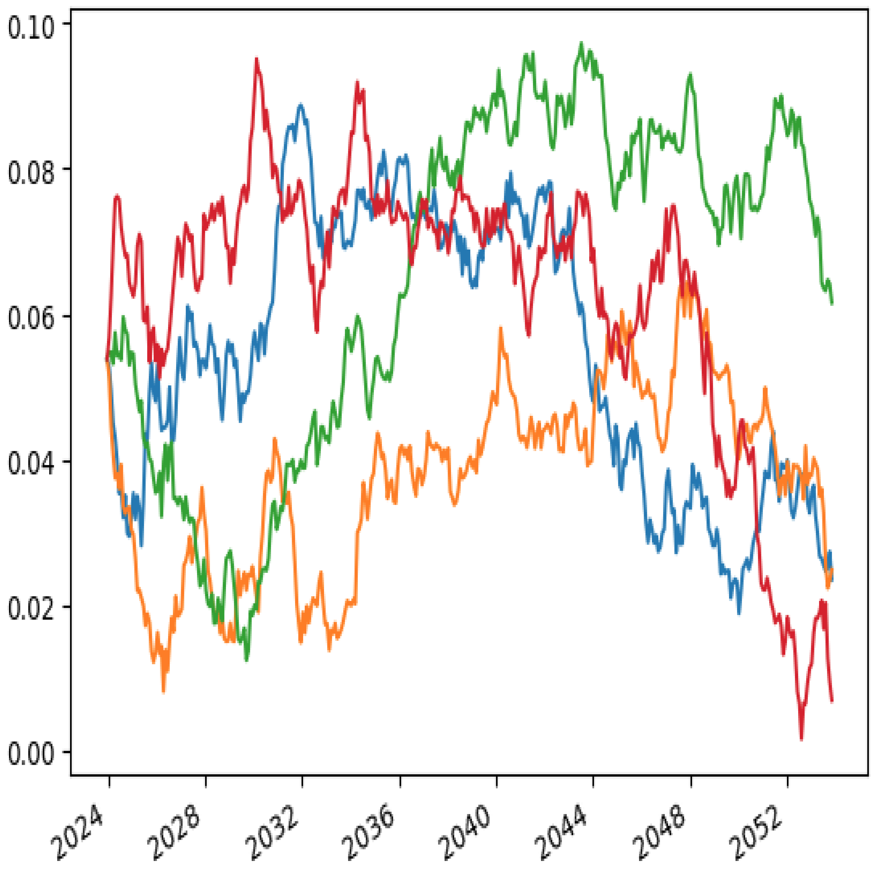
where κ denotes the mean reversion speed, θ ( t ) denotes the long-run mean of the interest rate, and σ r ( t ) controls the randomness of the short rate. The model is calibrated using the yield curve and interest rate volatility (see Andersen and Piterbarg 2010 for details) with market data from January 2024. Specifically, κ , θ ( t ) , and σ r ( t ) are chosen to fit the initial yield curve and the market available bond options and swaptions, using the analytical valuation formula for these instruments. While deposits typically have short maturities—leading to short-term simulations for both the short rate and deposit rate—mortgage loan maturities are significantly longer. To address the potential mismatch between deposit and loan maturities, we extend the simulation over a longer time horizon. Figure 3 presents several simulated short-rate scenarios over a 30-year period (from January 2024 to January 2054) under this model. The short rate exhibits mean reversion and time-varying volatility.
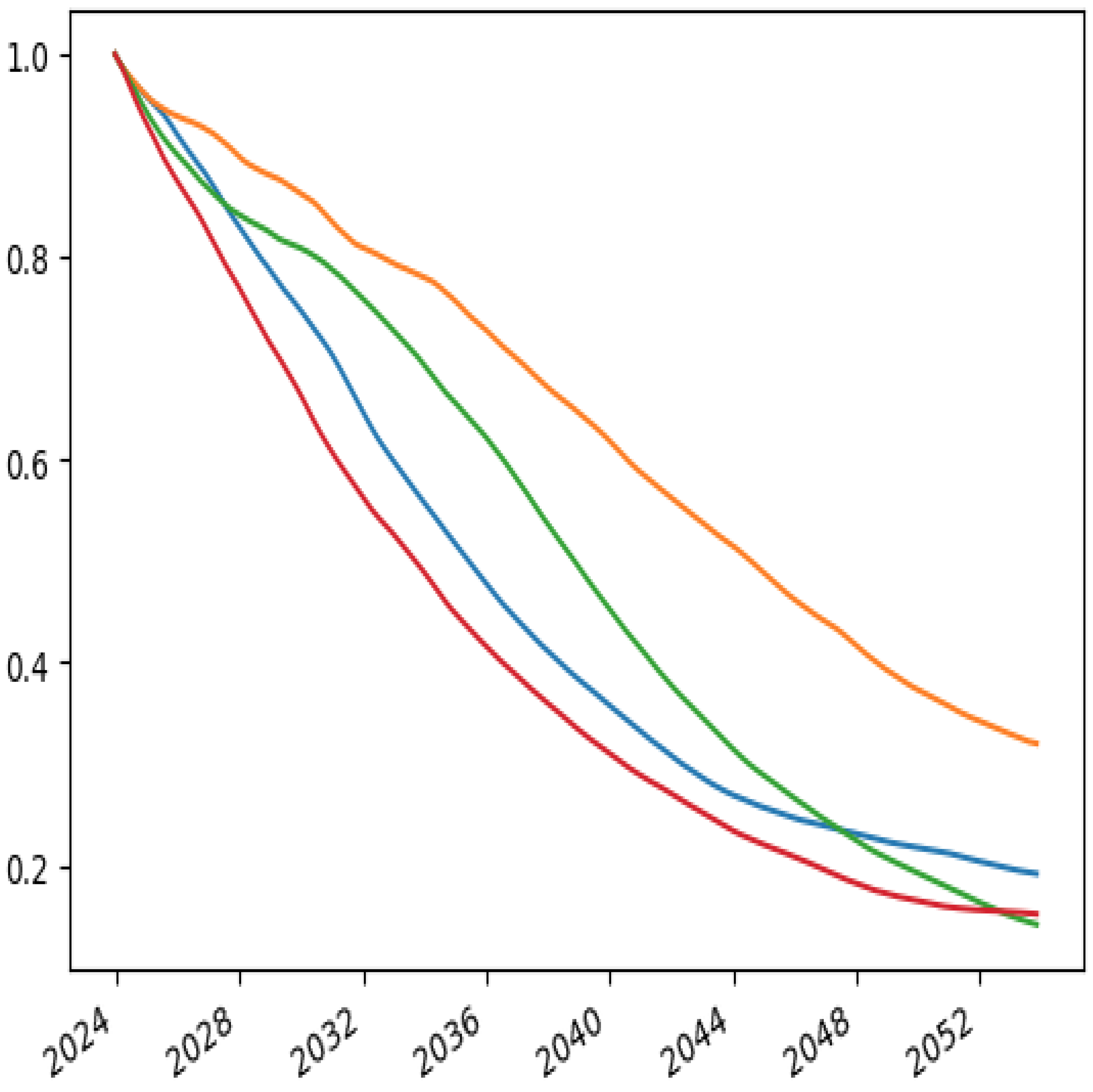
We begin by examining the liability side of the balance sheet, focusing on deposit balances. Figure 4 presents multiple simulations of deposit balances, each corresponding to a different possible trajectory of the short-term interest rate. We categorize deposits by size and assume a decay rate of 50%, meaning that deposits gradually leave the bank over time within a given deposit account. This outflow may result from customer withdrawals, account closures, or the reallocation of funds to higher-yield alternatives. For simplicity, we assume no new deposits (i.e., no inflows) for a single deposit account. The initial balance is set at 1 million, representing the starting deposit pool.
As shown in Figure 4, even though the decay rate itself is fixed, the deposit balance still varies across different simulations because interest rate dynamics influence customer behavior and cash flow timing. Higher short-term interest rates might accelerate withdrawals, while lower rates might slow them down, even in the absence of explicit behavioral modeling. Since there is no new money flowing in, deposits naturally decline over time due to the assumed outflows. This reflects a key liquidity risk consideration—if deposits are steadily decreasing, the bank must manage its funding sources carefully. Since each depositor cohort may behave differently depending on their individual deposit terms, interest rate sensitivity, and withdrawal patterns, it is important to simulate all deposit balances together (aggregate deposit) to understand how different groups of depositors affect overall funding stability. More generally, the parameter μ in Equation (15) can be calibrated to account for new balance growth.
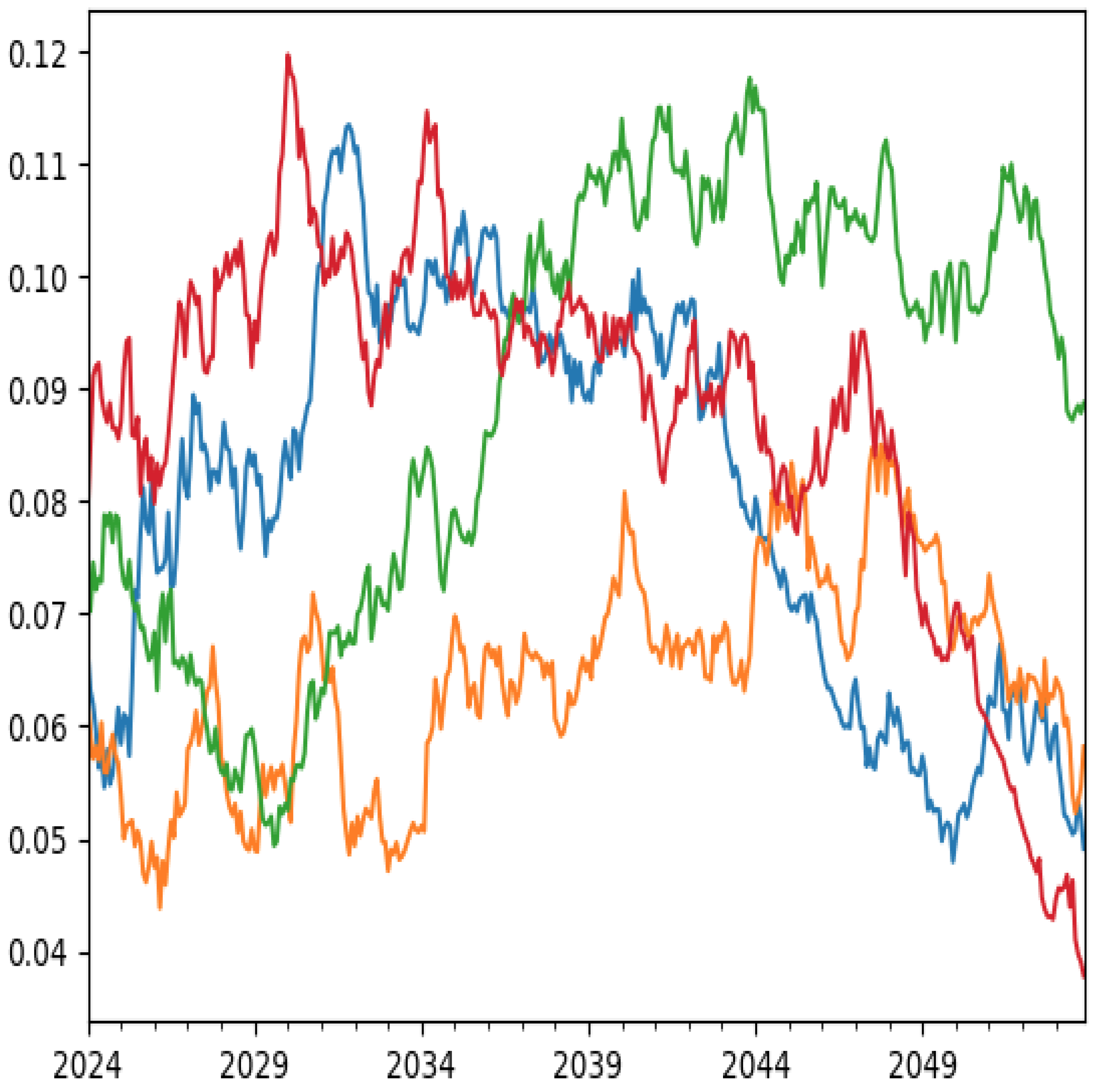
Next, we examine the long-maturity asset side of the balance sheet. We apply the same interest rate model to the asset side, specifically for mortgage loans. Figure 5 presents simulations of primary mortgage rates for 30 different mortgage cohorts within a prepayment model. Since the primary mortgage rate refers to the rate that borrowers pay on new mortgages, which evolves based on interest rate fluctuations, the primary mortgage rate is highly influenced by the interest rate scenario. Figure 5 illustrates simulations of mortgage rates for 30 different mortgage cohorts, reflecting different origination times and prepayment behaviors. The prepayment model in the simulation helps capture borrower behavior dynamics, which are critical for valuing mortgage-backed assets.
Finally, we simulate the mortgage balance using the same interest rate model and corresponding mortgage rates. Figure 6 presents simulated mortgage balances under different scenarios for a 7% coupon Fannie Mae Conventional Loan (FNCL) mortgage pool with 355 months remaining as of January 2024. For simplicity, we assume an initial mortgage balance of 1 million. If rates decline, borrowers refinance or prepay early, accelerating the reduction in mortgage balances. If interest rates decline, borrowers are more likely to refinance or prepay early, accelerating the reduction in mortgage balances. Conversely, if rates increase, fewer prepayments occur, and the mortgage pool remains outstanding for a longer period compared to a low-rate scenario. This prepayment behavior is clearly illustrated across different interest rate simulation scenarios in Figure 6. Collectively, Figure 3, Figure 5 and Figure 6 demonstrate the significant impact of interest rates on mortgage balances. For instance, a 1% decrease in the interest rate results in an approximate 25–30% decline in mortgage balances. In contrast, if the primary mortgage rate remains unchanged, the mortgage balance decreases by only about 8%.

6. Economic Value of Equity

In this section, we present the EVB, the value of an asset minus the liability, of a commercial bank based on the above valuations in the last two sections in one consistent model. We also study the duration and convexity of the asset and liability, respectively, and then the risk to the equity.
We let A t be the time t value of all assets (mortgage loans, long-term and short-term assets, and other assets). Let L t be the time t value of deposits, debts, and other liquidities (except the equity). The no-arbitrage price models of other assets and liquidities are constructed with interest rate and other fundamental factors, { r ( t ) , η ( t ) } . Then, the EVE is given by
E ( t ) = A t L t .
Similar to the duration of the deposit in Section 3, we can generalize the duration concept for the deposit for the mortgage loan and the equity as follows.
Specifically, the duration of the asset is given by
D ( A ) = E Q 0 T e x p 0 t r ( s ) + h ( s ) ) d s t N t ( c + p t I t ) d t V 0 .
Alternatively, we can discuss the effect of interest rates on assets and liabilities directly. For instance, consider a parallel shift on the initial yield curve by Δ basis points. Then, we can calculate the price change for the asset and liability as D 0 ( Δ ) D 0 Δ or V 0 ( Δ ) V 0 Δ , respectively. As explained in Section 2, a good asset management for the parallel shift risk of the interest rate is designed to minimize the difference between these two “effective durations” of the liability portfolio and asset portfolio. Similarly, we can consider the effect of one particular maturity rate or other economic factors in the model.
In this framework, we can construct and analyze the cash flow of asset, liability, and equity value using the same scenario of r ( t ) and η ( t ) . Therefore, the Value at Risk (VaR)-based capitals can be calculated in the system. More importantly, stress testing and CCAR can be easily implemented.

7. Conclusions

This paper introduces an integrated and comprehensive framework encompassing all financial products listed on the balance sheet of a commercial bank. On the liability side, deposit rates and deposit balances are determined using an equilibrium-based behavioral approach. Similarly, the asset side, including mortgage loans and associated securities, is modeled through a comparable no-arbitrage and behavioral framework. A key component of this system is a unified model of both deposits and loans, incorporating interest rates and economic factors. As a practical implication, banks can adjust deposit rates by x% to stabilize EVE in response to interest rate shock.
While mortgage loans have been extensively studied in the literature in such works as Fermanian (2013) and Chernov et al. (2018), this paper contributes to considering the valuation of mortgage loans and the valuation of deposits (as developed in Hutchison and Pennacchi 1996 and Jarrow and Deventer 1998) within a consistent framework. Unlike the traditional duration–convexity approach, our method effectively manages interest rate risks in the valuation of non-standard assets by leveraging modern asset pricing theory. Our simulation results illustrate the dynamics of both deposit and mortgage balances under the same interest rate model. The implementation of this comprehensive risk management system is both practical and efficient, integrating advanced financial engineering techniques with sophisticated risk management methodologies and tools.
From an asset pricing perspective, behavioral analysis and certain economic factors contribute to market incompleteness, as these risks cannot be fully hedged in financial markets. Therefore, estimating the risk premiums associated with these factors is crucial. Furthermore, an empirical study applying this methodology to a commercial bank—while comparing it to previous research that focuses only on assets or liabilities—would provide valuable insights into how these risks interact. However, we leave this for future research, as it requires a more detailed analysis and empirical validation.

Author Contributions

Each author contributes equally on the methodology, implementation, and writing of this paper. All authors have read and agreed to the published version of the manuscript.

Funding

This research received no external funding.

Data Availability Statement

This paper relies solely on public data. Yahoo finance, https://finance.yahoo.com. Bloomberg, https://www.bloomberg.com.

Conflicts of Interest

Author Gregory R. Hackworth and Michael R. Vandenberg were employed by the company Bulls-Eye Solutions, LLC. The remaining authors declare that the research was conducted in the absence of any commercial or financial relationships that could be construed as a potential conflict of interest.

Appendix A. Deposit Rate and Deposit Balance

In each period from time t to t + 1 , we denote D ( t ) as the total balance and D i ( t ) = ω i ( t ) D ( t ) as the balance in segment i. The interest rate in this period is r ( t ) . The deposit rate for segment i is r i d ( t ) , and the cost incurred for the service is c i . In our setting, w i ( t ) is predetermined up to time t for the following reasons. First, the bank cannot fully and directly determine the balance in each segment but can do so indirectly and partly with the deposit rate. Second, the proportional ω i ( t ) depends on exogenous behavior factors. Nevertheless, the total balance D ( t ) will be determined. We also need to determine the deposit rate as well in equilibrium. We also omit the script “t” if necessary.
First, the bank solves the following optimization problem:
max r i d , i = 1 , , N i = 1 N ω i ( r ( t ) r i d ( t ) c i ( t ) ) D .
By the first-order condition to the deposit rates, we obtain, for each segment,
ω i D + i = 1 N ω i ( r r i d c i ) D r i d = 0 .
Therefore, for each pair ( i , j ) of the segment,
ω i : ω j = D r i d : D r j d .
This fundamental equation (A3) states that the marginal effect of the deposit rate on the total aggregate balance is proportional to the segment balance in equilibrium.
We next consider a specification of the balance,
D t = e μ t k r ( t ) + i = 1 N k i r i d ( t ) + η ( t )
where μ denotes the growth rate of new balance, the parameters k , k i represent the load coefficient (or contribution) of each rate to the balance, and η ( t ) denotes other explanatory variables that contain no deposit rates in their expressions.
Given this specification, we obtain
D r i d : D r j d = k i : k j .
Equations (A3) and (A5) together imply that ω i : ω j = k i : k j , i j . Then, there exists a non-zero number l such that k i = l ω i , i = 1 , , N . The economic meaning of this parameter l is explained later.
We now consider the optimization problem in each segment to maximize the following objective:
max r i d ( r r i d c i ) ω i D ,
where the first-order equation implies
r r i d c i = D D r i d .
By using the above specification of the aggregate balance, we have
D D r i d = k r ( t ) + i = 1 N k i r i d ( t ) + η ( t ) k i .
Then, Equations (A7) and (A8) together imply
ω i ( r ( t ) r i d ( t ) c i ) = k l r ( t ) + i = 1 N ω i r i d ( t ) + η ( t ) l , i = 1 , , N .
We rewrite the linear equations in (A9) as follows:
2 ω 1 r 1 d ( t ) + ω 2 r 2 d ( t ) + + ω N r N d ( t ) = ω 1 ( r ( t ) c 1 ) k l r ( t ) η ( t ) l ω 1 r 1 d ( t ) + ω 2 r 2 d ( t ) + + 2 ω N r N d ( t ) = ω N ( r ( t ) c N ) k l r ( t ) η ( t ) l
Define
A = 2 ω 1 ω 2 ω N ω 1 2 ω 2 ω N ω 1 ω 2 2 ω N , B = ω 1 ( r ( t ) c 1 ) ω 2 ( r ( t ) c 2 ) ω N ( r ( t ) c N ) , e = 1 1 1 .
Then, the deposit rate vector is given by
r d ( t ) = A 1 B ( k γ r ( t ) + η γ ) A 1 e .
By the Sherman–Morrison formula (Rao 1965) and noticing that the total weight i = 1 N ω i = 1 , we obtain
A 1 = d i a g ( 1 ω 1 , , 1 ω N ) 1 N + 1 V e ,
where
V = 1 ω 1 1 ω N .
By straightforward calculation, we derive
r d ( t ) = k r ( t ) + η ( t ) ( N + 1 ) l V r i = 1 N ω i c i N + 1 V + U ,
where U = ( r c 1 , , r c N ) .
Equivalently, the equilibrium deposit rate is given by
r i d ( t ) = 1 1 ( N + 1 ) ω i k + l l r ( t ) η ( t ) ( N + 1 ) l ω i c i + ω i c i ( N + 1 ) ω i .
By plugging the equilibrium deposit rate of Equation (A12) into the expression of the aggregate balance and straightforward algebra, we obtain
D ( t ) = e μ t k + l N + 1 r ( t ) + η ( t ) l i ω i c i ( t ) N + 1 .
As for the cost structure, we let c i ( t ) = ζ i + ( 1 ρ i ) r ( t ) , where 1 ρ i is the deposit required reserve ratio and ζ i denotes the fixed cost. Define two constants as follows:
a 1 N + 1 k + l l , b a i ω i ( 1 ρ i ) N + 1 .
Therefore, the aggregate deposit balance is given by
D ( t ) = e μ t l b r ( t ) + η ( t ) N + 1 l N + 1 ω i ζ i .
Finally,
r i d ( t ) = 1 a ω i ( 1 ρ i ) + i = 1 N ω i ( 1 ρ i ) ( N + 1 ) ω i r ( t ) η ( t ) ( N + 1 ) l ω i ζ i + i = 1 N ζ i ω i ( N + 1 ) ω i .
To illustrate our theory and the economic meaning of the parameters { k , l } , we start with the following case:
(I) We first consider a situation in which the short rate has no contribution to η ( t ) .
Let
β i = 1 a ω i ( 1 ρ i ) + i ω i ( 1 ρ i ) ( N + 1 ) ω i
This number β i denotes the beta of the deposit rate to the short rate. Rewrite this equation as
b ω i = 1 β i ( 1 ρ i ) = ρ i β i 0 .
Using the total weight i = 1 N ω i = 1 , we obtain
b i 1 ρ i β i = 1 .
(II) We consider the situation that η ( t ) contains the information of the term structure. We write
η ( t ) = s 1 ( r ( t ) r ( t 1 ) ) + s 2 ( r ( t ) r ( t 1 ) ) 2 + η ¯ ( t )
where the first component captures the slope of the interest rate, the second component reflects the curvature of the interest rate curve, and the last component represents other explanatory variables. In this case, we obtain
r i d ( t ) = β i r ( t ) + β ^ i ( r ( t ) r ( t 1 ) ) η ¯ ( t ) γ ( N + 1 ) ω i ζ i + i ω i ζ i ( N + 1 ) ω i ,
where the beta coefficient with respect to the short rate in the period [ t , t + 1 ] is
β i = ρ i b ω i s 2 γ ( N + 1 ) ω i r ( t ) + r ( t 1 ) ,
and
β ^ i = s 2 r ( t 1 ) s 1 γ ( N + 1 ) ω i .
Since the parameters s 1 and s 2 capture the effect of the slope and the curvature of the interest rate curve on the aggregate demand, the entire term structure affects the beta of each deposit rate in this setting. For instance, when s 2 = 0 , there is no curvature effect of the short rate to the aggregate balance; then,
r i d ( t ) = ρ i b ω i r ( t ) s 1 γ ( N + 1 ) ω i ( r ( t ) r ( t 1 ) ) ζ i + i ω i ζ i ( N + 1 ) ω i .
Finally, we discuss the implication of positive effect on the aggregate balance and aggregate beta. The first condition on the aggregate balance implies
b > 1 N + 1 i = 1 N ζ i ω i ( t ) r ( t ) .
The second condition on the aggregate beta implies
b < 1 N 1 1 N + 1 ζ i ω i ( t ) r ( t ) .
If each ω i ( t ) is independent of the short rate, the above Equations (A17) and (A18) yield 0 < b < 1 N + 1 . In general, we obtain
i ζ i ω i ( t ) r ( t ) < 1 .
This means that the weighted cost beta is smaller than 1.

Appendix B. Interest Rate and Economic Factor Model

We follow Duffie et al. (2000) to build a Gaussian–jump Markov process X in some state space D R n , satisfying a well-defined stochastic differential equation
d X t = μ ( X t ) d t + σ ( X t ) d W t + d Z t ,
where W is an n-dimensional standard Brownian motion, μ : D R n , σ : D R n × n , and Z is a pure jump process whose jumps have a fixed probability distribution ν on R n and arrive with intensity { λ ( X t ) : t 0 } , for some λ : D [ 0 , ) .
We impose the following assumptions: as follows,
  • μ ( x ) = K 0 + K 1 x , for K = ( K 0 , K 1 ) R n × R n × n ;
  • ( σ ( x ) σ ( x ) ) i h = ( H 0 ) i j , for H 0 R n × n ;
  • λ ( x ) = l 0 + l 1 x ˙ , for l = ( l 0 , l 1 ) R × R n × n .
We allow the factors η ( t ) as a linear combination of X t . We assume that the short rate r ( t ) = ρ 0 + ρ 1 · x , for ρ = ( ρ 0 , ρ 1 ) R × R n × n . We also assume that the stochastic hazard rate of the decay, prepayment, or default probability distribution, introduced in this paper, have a linear specification of X t .
It is known that
ψ ( u , X t , t , T ) = E t e x p t T r ( X s ) d s e u · X T = e α ( t ) + β ( t ) · x
for certain time-dependent functions α ( t ) and β ( t ) . Moreover,
ϕ ( v , u , X t , t , T ) = E t e x p t T r ( X s ) d s ( v · X T ) e u · X T = e ( α ( t ) + A ( t ) + ( β ( t ) + B ( t ) ) · x
for two other time-dependent functions A ( t ) and B ( t ) . These functions can be used to calculate the mortgage loans in Section 3. In our deposit model (Section 3), we need to calculate
E t e x p t T r ( X s ) d s Q ( X T )
for a quadratic function Q ( · ) when the market shares are constant. In general, we need to calculate this kind of expectation for a general function X T .
Given the Gaussian feature of the model, we consider an equivalent forward T-measure in which the zero coupon bond maturing at T is a numeraire. Then,
E t e x p t T r ( X s ) d s Q ( X T ) = P ( t , T ) E t T Q ( X T ) .
The first component, P ( t , T ) , on the right hand of the last equation can be calculated via Equation (A21). The second component, X T , satisfies the same kind of SDE under the forward T-measure. Since the density function of X T under the forward T-measure is known, we can calculate the second component analytically or via Monte Carlo simulation. The above discussion can be also extended to a quadratic term structure model, say, r t is a quadratic function of X (see Boyle and Tian 1999 and Ahn et al. 2002).
We present one example to illustrate our analytical approach. Consider a Hull–White model of the short rate r t (an example of one-dimensional Gaussian model) such as
d r ( t ) = ( θ ( t ) α r ( t ) ) d r + σ d W t .
The zero curve can be fully calibrated by the function θ ( t ) , due to the affine expression in Equation (A21), as follows:
θ ( t ) = f ( 0 , t ) t + α f ( 0 , t ) + σ 2 2 α ( 1 e 2 α t )
Precisely, we have the following expression of the bond price:
P ( t , T ) = A ( t , T ) e x p B ( t , T ) r t
where B ( t , T ) = 1 e x p ( a ( T t ) ) a , and
A ( t , T ) = e x p t T θ ( u ) B ( u , T ) d u σ 2 2 a ( B ( t , T ) T + t ) σ 2 4 a B ( t , T ) 2 .
Let us calculate the following integral (as in the deposit model or the mortgage loan model):
E e x p 0 T r ( t ) d t Q ( r T ) = P ( 0 , T ) E T Q ( r T ) .
Under the risk-neutral measure, r T is normally distributed:
r T N r 0 e a T + 0 T θ ( t ) d t , 1 e x p ( 2 a T ) 2 a .
It is known that r T is also normally distributed under the forward T-measure. Specifically,
r T N r 0 e a T + 0 T θ ( t ) d t σ B ( t , T ) , 1 e x p ( 2 a T ) 2 a .
Then, we can calculate E T Q ( r T ) analytically for polynomial function Q ( · ) and via efficient approximation formula for other non-linear functions. This method applies to the quadratic term structure model as well as general affine-jump factor models.
Finally, for the nonlinear specification of p t in the prepayment model, there is no analytical expression though. Still, we can implement efficient simulation methods for the prepayment model within the system.

Notes

1
Regulators have long been closely monitoring these issues, with significant guidance provided by the Basel Committee on Banking Supervision (BCBS). See, for example, the discussion on interest rate risk in BCBS (2016). For a comprehensive review of regulatory risk management in commercial banks, refer to Tian (2017). Additionally, Basel III has introduced more stringent minimum capital requirements and regulatory capital buffers, as explained in Labonte and Scott (2023).
2
Here, A ( R ) denotes the asset value when the interest rate is R.
3
We discuss the difference between congenial and combative deposit rate in equilibrium in Hackworth et al. (2024). Here, we make use of the congenial assumptions for segments.
4
For instance, for one deposit account only, let r d ( t ) = f ( r ( t ) ) r ( t ) for a function f ( · ) , as in Greenwald et al. (2023), by viewing deposit rates behavior more like options; we can construct a specification of D ( t ) = D ( x , y ) for x = r ( t ) , y = r d ( t ) such that
( x y ) D y ( x , y ) | y = f ( x ) = D ( x , f ( x ) ) .
5
For instance, p t = x t + y t max ( 0 , m a b r t ) , as in Chernov et al. (2018).

References

  1. Ahn, Dong-Hyun, Robert F. Dittmar, and A. Ronald Gallant. 2002. Quadratic term structure models: Theory and evidence. Review of Financial Studies 15: 243–88. [Google Scholar] [CrossRef]
  2. Andersen, Leif B. G., and Vladimir V. Piterbarg. 2010. Interest Rate Modeling, (II): Term Structure Models. London: Atlantic Financial Products. [Google Scholar]
  3. Barr, Michael. 2023. Review of the Federal Reserve’s Supervision and Regulation of Silicon Valley Bank. Board of Governors of the Federal Reserve System. Available online: https://elischolar.library.yale.edu/cgi/viewcontent.cgi?article=4955&context=ypfs-documents2 (accessed on 1 December 2024).
  4. BCBS. 2016. Standards: Interest rate risk in the banking book. In Basel Committee on Banking Supervision Consultative Document. Basel: BCBS. [Google Scholar]
  5. Boyle, Phelim P., and Weidong Tian. 1999. Quadratic Interest Rate Models as Approximation to Effective Rate Models. Journal of Fixed Income 9: 69–80. [Google Scholar] [CrossRef]
  6. Chernov, Mikhail, Brett R. Dunn, and Francis A. Longstaff. 2018. Macroeconomic-Driven Prepayment Risk and the Valuation of Mortgage-Backed Securities. Review of Financial Studies 31: 1132–83. [Google Scholar] [CrossRef]
  7. Detemple, Jerome, and Weidong Tian. 2002. The Valuation of American Option for a Class of Diffusion Process. Management Science 48: 917–37. [Google Scholar] [CrossRef]
  8. Diamond, Douglas W., and Philip H. Dybvig. 1983. Bank Runs, Deposit Insurance and Liquidity. Journal of Political Economy 91: 401–19. [Google Scholar] [CrossRef]
  9. Drechsler, Itamar, Alexi Savov, and Philipp Schnabl. 2021. Banking on Deposits: Maturity Transformation Without Interest Rate Risk. Journal of Finance 76: 1091–143. [Google Scholar] [CrossRef]
  10. Duffie, Darrell, Jun Pan, and Kenneth Singleton. 2000. Transform Analysis and Asset ricing for Affine Jump-Diffusions. Econometrica 68: 1343–76. [Google Scholar] [CrossRef]
  11. Fermanian, Jean-David. 2013. A Top-Down Approach for Asset-Backed Securities: A Consistent Way of Managing Prepayment, Default and Interest Rate Risks. Journal of Real Estate Finance and Economics 46: 480–515. [Google Scholar] [CrossRef]
  12. Fisher, Lawrence, and Roman L. Weil. 1971. Coping with the Risk of Interest-Rate Fluctuations: Returns to Bondholders from Naïve and Optimal Strategies. Journal of Business 44: 408–31. [Google Scholar] [CrossRef]
  13. Greenwald, Emily, Sam Schulhofer-Wohl, and Josh Younger. 2023. Deposit Convexity, Monetary Policy, and Financial Stability. Federal Reserve Bank of Dallas. Available online: https://ssrn.com/abstract=4602078 (accessed on 1 December 2024).
  14. Hackworth, Gregory R., Weidong Tian, and Michael R. Vandenberg. 2024. Deposit Betas and Market Shares Across Banks. Journal of Finance and Banking Review. forthcoming. [Google Scholar]
  15. Hutchison, David E. 1995. Retail Bank Deposit Pricing: An Intertemporal Asset Pricing Approach. Journal of Money, Credit and Banking 27: 217–31. [Google Scholar] [CrossRef]
  16. Hutchison, David E., and George G. Pennacchi. 1996. Measuring Rents and Interest Rate Risk in Imperfect Markets: The Case of Retail Bank Deposits. Journal of Financial and Quantitative Analysis 31: 399–417. [Google Scholar] [CrossRef]
  17. Janosi, Tibor, Robert Alan Jarrow, and Ferdinando Zullo. 1999. An Empirical Analysis of the Jarrowe-van Deventer Model for Valuing Non-Maturity Demand Deposits. Journal of Derivatives 7: 8–31. [Google Scholar] [CrossRef]
  18. Jarrow, Robert A., and Donald R. Van Deventer. 1998. The Arbitrage-free Valuation and Hedging of Demand Deposits and Credit Card Loans. Journal of Banking and Finance 22: 249–72. [Google Scholar] [CrossRef]
  19. Karpishpan, Yakov, Ozgur Turel, and Alexander Hasha. 2010. Introducing the Citi LMM Term Structure Model for Mortgages. Journal of Fixed Income 20: 44–58. [Google Scholar] [CrossRef]
  20. Labonte, Marc, and Andrew P. Scott. 2023. Bank Capital Requirements: Basel III Endgame. CRS Report. Available online: https://crsreports.congress.gov/product/pdf/R/R47855 (accessed on 1 December 2024).
  21. Moulin, Serge. 2020. Modeling of N Maturity Deposits for IRRBB: Statistical or Behavioral Approach? ALM-Vision. Available online: https://www.researchgate.net/publication/344515893_Modeling_of_No_Maturity_Deposits_for_IRRBB_Statistical_or_behavioral_approach (accessed on 1 December 2024).
  22. Rao, Calyampudi Radhakrishna. 1965. Linear Statistical Inference and Its Applications. New York: Wiley. [Google Scholar]
  23. Sheehan, Richard G. 2013. Valuing Core Deposits. Journal of Financial Service 43: 197–220. [Google Scholar] [CrossRef]
  24. Stanton, Richard. 1995. Rational Prepayment and the Valuation of Mortgage-Backed Securities. Review of Financial Studies 8: 677–708. [Google Scholar] [CrossRef]
  25. Tian, Weidong. 2017. Commercial Banking Risk Management: Regulation in the Wake of the Financial Crisis, 1st ed. London: Palgrave Macmillan. [Google Scholar]
  26. Wyle, Robert J. 2014. Asset and Liability Management: Applications for Management and Modeling of Non-Maturing Deposits. New York: Moody’s Analytics. [Google Scholar]
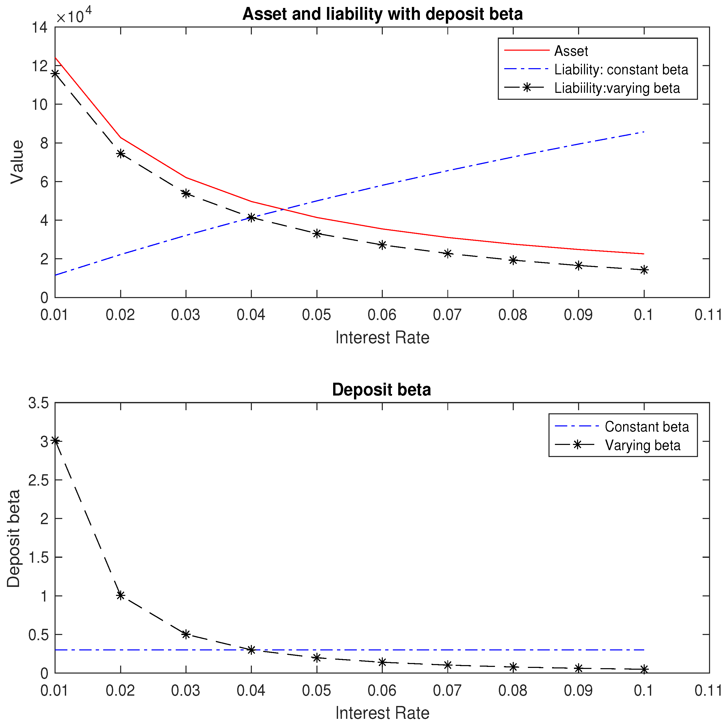
Figure 1. An example of asset and liability. In the top panel, we plot the values of assets and liabilities as the interest rate changes, comparing the liability value under two different deposit beta structures: constant and time-varying. In the bottom panel, we depict the deposit rate (in percentage) against the interest rate under both beta specifications.
Risks 13 00052 g001
Figure 2. An integrated risk management system. This figure provides an overview of the system’s structure, highlighting its key components and their interactions.
Risks 13 00052 g002
Figure 3. Simulations of 3-month short rate. This figure illustrates multiple scenarios of the 3-month short rate generated using a one-factor Gaussian interest rate model. The simulations begin in January 2024 and extend over a 30-year horizon. The model is calibrated based on the yield curve and interest rate volatilities.
Risks 13 00052 g003
Figure 4. Simulation of deposit balance. This figure illustrates the deposit balance of a deposit account under various interest rate scenarios. Depositors are categorized by deposit size, with an initial deposit balance of 1 million. The y-axis represents the balance in millions, while the x-axis denotes the time period from 2024 to 2054.
Risks 13 00052 g004
Figure 5. Simulation of primary mortgage rate. This figure illustrates multiple scenarios of primary mortgage rate from Jan 2024 to Jan 2054. The primary mortgage rate refers to the interest rate that lenders charge on home loans issued to borrowers, which are determined by the short-rate simulated in the one-factor Gaussian interest rate model.
Risks 13 00052 g005
Figure 6. Simulation of mortgage balance. This figure illustrates the mortgage balance of a 7% coupon FCNL mortgage with 355 months remaining as of January 2024. The initial mortgage loan balance is 1 million. The figure highlights the impact of interest rate fluctuations, particularly the primary mortgage rate, on the prepayment option and the resulting mortgage balance over time.
Risks 13 00052 g006
Disclaimer/Publisher’s Note: The statements, opinions and data contained in all publications are solely those of the individual author(s) and contributor(s) and not of MDPI and/or the editor(s). MDPI and/or the editor(s) disclaim responsibility for any injury to people or property resulting from any ideas, methods, instructions or products referred to in the content.