Distinguishing Log-Concavity from Heavy Tails

Abstract

Well-behaved densities are typically log-convex with heavy tails and log-concave with light ones. We discuss a benchmark for distinguishing between the two cases, based on the observation that large values of a sum $X_1+X_2$ occur as result of a single big jump with heavy tails whereas $X_1,X_2$ are of equal order of magnitude in the light-tailed case. The method is based on the ratio $|X_1-X_2|/(X_1+X_2)$, for which sharp asymptotic results are presented as well as a visual tool for distinguishing between the two cases. The study supplements modern non-parametric density estimation methods where log-concavity plays a main role, as well as heavy-tailed diagnostics such as the mean excess plot.

1. Introduction

General interest towards non-parametric thinking has increased over the last few years. One example is density estimation under shape constraints instead of requiring the membership of a parametric family. Here, a particularly robust alternative to parametric tests is provided by searching for the best fitting log-concave density. Another example is the mean excess plot that aims at distinguishing light and heavy tails.

Throughout the paper, we consider i.i.d. random variables $X,X_1,X_2,\dots >0$ with common distribution F having density f and tail $\overline{F}(x)=\mathbb{P}(X>x)$. Then, X is (right) heavy-tailed if $\mathbb{E}{\mathrm{e}}^{sX}=\infty$ for all $s>0$ and light-tailed otherwise. The density f is log-concave, if $f(x)={\mathrm{e}}^{\varphi (x)}$, where $\varphi$ is a concave function. If $\varphi$ is convex, then f is log-convex. This paper aims to illustrate that light-tailed asymptotic behaviour is associated with log-concave densities. Likewise, log-convexity seems to be connected to heavy-tailed behaviour. One can use the connection to assess potential heavy-tailedness by searching for patterns that are typically present among distributions with log-concave or log-convex densities.

Log-concavity is a widely studied topic in its own right [1,2]. There also exists substantial literature regarding its connections to probability theory and statistics [3,4]. Several papers concentrate on the statistical estimation of density functions assuming log-concavity [5,6]. This is due to the fact that log-concavity provides desirable statistical properties for estimators. For instance, maximum likelihood estimation becomes applicable and the estimate is unique. The topic is discussed in detail in the beginning of [7]. Unfortunately, much less emphasis seems to be put on verification of the log-concavity property itself. Specifically, it seems to be relatively little studied if it is feasible that the sample be generated by a log-concave distribution. See, for example [8,9].

A distribution with a log-concave density f is necessarily light-tailed. In contrast, f is log-convex in the tail in the standard examples of heavy tails such as regular variation, the lognormal distribution and Weibull case $\overline{F}(x)={\mathrm{e}}^{-x^{\alpha }}$ with $\alpha <1$. An important class of heavy-tailed distributions are the subexponential ones defined by $\mathbb{P}(X_1+X_2>d)\sim 2\overline{F}(d)$. The intuition underlying this definition is the principle of a single big jump: $X_1+X_2$ is large if one of $X_1,X_2$ is large, whereas the other remains typical. This then motivates

$$R=\frac{|X_1-X_2|}{X_1+X_2}$$

(1)

being close to 1. In contrast, the folklore is that $X_1,X_2$ contribute equally to $X_1+X_2$ with light tails. We are not aware of general rigorous formulations of this principle, but it is easily verified in explicit examples like a gamma or normal F (see further below) and, for a large number of summands rather than just 2, it is supported by conditioned limit theorems (see e.g., ([10] (VI.5))). However, it was recently shown in [4] that these properties of R hold in greater generality and that asymptotic properties of the corresponding conditioned random variable

$$Y_d=R|X_1+X_2>d$$

(2)

provide a sharp borderline between log-convexity and log-concavity.

In this paper, we provide a wider perspective in terms of both sharper and more general limit results and of the usefulness for visual statistical data exploration. To this end, we propose a feature based nonparametric test. It can be used as a visual aid in identification of log-concavity or heavy-tailed behaviour. It complements earlier ways to detect signs of heavy-tailedness such as the mean excess plot [11]. Further tests based on probabilistic features have been previously utilised in e.g., [12,13,14].

2. Background

A property holds eventually, if there exists a number $y_0$ so that the property holds in the set $[y_0,\infty )$. Standard asymptotic notation is used for limiting statements. These and basic properties of regularly varying functions with parameter α, denoted RV(α), can be recalled from e.g., [15].

We note that the principle of a single big jump relates to the fact that joint distributions of independent random variables concentrate probability mass to different regions. For example, a distribution with tail function $\overline{F}(x)={\mathrm{e}}^{-x^{\alpha }}$ satisfies

$$\overline{F}(x)=\mathrm{o}(\overline{F}{(x/2)}^2)$$

for $\alpha >1$ and

$$\overline{F}{(x/2)}^2=\mathrm{o}(\overline{F}(x))$$

for $\alpha \in (0,1)$, as $x\to \infty$. We refer to [16,17,18,19] for related work in this direction. It is shown in Lemma 1.2 of [4] that log-concavity or log-concavity of the density is closely related to the occurrence of the principle of a single big jump. A further observation in this direction is the following lemma. It states that contour lines of joint densities of independent variables behave differently for log-concave and log-convex densities, and thereby leads naturally to different concentrations of probability mass of joint densities (recall that a contour line corresponding to a value $p\in \mathbb{R}$ of joint density $f:{\mathbb{R}}^2\to \mathbb{R}$ is the set of points in the plane defined as $\{(x,y)\in {\mathbb{R}}^2:f(x,y)=p\}$).

Lemma 1.

Suppose $X_1$ and $X_2$ are i.i.d. unbounded non-negative random variables. Assume further that they have a common twice differentiable density function f of the form

$$f(x)={\mathrm{e}}^{-h(x)},$$

where h is a strictly increasing function.

If f is log-concave (log-convex), then, for any fixed $p\in (0,{\mathrm{e}}^{-h(0)})$, there exists a convex (concave) function ${\psi }_p$ defining a contour line of $f_{X_1,X_2}$ corresponding to p such that $f_{X_1,X_2}(x,{\psi }_p(x))=p$ for all $x\in [0,h^{-1}(-logp-h(0))]$.

Lemma 1 implies that log-convex and log-concave densities cause maximal points of joint densities to accumulate into different regions in the plane. Log-convex densities tend to put probability mass near the axis, while log-concave densities have a tendency to concentrate mass near the graph of the identity function. The exponential density is the limiting case where all contour lines are straight lines. More generally, for $f_{\alpha }(x)=C_{\alpha }{e}^{-x^{\alpha }}$, where $C_a>0$ is an integration constant, the contour lines are circles for $\alpha =2$, straight lines for $\alpha =1$, and parabolas for $\alpha =1/2$.

3. Theoretical Results

The emphasis of the paper is on the mathematical formulation of the connection between log-convexity and the principle of a single big jump. However, some additional theoretical results are provided concerning convergence rates of the conditional ratio defined in Equation (3). These rates, or estimates for the rates, are obtained in some standard distribution classes. Their proofs are mainly based on sharp asymptotics of subexponential distributions obtained in [20,21,22]. Recall that some main classes of such distributions are RV$(\alpha )$, meaning regularly varying ones, where $\overline{F}(x)=L(x)/x^{\alpha }$ with $\alpha >0$ and $L(·)$ are slowly varying, Weibull tails with $\overline{F}(x)={\mathrm{e}}^{-x^{\alpha }}$ for some $\alpha \in (0,1)$, and lognormal tails which are close to the case $\gamma =2$ of $\overline{F}(x)={\mathrm{e}}^{-{log}^{\gamma }x}$ for $x\ge 1$ and some $\gamma >1$; we refer in the following to this class as lognormal type tails.

3.1. Convergence Properties

Define the function $g:(0,\infty )\to [0,1]$ by

$$g_X(d)=g(d)=\mathbb{E}\left[\frac{|X_1-X_2|}{X_1+X_2}|X_1+X_2>d\right].$$

(3)

It can be viewed as a generalisation of the function $f_{Z_d}$ considered in [4] and has the same interpretation as in the case with densities: if both $X_1$ and $X_2$ contribute equally to the sum $X_1+X_2$, then g should eventually obtain values close to 0; similarly, if only one of the variables tends to be the same magnitude as the whole sum, then g is close to 1 for large d. Note also that g is scale independent in the sense that $g_{aX}(d)=g_X(d/a)$ for all $a>0$. Due to this property, two or more samples can be standardised to have, say, equal means in order to obtain graphs on the same scale.

In Proposition 1, sharp asymptotic forms of g are exhibited in some classes of distributions.

Proposition 1.

The following convergence rates hold for g defined in Equation (3).

• Let X be RV$(\alpha )$ with $\alpha >1$, eventually decreasing density f. Then,

  $$g(d)=1-\frac{c}{d}+\mathrm{o}(1/d)\mathit{where}c=\frac{2\alpha \mathbb{E}[X]}{\alpha +1}.$$
• Let X be Weibull distributed with $\alpha <1$. Then,

  $$g(d)=1-\mathrm{o}(d^{\alpha -1}).$$

  (4)
• Let X be of lognormal type. Then,

  $$g(d)=1-\mathrm{o}({log}^{\gamma -1}x/x).$$

  (5)

Remark 1.

In the case of Weibull and lognormal distributions, the implication is that $g(d)$ converges to 1 at a larger rate than their associated hazard rates tend to zero. In addition, inspection of the proof shows

$$\underset{d\to \infty }{lim\; inf}d\left|g(d)-1\right|>0.$$

This implies that the actual convergence rate can not be substantially larger than in the regularly varying case, where the leading term is explicitly identified.

The light-tailed case appears to be more difficult to study than the heavy-tailed case. Difficulty arises mainly from the lack of good asymptotical approximations for probabilities of the form $\mathbb{P}(X_1+X_2>d)$ when $\mathbb{P}(X_1>d)$ decays much faster than $e^{-d}$. Interestingly, the full asymptotic form of g can be recovered in the special case of the normal distribution if we allow X to obtain negative values.

Proposition 2.

Suppose that X is normally distributed with $\mathbb{E}[X]=0$ and $\mathbb{V}ar[X]=1/\sqrt{2}$. Then,

$$g(d)=\frac{c}{d}+\mathrm{o}(1/d),\mathit{where}c=\mathbb{E}\left[|X_1-X_2|\right].$$

(6)

The following theorem can be used to assess if a sample is coming from a source with log-concave density. It can be seen as a natural continuation as well as a generalisation to [4].

Theorem 1.

Assume the density f is twice differentiable and eventually log-concave. Then,

$$\underset{d\to \infty }{lim\; sup}g(d)\le \frac{1}{2}.$$

(7)

Similarly, if f is eventually log-convex, then

$$\underset{d\to \infty }{lim\; inf}g(d)\ge \frac{1}{2}.$$

(8)

4. Statistical Application: Visual Test

Suppose $(X_1,Y_2),(X_2,Y_2),\dots$ is a sequence of i.i.d. vectors whose components are also i.i.d. One can formulate the empirical counterpart of Quantity (3) by setting

$$\widehat{g}(d,n)=\frac{{\displaystyle \sum _{k=1}^n{R}_k\mathbf{1}(X_k+Y_k>d)}}{{\displaystyle \sum _{k=1}^n\mathbf{1}(X_k+Y_k>d)}},$$

(9)

where

$$R_k=\frac{|X_k-Y_k|}{X_k+Y_k},$$

and $\mathbf{1}(A)$ is the indicator function of the event A.

Remark 2.

Equation (9) requires as input a two-dimensional sequence of random variables. One can form such a sequence from a real valued i.i.d. source $Z_1,Z_2,\dots ,Z_N$ using any pairing of the $Z_i$. Obvious examples are to take $X_k=Z_{2k-1},Y_k=Z_{2k}$ to take the set $\left\{(X_k,Y_k)\right\}$ as all pairings of the $Z_k$ or as a randomly sampled subset of these $N(N-1)/2$ pairings. If the data is truly i.i.d, this should not have any effect on the outcome.

4.1. Examples and Applications

A graph of $\widehat{g}(d,n)$ as function of d can be used to determine if the data support the density being log-concave or light-tailed behaviour. According to Theorem 1, the graph should then stay below $1/2$. Figure 1, Figure 2, Figure 3 and Figure 4 illustrate such graphs using experimental data.

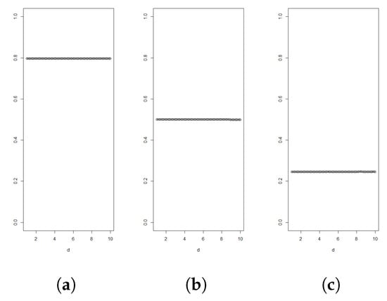
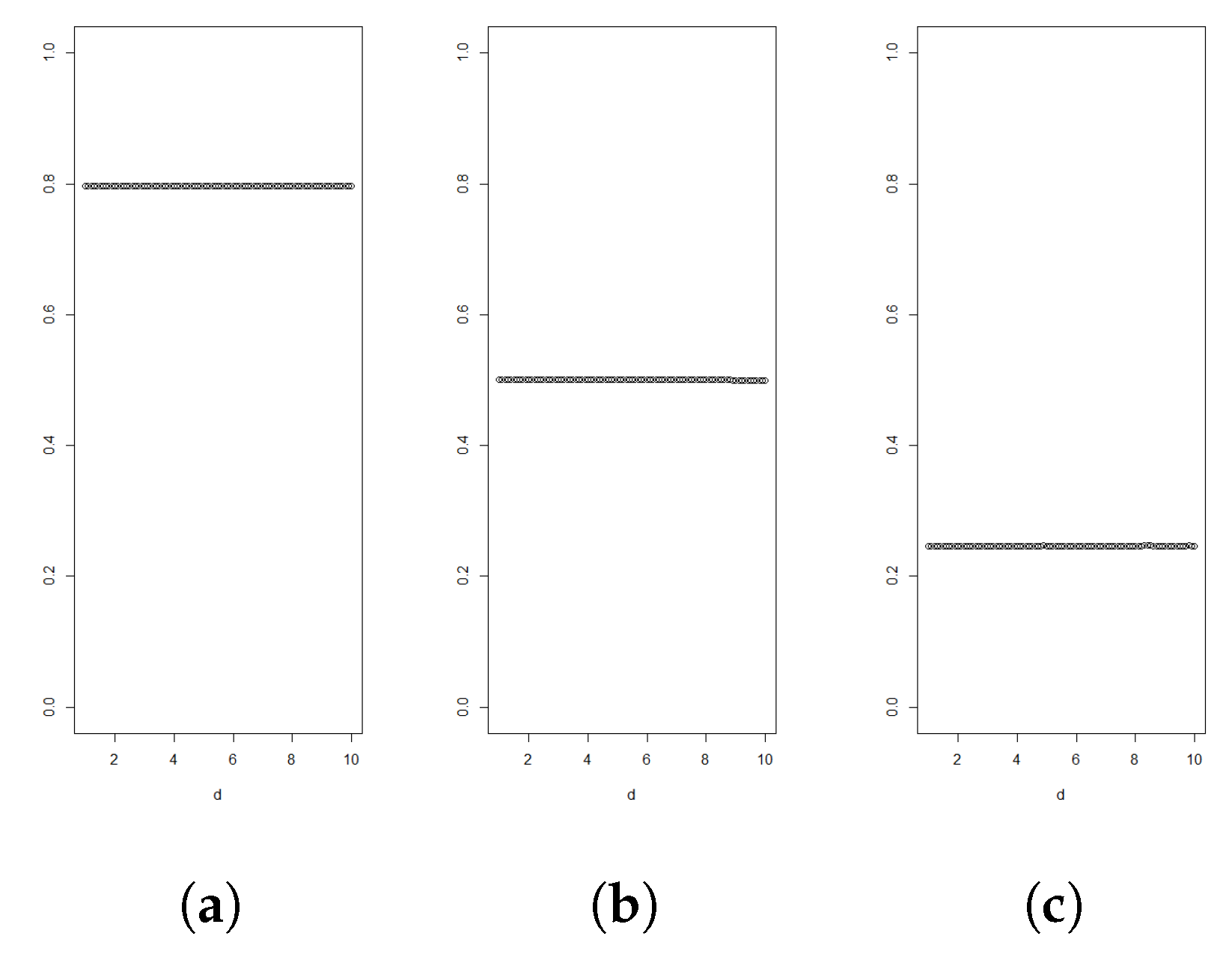
Figure 1. Graphs of $\widehat{g}(d,n)$ for $n=10,000$ for Gamma distributed random variables with shapes $0.2,1$ and 5 in figures (a), (b) and (c), respectively. All variables are standardised to have mean 3.

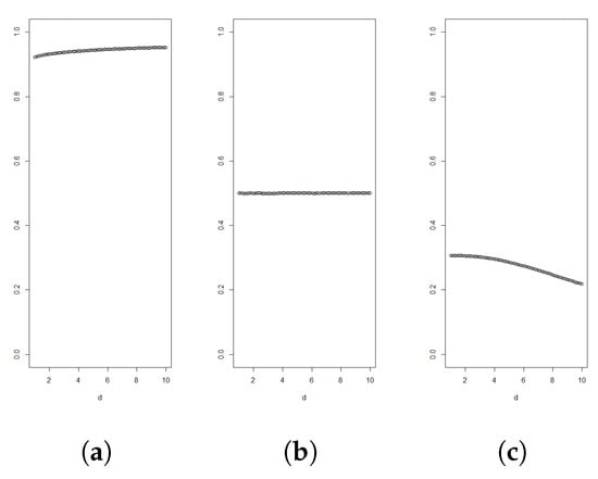
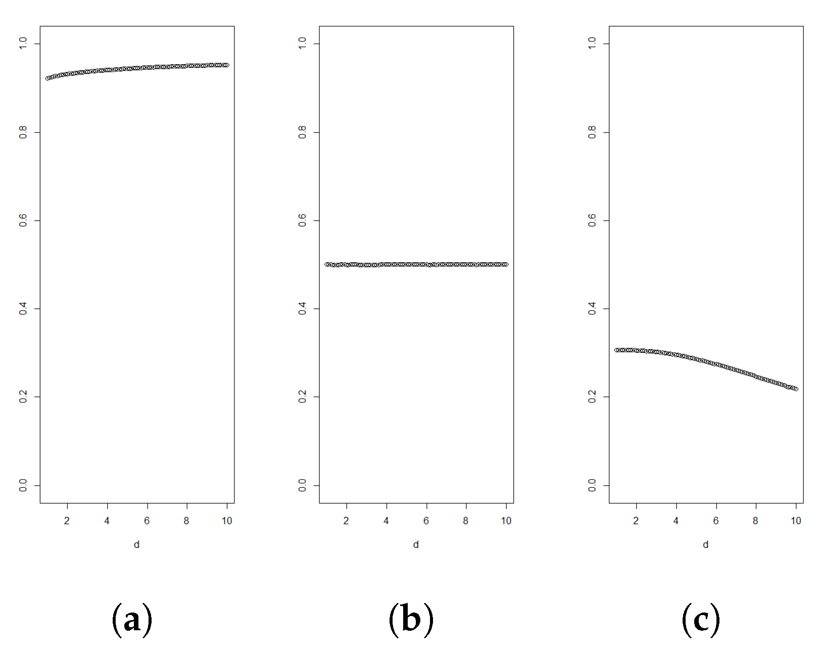
Figure 2. Graphs of $\widehat{g}(d,n)$ for $n=10,000$ for Weibull distributed random variables with shapes $0.2,1$ and 5 in figures (a), (b) and (c), respectively. All variables are standardised to have mean 3.

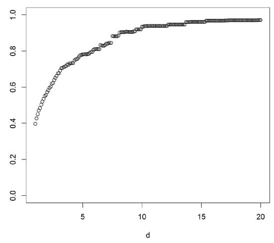
Figure 3. Graph of $\widehat{g}(d,n)$ from a classical set of Danish fire insurance data that can be obtained for instance from data set ‘danish’ in the R package [23]. The data is scaled to have mean 1. The sample is traditionally used to illustrate how heavy-tailed data behaves. A similar set of data was previously used in [24]. The graph supports the usual finding that the data set is heavy-tailed.

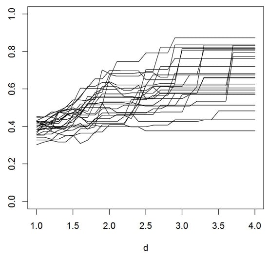
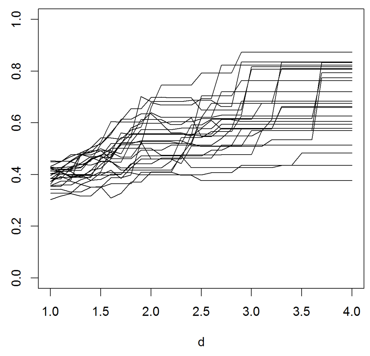
Figure 4. The graphs of multiple versions of $\widehat{g}(d,n)$ based on a dataset obtained from Hansjörg Albrecher (private communication) and related to occurrences of floods in a particular area. The data is scaled to have mean 1. The sample size is $n=39$. Bivariate vectors $(X_1,Y_1),\dots ,(X_{19},Y_{19})$ were sampled several times randomly without replacement from the original data. The overall appearance of the paths points to the data being heavy- rather than light-tailed.

The test method is visual. A similar idea has been used at least in the classical mean excess plot, where one visually assesses if the tail excess in the sample points is increasing at the level, as is the case for heavy tails.

4.2. Finer Diagnostics

The idea of plotting $\widehat{g}(d,n)$ as a function of d was introduced as a graphical test for distinguishing between heavy-tailed and log-concave light tailed distributions. It seems reasonable to ask if the plot can be used for finer diagnostics, in particular to further specify the tail behaviour of F when F was found to be heavy-tailed. Such an idea would be based on the rate of convergence of $\widehat{g}(d,n)$ to 1.

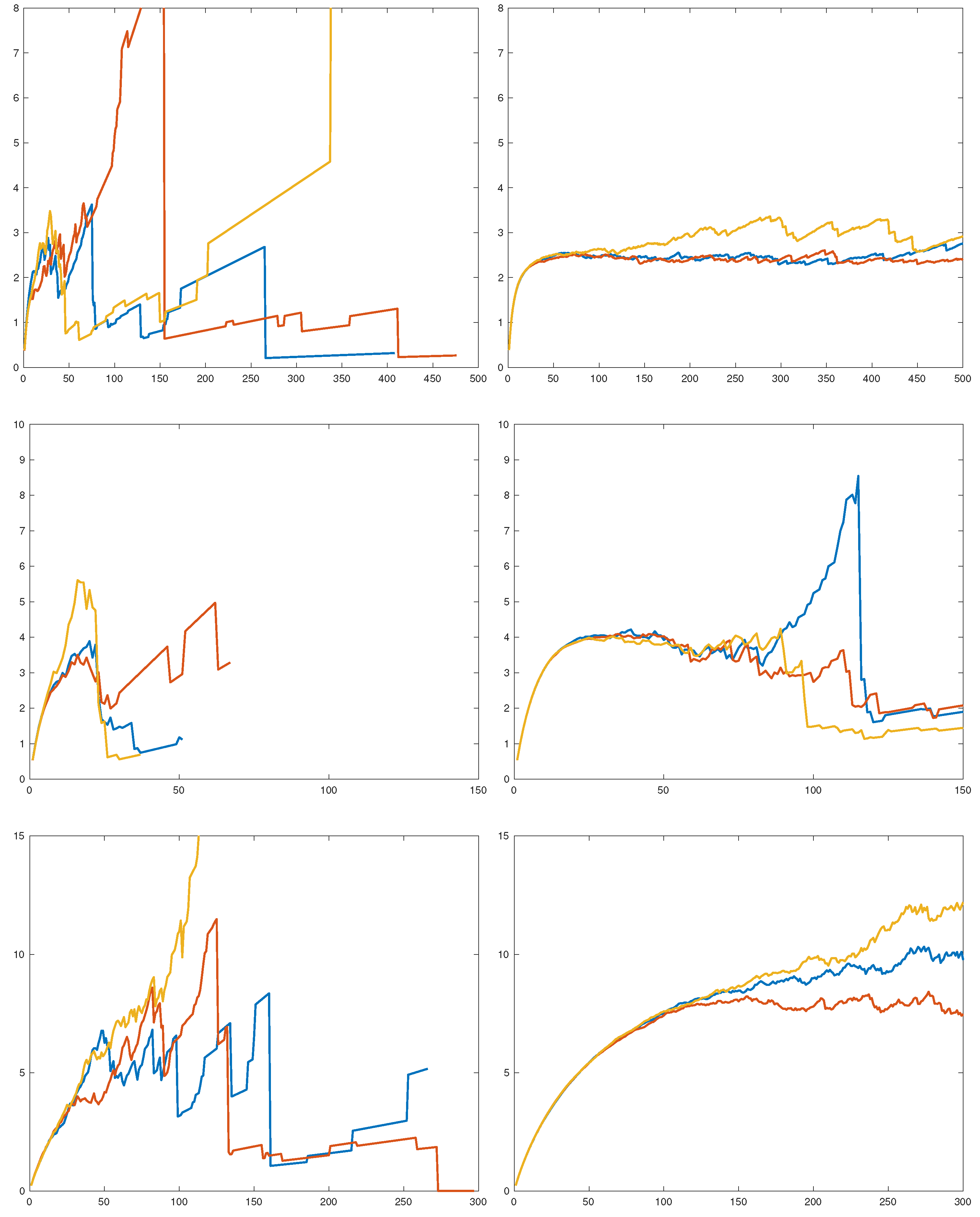
To gain some preliminary insight, we simulated $R=5000=5·{10}^3$ and $R=5·{10}^6$ i.i.d pairs of r.v.’s $X_1,X_2$ from an F which was either RV(1.5), lognormal(0,1) or Weibull(0.4). The results are in Figure 5 as plots of $d\left(1-\widehat{g}(d,n)\right)$, with three runs in each subfigure.

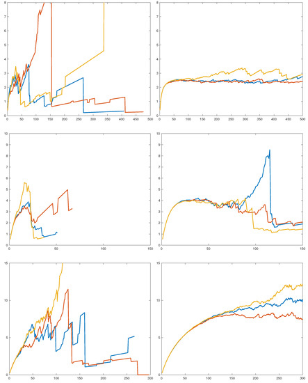
Figure 5. $d\left(1-\widehat{g}(d,n)\right)$. Pareto in the first row, lognormal in the second, and Weibull in the last. $R=5000$ (left), $R=5\times {10}^6$ (right).

A first conclusion is that a sample size of $R=5000$ is grossly insufficient for drawing conclusions about the way in which $\widehat{g}(d,n)$ approaches 1—random fluctuations take over long before a systematic trend is apparent. The sample size $R=5·{10}^6$ is presumably unrealistic in most cases, but even for this, the picture is only clear in the RV case. Here, $d\left(1-\widehat{g}(d,n)\right)$ seems to have a limit c, as it should be, and the plot is in good agreement with the value 2.4 = $2\alpha \mathbb{E}[X]/(\alpha +1)$ of c predicted by Proposition 1.

Whether a limit exists in the lognormal or Weibull case is less clear. The results of Proposition 1 are less definite here, but, actually, a heuristic argument suggests that the limit c should exist and be $2\mathbb{E}[X]$. To this end, let $X_{(1)}<X_{(2)}$ be the order statistics. According to subexponential theory (see, in particular, [25]), $X_{(1)},X_{(2)}$ are asymptotically independent given $X_1+X_2>d$, with $X_{(1)}$ having asymptotic distribution F and $X_{(2)}$ being of the form $d+e(d)E$ with $e(d)$, and E as in the proof of Proposition 1. For large d, this gives

$$\begin{array}{cc}\hfill \frac{|X_1-X_2|}{X_1+X_2}& \sim \frac{X_{(2)}-X_{(1)}}{X_{(2)}}\sim \frac{1-X_{(1)}/X_{(2)}}{1+X_{(1)}/X_{(2)}}\sim 1-2X_{(1)}/X_{(2)}.\hfill \end{array}$$

(10)

In the lognormal or Weibull case, one has $e(d)=\mathrm{o}(d)$ and so $d+e(d)E\sim d$. Taking expectations gives the conjecture.

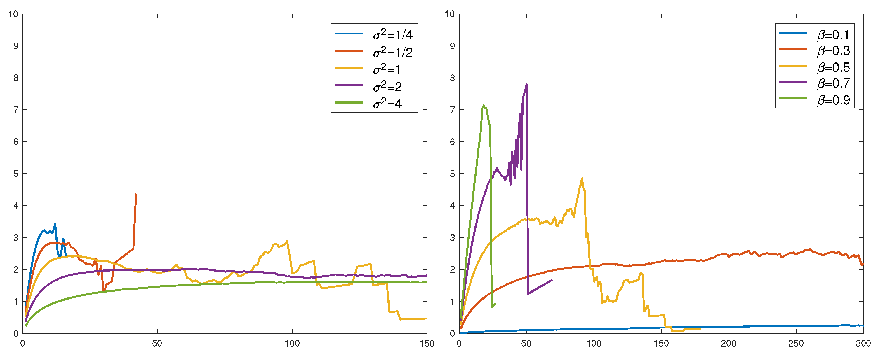
For the Weibull, $2\mathbb{E}[X]=6.65$, and the $R=5·{10}^6$ part of Figure 5 is rather inconclusive concerning the conjecture. We did one more run with $R=5·{10}^7$ over a range of parameters (the variance ${\sigma }^2$ of $logX$ for the lognormal and β for the Weibull). All $X_1,X_2$ were normalized to have mean 1 so that the conjecture would assert convergence to $c=2$. This is not seen in the results in Figure 6. Large values of ${\sigma }^2$ and small values of β could appear to give convergence, but not to 2.

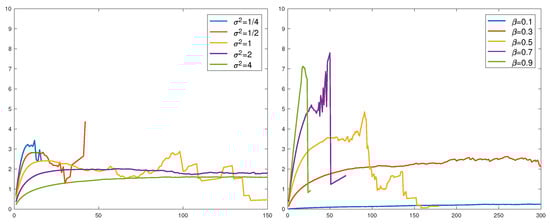
Figure 6. $R=5\times {10}^7$. Lognormal (left), Weibull (right).

It should be noted that the heuristics give the correct result in the RV case. Namely, here we can take $e(d)=d$ and $\mathbb{P}(E>x)=1/{(1+x)}^{\alpha }$. This easily gives $\mathbb{E}1/(1+E)=\alpha /(\alpha +1)$ so that Quantity (10) is approximately $1-2\alpha \mathbb{E}[X]/d(\alpha +1)$, as rigorously verified in Proposition 1.

The overall conclusion is that the finer diagnostic value of the method is quite limited, and restricted to RV and sample sizes which may be unrealistically large in many contexts.

5. Proofs

Proof of Lemma 1.

Suppose h is concave and $p\in (0,1)$. The contour line corresponding to value p is formed as the set of points $(x,y)$ that satisfy $f_{X_1,X_2}(x,y)=p$, or equivalently

$$h(x)+h(y)=-logp.$$

(11)

For any such pair $(x,y)$ one can solve Equation (11) for y to obtain

$$y=h^{-1}(-logp-h(x)).$$

(12)

Firstly, $h^{-1}$ is convex as the inverse of an increasing concave function. Secondly, the composition of an increasing convex function and a convex function remains convex. Thus, as a function of x, Expression (12) defines a convex function when $x\in [0,h^{-1}(-logp-h(0))]$. Thus, one can define ${\psi }_p(x)=h^{-1}(-logp-h(x))$.

If h is convex, the proof is analogous. ☐

The following technical lemma is needed in the proof of Proposition 1. It applies to Pareto, Weibull and lognormal type distributions. Indeed, condition (13) follows from Proposition 1.2; (ii) of [21] and further needed assumptions are easily verified apart from strong subexponentiality, which is known to hold in the mentioned examples.

Lemma 2.

Suppose $X_1$ and $X_2$ are non-negative i.i.d. variables with a common density f, where the hazard rate $r(d)=f(d)/\overline{F}(d)$ is eventually decreasing with $r(d)=\mathrm{o}(1)$. Assume further that

$$\mathbb{P}(X_1+X_2>d)-2\mathbb{P}(X_1>d)\sim 2\mathbb{E}[X]f(d).$$

(13)

Then,

$$\frac{2\mathbb{P}(X_1>d)+2f(d)\mathbb{E}[X]}{\mathbb{P}(X_1+X_2>d)}=1+\mathrm{o}(r(d)).$$

(14)

If in addition $\overline{F}{(d/2)}^2=\mathrm{o}(\overline{F}(d))$, then

$$\frac{\mathbb{P}(X_1\le d/2,X_2\le d,X_1+X_2>d)}{\mathbb{P}(X_1>d)}=\mathbb{E}[X]r(d)+\mathrm{o}(r(d)).$$

(15)

Proof. 

Equality (13) implies subexponentiality of $X_1$. Writing

$$\frac{2\mathbb{P}(X_1>d)+2\mathbb{E}[X]f(d)}{\mathbb{P}(X_1+X_2>d)}=1+\frac{-(\mathbb{P}(X_1+X_2>d)-2\mathbb{P}(X_1>d))+2\mathbb{E}[X]f(d)}{\mathbb{P}(X_1+X_2>d)}$$

and observing that the nominator on the right-hand side is of order $\mathbb{E}[X]r(d)\mathrm{o}(1)2\overline{F}(d)$ proves Equation (14) since $2\mathbb{P}(X_1>d)/\mathbb{P}(X_1+X_2>d)\to 1$ by subexponentiality.

Equality (13) implies

$$\begin{array}{ccc}\hfill \frac{\mathbb{P}(X_1+X_2>d)}{2\mathbb{P}(X_1>d)}& =& 1+\frac{2\mathbb{E}[X]f(d)(1+\mathrm{o}(1))}{2\mathbb{P}(X_1>d)}\hfill \\ & =& 1+\mathbb{E}[X]r(d)+\mathrm{o}(r(d)).\hfill \end{array}$$

(16)

On the other hand, writing

$$\begin{array}{ccc}\hfill \{X_1+X_2>d,X_2>X_1\}& =& \{X_1\le d/2,X_2>d\}\hfill \\ & \cup & \{X_1\le d/2,X_2\le d,X_1+X_2>d\}\hfill \\ & \cup & \{X_1>d/2,X_2>d/2\}\hfill \\ & =& A_1\cup A_2\cup A_3\hfill \end{array}$$

gives

$$\frac{\mathbb{P}(X_1+X_2>d)}{2\mathbb{P}(X_1>d)}=\frac{2\mathbb{P}(A_1)+2\mathbb{P}(A_2)+\mathbb{P}(A_3)}{2\mathbb{P}(X_1>d)}=1+\frac{\mathbb{P}(A_2)}{\mathbb{P}(X_1>d)}+\mathrm{o}(r(d)).$$

Since we know from Equation (16) that the leading term tending to zero must be $\mathbb{E}[X]r(d)$, Equation (15) holds. ☐

Proof of Proposition 1.

Suppose X is regularly varying with index α. In light of Lemma 2, we only need to establish

$$\mathbb{E}\left[\frac{X_1-X_2}{X_1+X_2};X_1>X_2,X_1+X_2>d\right]=\overline{F}(d)\left(1-\frac{c}{d}+\frac{\alpha }{d}\mathbb{E}X+\mathrm{o}(1/d)\right).$$

(17)

The contribution to the l.h.s of Equation (17) from

$$\mathbb{E}\left[\frac{X_1-X_2}{X_1+X_2};X_1>X_2,X_2>Ad,X_1+X_2>d\right]$$

is of order $O\left(\overline{F}(d/2)\overline{F}(Ad)\right)=O\left(d^{-2\alpha +ϵ}\right)$ for any $A>0$ and $ϵ>0$. Thus, it can be neglected. We are left with estimating

$$\begin{array}{c}\mathbb{E}\left[\frac{X_1-X_2}{X_1+X_2};X_1>X_2,X_2\le Ad,X_1+X_2>d\right]\\ =\mathbb{E}\left[\frac{X_1-X_2}{X_1+X_2};X_2\le Ad,X_1+X_2>d\right]\\ ={\int }_0^{Ad}\mathbb{E}\left[\frac{X_1-y}{X_1+y};X_1+y>d\right]f(y)\mathrm{d}y.\end{array}$$

We will bound this quantity from above and below, assuming $A<1/2$.

Firstly,

$${\int }_0^{Ad}\mathbb{E}\left[\frac{X_1-y}{X_1+y};X_1+y>d\right]f(y)\mathrm{d}y\le {\int }_0^{Ad}\mathbb{E}\left[\left(1-\frac{2(1-A)y}{X_1}\right);X_1+y>d\right]f(y)\mathrm{d}y.$$

Now, given $X>x$, $X-x$ is approximately distributed as $xE$ for large x where $\mathbb{P}(E>z)=1/{(1+z)}^{\alpha }$. Hence, dominated convergence gives

$$\mathbb{E}\left[\frac{1}{X}|X>z\right]\sim \mathbb{E}\left[\frac{1}{z(1+E)}\right],z\to \infty .$$

We get

$$\begin{array}{cc}& {\int }_0^{Ad}\mathbb{E}\left[\left(1-\frac{2(1-A)y}{X_1}\right);X_1+y>d\right]f(y)\mathrm{d}y\hfill \\ & \le {\int }_0^{Ad}\left(1-\frac{2(1-A)y}{(d-y)}(1+o(1))\mathbb{E}\frac{1}{1+E}\right)\overline{F}(d-y)f(y)\mathrm{d}y\hfill \\ & ={\int }_0^{Ad}\left(1-\frac{2(1-A)y}{(d-y)}\frac{\alpha }{\alpha +1}\right)\overline{F}(d-y)f(y)\mathrm{d}y+{\eta }_1(d)\hfill \\ & \le {\int }_0^{Ad}\left(1-\frac{2(1-A)y}{d}\frac{\alpha }{\alpha +1}\right)\left(\overline{F}(d)+yf(d)\right)f(y)\mathrm{d}y+{\eta }_1(d)+{\eta }_2(d)\hfill \\ & \le {\int }_0^{Ad}\left(1-\frac{2(1-A)y}{d}\frac{\alpha }{\alpha +1}\right)\left(\overline{F}(d)+\frac{y\alpha }{d}\overline{F}(d)(1+A)\right)f(y)\mathrm{d}y+{\eta }_1(d)+{\eta }_2(d)\hfill \\ & \le \overline{F}(d)\left(1-\frac{2(1-A)\mathbb{E}X}{d}\frac{\alpha }{\alpha +1}+\frac{\alpha \mathbb{E}X(1+A)}{d}\right)+{\eta }_1(d)+{\eta }_2(d).\hfill \end{array}$$

Here, the error terms ${\eta }_1(d)$ and ${\eta }_2(d)$ are of order $o(\overline{F}(d)/d)$. The latter error comes from Taylor expansion of function $\overline{F}(d-y)$ around point $y=0$. The fact that f is assumed eventually decreasing guarantees that $f(x)\sim \alpha x^{-\alpha -1}L(x)$, when $\overline{F}(x)=x^{-\alpha }L(x)$.

Secondly, for the lower bound, we have that

$${\int }_0^{Ad}\mathbb{E}\left[\frac{X_1-y}{X_1+y};X_1+y>d\right]f(y)\mathrm{d}y\ge {\int }_0^{Ad}\mathbb{E}\left[\left(1-\frac{2y}{X_1}\right);X_1+y>d\right]f(y)\mathrm{d}y.$$

As before, we get

$$\begin{array}{cc}& {\int }_0^{Ad}\mathbb{E}\left[\left(1-\frac{2y}{X_1}\right);X_1+y>d\right]f(y)\mathrm{d}y\hfill \\ & \ge {\int }_0^{Ad}\left(1-\frac{2y}{(d-y)}(1+o(1))\mathbb{E}\frac{1}{1+E}\right)\overline{F}(d-y)f(y)\mathrm{d}y\hfill \\ & ={\int }_0^{Ad}\left(1-\frac{2y}{(d-y)}\frac{\alpha }{\alpha +1}\right)\overline{F}(d-y)f(y)\mathrm{d}y+{\eta }_1(d)\hfill \\ & \ge {\int }_0^{Ad}\left(1-\frac{2y}{d}\frac{\alpha }{\alpha +1}\right)\left(\overline{F}(d)+yf(d)\right)f(y)\mathrm{d}y+{\eta }_1(d)+{\eta }_2(d)\hfill \\ & \ge {\int }_0^{Ad}\left(1-\frac{2y}{d}\frac{\alpha }{\alpha +1}\right)\left(\overline{F}(d)+\frac{y\alpha }{d}\overline{F}(d)(1-A)\right)f(y)\mathrm{d}y+{\eta }_1(d)+{\eta }_2(d)\hfill \\ & \ge \overline{F}(d)\left(1-\frac{2\mathbb{E}X}{d}\frac{\alpha }{\alpha +1}+\frac{\alpha \mathbb{E}X(1-A)}{d}\right)+{\eta }_1(d)+{\eta }_2(d)\hfill \end{array}$$

for error terms ${\eta }_1$ and ${\eta }_2$ of order $o(\overline{F}(d)/d)$.

Repeating the argument with arbitrarily small $A>0$ and combining the upper and lower estimates allows one to deduce

$$d\left|g(d)-\left(1-\frac{c}{d}\right)\right|\to 0,$$

as $d\to \infty$, which proves the claim.

Suppose then that X is Weibull distributed. Now assumptions of Lemma 2 are satisfied with $r(d)=\alpha d^{\alpha -1}$. Since $\overline{F}{(d/2)}^2=\mathrm{O}\left(e^{-c{x}^{\alpha }}\right)$ for some $c>1$ depending on α, we only need to find the order of

$$\mathbb{E}\left[\frac{X_1-X_2}{X_1+X_2};X_1>X_2,X_2\le d/2,X_1+X_2>d\right].$$

(18)

In fact, proceeding similarly as in the regularly varying case, it can be seen that Quantity (18) equals

$${\int }_0^{d/2}\mathbb{E}\left[1-\frac{2y}{X_1+y}|X_1+y>d\right]\overline{F}(d-y)f(y)\mathrm{d}y.$$

(19)

It is known that $(X_1-z)/e(z)|X_1>z$, where $e(z)=1/(\alpha z^{\alpha -1})$, converges in distribution to a standard exponential variable, as $z\to \infty$. Because $e(z/2)/z=\mathrm{o}(1)$, it holds for $y\in [0,d/2]$ that

$$\begin{array}{ccc}& & \mathbb{E}\left[1-\frac{2y}{X_1+y}|X_1+y>d\right]\hfill \\ & =& 1-\frac{2y}{d}\mathbb{E}\left[\frac{1}{\frac{e(d-y)}{d}\frac{X_1-(d-y)}{e(d-y)}+1}|X_1+y>d\right]\hfill \\ & =& 1-\frac{2y}{d}(1+\mathrm{o}(1))\hfill \end{array}$$

(the interchange of expectation and convergence is justified by dominated convergence). In addition, the same error term can be used for any y.

Thus, Quantity (19) can be written as

$$\begin{array}{ccc}& & {\int }_0^{d/2}\left(1-\frac{2y}{d}(1+\mathrm{o}(1))\right)\left[\overline{F}(d)+{\int }_{d-y}^{d}f(s)\mathrm{d}s\right]f(y)\mathrm{d}y\hfill \\ & =& \overline{F}(d){\int }_0^{d/2}\left(1-\frac{2y}{d}\right)f(y)\mathrm{d}y\hfill \\ & +& \overline{F}(d)\frac{{\int }_0^{d/2}\left[{\int }_{d-y}^d\left(1-\frac{2y}{d}(1+\mathrm{o}(1))\right)f(s)\mathrm{d}s\right]f(y)\mathrm{d}y}{\overline{F}(d)}+\mathrm{o}(\overline{F}(d)/d).\hfill \end{array}$$

Now, using the definition of $A_2$ from Lemma 2 with Equality (15), we get

$$\frac{{\int }_0^{d/2}\left[{\int }_{d-y}^{d}f(s)\mathrm{d}s\right]f(y)\mathrm{d}y}{\overline{F}(d)}=\frac{\mathbb{P}(A_2)}{\mathbb{P}(X_1>d)}=\mathbb{E}[X]r(d)+\mathrm{o}(r(d))$$

and

$$\frac{{\int }_0^{d/2}(2y/d)\left[{\int }_{d-y}^{d}f(s)\mathrm{d}s\right]f(y)\mathrm{d}y}{\overline{F}(d)}=2\mathbb{E}[X_1/d|A_2]\frac{\mathbb{P}(A_2)}{\mathbb{P}(X_1>d)}=\mathrm{o}(r(d)),$$

since

$$\mathbb{E}[X_1/d|A_2]=o(1).$$

(20)

Equation (20) follows from the fact that conditionally to $A_2$, all probability mass concentrates near small values of $X_1/d$.

Gathering estimates and using Equation (14) of Lemma 2 yields

$$\begin{array}{ccc}\hfill g(d)& =& (1+\mathrm{o}(r(d))\frac{2\mathbb{E}\left[\frac{X_1-X_2}{X_1+X_2};X_1>X_2,X_2\le d/2,X_1+X_2>d\right]}{2\mathbb{P}(X_1>d)+2f(d)\mathbb{E}[X]}\hfill \\ & =& (1+\mathrm{o}(r(d))\frac{2\overline{F}(d)[1-2\mathbb{E}[X]/d+\mathrm{o}(1/d)+\mathbb{E}[X]r(d)-\mathrm{o}(r(d))+\mathrm{o}(e^{-(c-1)d^{\alpha }})]}{2\overline{F}(d)(1+\mathbb{E}[X]r(d))}\hfill \\ & =& 1+\mathrm{o}(r(d))=1+\mathrm{o}(d^{\alpha -1}).\hfill \end{array}$$

This shows Equation (4), and Equation (5) can be obtained using similar calculations with $e(z)=z/{log}^{\gamma -1}z$. ☐

Proof of Proposition 2.

Note first that $X_1+X_2$ and $X_1-X_2$ are independent in the normal case. Denote $Z=X_1+X_2$ so that $Z\sim \mathcal{N}(0,2)$. Let $e(d)=\overline{F}(d)/f(d)$ be the mean excess function of Z (inverse hazard rate). It is then standard that $e(d)$ is of order $1/d$ and that $(Z-d)e(d)|Z>d$ converges in distribution to a standard exponential. Writing

$$g(d)=\frac{\mathbb{E}\left[|X_1-X_2|\right]}{d}\mathbb{E}\left[\frac{1}{\frac{e(d)}{d}\frac{Z-d}{e(d)}+1}|Z>d\right],$$

(21)

it follows in the same way as in the proof or Proposition 1 that the r.h.s. of Equation (21) is $(c/d)(1+\mathrm{o}(1))$. This proves the claim. ☐

Proof of Theorem 1.

Suppose f is log-concave and twice differentiable. Since

$$g(d)=\frac{{\int }_d^{\infty }{\int }_0^z\left|1-2y/z\right|f(z-y)f(y)\mathrm{d}y\mathrm{d}z}{{\int }_d^{\infty }{\int }_0^{z}f(z-y)f(y)\mathrm{d}y\mathrm{d}z},$$

it suffices to show that, for a fixed z, it holds that

$${\int }_0^1|1-2s|f_{Z_z}(s)\mathrm{d}s\le \frac{1}{2},$$

where

$$f_{Z_z}(s)=\frac{f(zs)f(z(1-s))}{{\displaystyle {\int }_0^{1}f(zx)f(z(1-x))\mathrm{d}x}},s\in [0,1].$$

(22)

In fact, by symmetry, one only needs to show

$${\int }_0^{1/2}(1-2s)(f_{Z_z}(s)-1)\mathrm{d}s\le 0.$$

(23)

It is known from the proof of Proposition 2.1 of [4] that $f_{Z_z}$ is increasing in $[0,1/2]$. Since $f_{Z_z}$ is non-negative and integrates to one over interval $[0,1]$, there exists a number $a\in (0,1/2)$ such that $f_{Z_z}(s)\le 1$ when $s\le a$ and $f_{Z_z}(s)>1$ when $s>a$. Therefore,

$$\begin{array}{ccc}& & {\int }_0^{1/2}(1-2s)(f_{Z_z}(s)-1)\mathrm{d}s\hfill \\ & =& {\int }_0^a(1-2s)(f_{Z_z}(s)-1)\mathrm{d}s+{\int }_a^{1/2}(1-2s)(f_{Z_z}(s)-1)\mathrm{d}s\hfill \\ & \le & (1-2a)\left[{\int }_0^a(f_{Z_z}(s)-1)\mathrm{d}s+{\int }_0^a(f_{Z_z}(s)-1)\mathrm{d}s\right]=0,\hfill \end{array}$$

which proves Inequality (23). Generally, if f is log-concave and twice differentiable in the set $[x_0,\infty )$, then $f_{Z_z}$ is increasing in the set $[x_0/z,1/2]$. The difference from the presented calculation vanishes in the limit $d\to \infty$, and thus Inequality (7) holds.

If f is eventually log-convex, the proof is analogous and Inequality (8) holds. ☐

References

- M.Y. An. “Logconcavity versus logconvexity: A complete characterization.” J. Econom. Theory 80 (1998): 350–369. [Google Scholar] [CrossRef]
- A. Saumard, and J.A. Wellner. “Log-concavity and strong log-concavity: A review.” Stat. Surv. 8 (2014): 45–114. [Google Scholar] [CrossRef] [PubMed]
- R.C. Gupta, and N. Balakrishnan. “Log-concavity and monotonicity of hazard and reversed hazard functions of univariate and multivariate skew-normal distributions.” Metrika 75 (2012): 181–191. [Google Scholar] [CrossRef]
- J. Lehtomaa. “Limiting behaviour of constrained sums of two variables and the principle of a single big jump.” Stat. Probab. Lett. 107 (2015): 157–163. [Google Scholar] [CrossRef]
- M. Cule, R. Samworth, and M. Stewart. “Maximum likelihood estimation of a multi-dimensional log-concave density.” J. R. Stat. Soc. Ser. B Stat. Methodol. 72 (2010): 545–607. [Google Scholar] [CrossRef]
- G. Walther. “Inference and modeling with log-concave distributions.” Stat. Sci. 24 (2009): 319–327. [Google Scholar] [CrossRef]
- F. Balabdaoui, K. Rufibach, and J.A. Wellner. “Limit distribution theory for maximum likelihood estimation of a log-concave density.” Ann. Stat. 37 (2009): 1299–1331. [Google Scholar] [CrossRef] [PubMed]
- M.L. Hazelton. “Assessing log-concavity of multivariate densities.” Stat. Probab. Lett. 81 (2011): 121–125. [Google Scholar] [CrossRef]
- L. Dümbgen, and K. Rufibach. “Maximum likelihood estimation of a log-concave density and its distribution function: Basic properties and uniform consistency.” Bernoulli 15 (2009): 40–68. [Google Scholar] [CrossRef]
- S. Asmussen, and P.W. Glynn. “Stochastic simulation: Algorithms and analysis.” In Stochastic Modelling and Applied Probability. New York, NY, USA: Springer, 2007, Volume 57. [Google Scholar]
- S. Ghosh, and S. Resnick. “A discussion on mean excess plots.” Stoch. Process. Appl. 120 (2010): 1492–1517. [Google Scholar] [CrossRef]
- M.E. Crovella, and M.S. Taqqu. “Estimating the heavy tail index from scaling properties.” Methodol. Comput. Appl. Probab. 1 (1999): 55–79. [Google Scholar] [CrossRef]
- J. Del Castillo, J. Daoudi, and R. Lockhart. “Methods to distinguish between polynomial and exponential tails.” Scand. J. Stat. 41 (2014): 382–393. [Google Scholar] [CrossRef]
- Y.R. Gel, W. Miao, and J.L. Gastwirth. “Robust directed tests of normality against heavy-tailed alternatives.” Comput. Stat. Data Anal. 51 (2007): 2734–2746. [Google Scholar] [CrossRef]
- N.H. Bingham, C.M. Goldie, and J.L. Teugels. “Regular variation.” In Encyclopedia of Mathematics and Its Applications. Cambridge, UK: Cambridge University Press, 1989, Volume 27. [Google Scholar]
- H. Albrecher, C.Y. Robert, and J.L. Teugels. “Joint asymptotic distributions of smallest and largest insurance claims.” Risks 2 (2014): 289–314. [Google Scholar] [CrossRef]
- I. Armendáriz, and M. Loulakis. “Conditional distribution of heavy tailed random variables on large deviations of their sum.” Stoch. Process. Appl. 121 (2011): 1138–1147. [Google Scholar] [CrossRef]
- S.G. Bobkov, and G.P. Chistyakov. “On concentration functions of random variables.” J. Theor. Probab. 28 (2015): 976–988. [Google Scholar] [CrossRef]
- A.R. Pruss. “Comparisons between tail probabilities of sums of independent symmetric random variables.” Ann. Inst. Henri Poincaré Probab. Stat. 33 (1997): 651–671. [Google Scholar] [CrossRef]
- S. Asmussen, and D. Kortschak. “Error rates and improved algorithms for rare event simulation with heavy Weibull tails.” Methodol. Comput. Appl. Probab. 17 (2015): 441–461. [Google Scholar] [CrossRef]
- A. Baltrūnas, and E. Omey. “The rate of convergence for subexponential distributions and densities.” Liet. Math. J. 42 (2002): 1–14. [Google Scholar] [CrossRef]
- E. Omey, and E. Willekens. “Second order behaviour of the tail of a subordinated probability distribution.” Stoch. Process. Appl. 21 (1986): 339–353. [Google Scholar] [CrossRef]
- B. Pfaff, and A. McNeil. “evir: Extreme Values in R. 2012. R Package Version 1.7-3.” Available online: https://CRAN.R-project.org/package=evir (accessed on 14 November 2016).
- A. McNeil. “Estimating the tails of loss severity distributions using extreme value theory.” Astin Bull. 27 (1997): 117–137. [Google Scholar] [CrossRef]
- H. Albrecher, and S. Asmussen. “Ruin probabilities.” In Advanced Series on Statistical Science & Applied Probability. Hackensack, NJ, USA: World Scientific Publishing, 2010, Volume 14. [Google Scholar]
© 2017 by the authors. Licensee MDPI, Basel, Switzerland. This article is an open access article distributed under the terms and conditions of the Creative Commons Attribution (CC BY) license ( http://creativecommons.org/licenses/by/4.0/).