An Empirical Study on Stochastic Mortality Modelling under the Age-Period-Cohort Framework: The Case of Greece with Applications to Insurance Pricing

Abstract

During the last decades, life expectancy has risen significantly in the most developed countries all over the world. Greece is a case in point; consequently, higher governmental financial responsibilities occur as well as serious concerns are raised owing to population ageing. To address this issue, an efficient forecasting method is required. Therefore, the most important stochastic models were comparatively applied to Greek data for the first time. An analysis of their fitting behaviour by gender was conducted and the corresponding forecasting results were evaluated. In particular, we incorporated the Greek population data into seven stochastic mortality models under a common age-period-cohort framework. The fitting performance of each model was thoroughly evaluated based on information criteria values as well as the likelihood ratio test and their robustness to period changes was investigated. In addition, parameter risk in forecasts was assessed by employing bootstrapping techniques. For completeness, projection results for both genders were also illustrated in pricing insurance-related products.

1. Introduction

During the last decades, a significant increase in life expectancy worldwide has been observed. This change is mainly due to the human race dynamics, the improvement of living conditions and the development of medical science. Due to these factors, life expectancy in Greece has been increased from 70.2 to 78 for males and 73.8 to 83.3 for females during the period from 1961 to 2010, almost 9 years on average for both genders in 50 years (http://ec.europa.eu/eurostat/data/database). Consequently, a serious demographic problem arises from the increasing number of elderly combined with low fertility rates. Population ageing creates higher financial responsibilities for governments and annuity providers and raises serious concerns for the future structure of the Greek social security system.

In the actuarial and demographic literature, several methods have been proposed in order to capture the mortality trends of a population. One of the most prominent approaches to stochastic mortality modelling is the method proposed by Lee and Carter (1992). Also, a remarkable variant of the Lee-Carter model proposed by Cairns et al. (2006). Despite its variants and extensions, the Lee-Carter model inspired many authors to introduce more sophisticated methods by including additional parameters, for example those of Renshaw and Haberman (2006); Hyndman and Shahid Ullah (2007); Plat (2009). Especially for the case of Greece, a relevant contribution under the framework of generalized linear models was described by Hatzopoulos and Haberman (2009).

Recently, similar studies have been also conducted for various countries. Booth et al. (2006) compared the accuracy of the forecasts obtained by five extensions of the Lee-Carter method using data from 10 developed countries, while Shang et al. (2011) extended this accuracy comparison by using 10 methods and incorporating data from 14 selected countries. Cairns et al. (2009); Haberman and Renshaw (2011) compared the fitting and forecasting performance of different stochastic models for England and Wales and the United States mortality experience. Gaille (2012) applied the Lee-Carter and the Heligman-Pollard models to Swiss mortality rates and compared the financial impacts of their forecasts on future pension liabilities. Stoeldraijer et al. (2013) compared the forecasts obtained from the Lee-Carter method and its extensions with the official forecasts obtained from the statistical offices in Europe to evaluate the differences for the case of Netherlands, regarding the explicit assumptions used for each method. In addition, van Berkum et al. (2016) analyzed the impact of allowing for multiple structural changes on a large collection of mortality models fitted on Dutch and Belgian male data and Maccheroni (2017) backtested the forecasting performance of the Lee and Carter (1992) and the Cairns et al. (2006) models fitted on Italian data.

Hunt and Blake (2015) introduced an age-period-cohort (APC) classification scheme for existing mortality models that was exploited by Villegas et al. (2017). Our study builds on these two papers to investigate how the APC framework can be implemented with Greek data. A comparative analysis of the fitting methods is performed and the corresponding forecasting results for the Greek population are illustrated. In addition, forecasts are applied to price net premiums of insurance-related products.

The rest of this paper is organized as follows. Section 2 illustrates an overview of the stochastic mortality models that Greek data fit. Section 3 describes fitting procedures, while Section 4 illustrates the mortality projection results for each model, along with an application in pricing insurance-related products. Our findings in comparison with those from the original papers are presented in Section 5. Concluding remarks are made in Section 6.

2. Mortality Modelling

In this section, we review the most widely used mortality models in the literature that belong to a common APC framework. According to Booth and Tickle (2008), mortality forecasting methods have been mainly developed under three notions, the “expectation”, the “explanation” and the “extrapolation”, each one of them having its positive and negative points. In expectation methods, mortality forecasting is based on an expert’s opinion, which incorporates specific demographic or other relevant knowledge, but sometimes can lead to subjectivity or bias errors. Explanatory methods are based on structural or epidemiological models of certain causes of death involving known risk factors and they are generally limited to short-term forecasting. Extrapolative is the most promising and modern research method as it assumes that past mortality trends will continue in the future.

Hence, all the models that will be discussed in the following sections incorporate the extrapolative method and they take the advantage of using time series models that give a probabilistic confidence interval for the forecasts. Recent research activity aims to investigate the similarities among stochastic models in order to highlight their common properties. Aro and Pennanen (2011) fitted a general modelling framework into Finnish data that allows for multiple risk factors and guarantees that the parameter estimates are well-defined. Later, Hunt and Blake (2015) proposed a general APC modelling structure that encloses most of the existing mortality models. In the following, this APC framework of stochastic mortality modelling is described and then, it is illustrated using Greek data.

2.1. The Age-Period-Cohort Framework

Let us denote the observed number of deaths at at age ${\displaystyle x}$ and year ${\displaystyle t}$ as ${\displaystyle d_{x,t}}$ and central (at the middle of year ${\displaystyle t}$) population exposures as ${\displaystyle E_{x,t}}$. Initial exposures are then approximated by ${\displaystyle E_{x,t}^0\approx E_{x,t}+(1/2)d_{x,t}}$. Therefore, the one-year probability of death at age ${\displaystyle x}$ and year ${\displaystyle t}$ is defined by ${\displaystyle q_{x,t}=d_{x,t}/E_{x,t}^0}$ and the death rate by ${\displaystyle m_{x,t}=d_{x,t}/E_{x,t}}$. According to Cairns et al. (2009), under the assumption that force of mortality remains constant over each year of integer age and over each calendar year, death rate ${\displaystyle m_{x,t}}$ and force of mortality ${\displaystyle {\mu }_{x,t}}$1 coincide. Above conventions are adopted in this study.

A stochastic APC model links a response variable (usually the one-year probability of death ${\displaystyle q_{x,t}}$ or the force of mortality ${\displaystyle {\mu }_{x,t}}$) to an appropriate predictor, dependent on age ${\displaystyle x=x_1,\cdots ,x_k}$, period ${\displaystyle t=t_1,\cdots ,x_n}$, and cohort (year of birth) ${\displaystyle c=t_1-x_k,\cdots ,t_n-x_1}$ for a population. This structure is given by the following formula:

$${\eta }_{x,t}={\alpha }_x+\sum _{i=1}^N{\beta }_x^{\left(i\right)}{\kappa }_t^{\left(i\right)}+{\beta }_x^{\left(0\right)}{\gamma }_{t-x},$$

(1)

where ${\displaystyle {\eta }_{x,t}}$ denotes the link function, which transforms a mortality rate measure into a suitable modelling form, ${\displaystyle {\alpha }_x}$ is the static age function that expresses the general shape of mortality by age, ${\displaystyle {\beta }_x^{\left(i\right)}{\kappa }_t^{\left(i\right)}}$ is a set of ${\displaystyle N}$ age-period terms, determining the mortality trends, where ${\displaystyle {\kappa }_t^{\left(i\right)}}$ indicates the general pattern of mortality through the time, while ${\displaystyle {\beta }_x^{\left(i\right)}}$ shows this pattern of mortality change across ages and ${\displaystyle {\beta }_x^{\left(0\right)}{\gamma }_{t-x}}$ is the age-cohort term, where ${\displaystyle {\gamma }_{t-x}\equiv {\gamma }_c}$ captures the effects of each year of birth ${\displaystyle c}$ and ${\displaystyle {\beta }_x^{\left(0\right)}}$ modifies this effect across ages.

The choice of the response variable that is transformed by the link function ${\displaystyle {\eta }_{x,t}}$ depends on the format of mortality data. For instance, if the random variable of the number of deaths at age ${\displaystyle x}$ and year ${\displaystyle t}$, ${\displaystyle D_{x,t}\sim Binomial(E_{x,t}^0,q_{x,t})}$ with ${\displaystyle E(D_{x,t}/E_{x,t}^0)=q_{x,t}}$, then initial exposures ${\displaystyle E_{x,t}^0}$ should be used. If random variable ${\displaystyle D_{x,t}\sim Poisson\left(E_{x,t}{\mu }_{x,t}\right)}$ with ${\displaystyle E(D_{x,t}/E_{x,t})={\mu }_{x,t}}$, the central exposures ${\displaystyle E_{x,t}}$ are used. Hence, under the Binomial distribution assumption, the ${\displaystyle \mathrm{logit}}$ expression for the probability of death is used and link function takes the form ${\displaystyle {\eta }_{x,t}=\mathrm{logit}{q}_{x,t}=log\frac{q_{x,t}}{1-q_{x,t}}}$, while if a Poisson distribution of deaths is assumed, then ${\displaystyle {\eta }_{x,t}=log{\mu }_{x,t}}$. For details, see Hunt and Blake (2015); Villegas et al. (2017). We note that presence of the bilinear terms ${\displaystyle {\beta }_x{\kappa }_t}$ classifies the APC modelling structure into the generalised non linear family of models, discussed by Currie (2016). It has to be mentioned that models with smoothing functions will be not considered in this study2.

Finally, we have to point out that in a mortality study, specific structural characteristics of the dataset should affect model choice. For instance, if there is evidence for cohort effects in our data, then a model with a cohort parameter should be selected. Moreover, if we believe that there is randomness in mortality rates from one year to the next, then our choice lies between models that incorporate more than one period factors.

2.2. Data and Assumptions

The observed number of deaths ${\displaystyle d_{x,t}}$ and the central exposures ${\displaystyle E_{x,t}}$ for the Greek population were directly obtained from the Human Mortality Database (2017) (HMD). In HMD, Greek data are available by gender and age for the observation period of 1981 to 2013. Moreover, as suggested by Haberman and Renshaw (2011), for consistency in model comparison, all models should be fitted using the same distributional assumptions and results should be shown using the same mortality measure. Therefore, we assume a Binomial distribution of deaths using link function ${\displaystyle {\eta }_{x,t}=\mathrm{logit}{q}_{x,t}}$.

For our study, only the ages from ${\displaystyle x_1=60}$ to ${\displaystyle x_k=89}$ will be considered, as most of the models that will be discussed in next sections have been particularly designed for higher ages. Also, in order to obtain more reliable fitting and forecasting conclusions, only data of the historical period from ${\displaystyle t_1=1981}$ to ${\displaystyle t_n=2010}$ were exploited, leaving last three years3 out for backtesting reasons.

Furthermore, Cairns et al. (2009) point out that the reliability of the estimated cohort parameters ${\displaystyle {\gamma }_{t-x}}$ depends on the number of the observations for each birth year. Our analysis was repeated by excluding cohorts with less than three to ten observations. Especially for datasets with short periods of time, excluding more than five cohorts seems to be excessive. Nevertheless, excluding male and female cohorts with less than eight observations (1892–1899 and 1943–1950) provides a better balance between the fitting and forecasting behaviour of Greek data. This choice gave us almost the same fitting results in comparison with the fact of excluding less cohorts, but led us to more reasonable forecasts, possibly due to avoiding overfitting of the cohort effect.

2.3. Reviewing Mortality Models

One of the most popular and widely applied models was proposed by Lee and Carter (1992) to forecast the mortality rates of the United States. In its original version, the model uses principal component analysis in order to decompose the bilinear age-period matrix of log death rates into a single age parameter and a time index used in forecasting. Many variants and extensions of this model followed. Some papers related to the Lee-Carter method and its modifications are: Lee and Miller (2001); Booth et al. (2002); De Jong and Tickle (2006). In Booth et al. (2002), the Lee-Carter method was embedded in a Poisson regression setting to model the Belgian death rates. The Lee-Carter model (henceforth labelled ${\displaystyle M_1}$) predictor is given by ${\displaystyle {\eta }_{x,t}={\alpha }_x+{\beta }_x^{\left(1\right)}{\kappa }_t^{\left(1\right)}}$, imposing the following constraints ${\sum }_x{\beta }_x^{\left(1\right)}=1$ and ${\sum }_t{\kappa }_t^{\left(1\right)}=0$ to ensure identifiability of the model predictor.

Renshaw and Haberman (2006) extended the Lee-Carter model by including a cohort parameter to ${\displaystyle {\eta }_{x,t}={\alpha }_x+{\beta }_x^{\left(1\right)}{\kappa }_t^{\left(1\right)}+{\beta }_x^{\left(0\right)}{\gamma }_{t-x}.}$ Haberman and Renshaw (2011) investigated certain complications of this model associated with predictions efficiency and the capture of the cohort effect for both United States and England and Wales mortality experience. These issues were resolved by using a simpler model predictor given by ${\displaystyle {\eta }_{x,t}={\alpha }_x+{\beta }_x^{\left(1\right)}{\kappa }_t^{\left(1\right)}+{\gamma }_{t-x}}$, assuming independence between the period and cohort parameters. This model will be considered in our application (labelled ${\displaystyle M_2}$), incorporating the following identifiability constraints ${\sum }_x{\beta }_x^{\left(1\right)}=1,{\sum }_t{\kappa }_t^{\left(1\right)}=0$ and ${\sum }_c{\gamma }_c=0,$ where ${\displaystyle c}$ is the set of cohort years of birth that have been fitted in the model.

Currie (2006) presented in the actuarial literature a demographic model structure, firstly discussed by Hobcraft et al. (1982). Its predictor is given by ${\displaystyle {\eta }_{x,t}={\alpha }_x+{\kappa }_t^{\left(1\right)}+{\gamma }_{t-x}}$ (labelled ${\displaystyle M_3}$). We can easily observe that this simple APC structure is a simplification of the previous model, considering that ${\displaystyle {\beta }_x^{\left(1\right)}=1}$. Hence, period and cohort parameter estimates can be obtained as in ${\displaystyle M_2}$ under the identifiability constraints ${\sum }_t{\kappa }_t^{\left(1\right)}=0,{\sum }_c{\gamma }_c=0$ and ${\sum }_{c}c{\gamma }_c=0.$

After combining characteristics of other models, Plat (2009) proposed a three period factor model ${\displaystyle {\eta }_{x,t}={\alpha }_x+{\kappa }_t^{\left(1\right)}+(x-\overline{x}){\kappa }_t^{\left(2\right)}+{(x-\overline{x})}^{+}{\kappa }_t^{\left(3\right)}+{\gamma }_{t-x}}$, where ${\displaystyle \overline{x}}$ is the average age in the data. Then, he compared the fitting quality with datasets from the United States, England and Wales and Netherlands and noticed that when the age range is limited to higher ages (60 years or older), the reduced expression of his model predictor ${\displaystyle {\eta }_{x,t}={\alpha }_x+{\kappa }_t^{\left(1\right)}+(x-\overline{x}){\kappa }_t^{\left(2\right)}+{\gamma }_{t-x}}$ should be ideally used. Thus, latter model structure (labelled ${\displaystyle M_4}$) is adopted for our application, using ${\displaystyle {\sum }_t{\kappa }_t^{\left(1\right)}=0,{\sum }_t{\kappa }_t^{\left(2\right)}=0,{\sum }_c{\gamma }_c=0,}$ ${\sum }_{c}c{\gamma }_c=0$ and ${\sum }_c{c}^2{\gamma }_c=0$ constraints to eliminate identifiability issues.

In order to reduce the number of free parameters, Cairns et al. (2006) proposed a parsimonious model for the data from England and Wales, incorporating only two period factors in the absence of a static age function and cohort terms. This model predictor is given by ${\displaystyle {\eta }_{x,t}={\kappa }_t^{\left(1\right)}+(x-\overline{x}){\kappa }_t^{\left(2\right)}}$ (labelled ${\displaystyle M_5}$). This structure has no identifiability issues, hence no constraints were taken into consideration.

Cairns et al. (2009) extended ${\displaystyle M_5}$ to include a cohort effect as ${\displaystyle {\eta }_{x,t}={\kappa }_t^{\left(1\right)}+(x-\overline{x}){\kappa }_t^{\left(2\right)}+{\gamma }_{t-x}}$ (labelled ${\displaystyle M_6}$). Note that this model structure is a reduced version of Plat’s structure without a static age term, using the following constraints ${\sum }_c{\gamma }_c=0$ and ${\sum }_{c}c{\gamma }_c=0.$

A more complicated structure for ${\displaystyle M_6}$ was introduced by Cairns et al. (2009), which includes an additional quadratic age effect with a period term. The model predictor is given by ${\displaystyle {\eta }_{x,t}={\kappa }_t^{\left(1\right)}+(x-\overline{x}){\kappa }_t^{\left(2\right)}+\left({(x-\overline{x})}^2-{\widehat{\sigma }}_x^2\right){\kappa }_t^{\left(3\right)}+{\gamma }_{t-x},}$ where the constant ${\displaystyle {\widehat{\sigma }}_x^2}$ is the mean of ${\displaystyle {(x-\overline{x})}^2}$. This model (labelled ${\displaystyle M_7}$) is identifiable under the transformations ${\sum }_c{\gamma }_c=0$, ${\sum }_{c}c{\gamma }_c=0$ and ${\sum }_c{c}^2{\gamma }_c=0.$

Finally, another extension of ${\displaystyle M_6}$ with a decreasing cohort effect was also discussed in Cairns et al. (2009), given by ${\displaystyle {\eta }_{x,t}={\kappa }_t^{\left(1\right)}+(x-\overline{x}){\kappa }_t^{\left(2\right)}+(x_d-x){\gamma }_{t-x}}$, where ${\displaystyle x_d}$ is a constant parameter and its predictor is identifiable under ${\sum }_c{\gamma }_c=0$. Unfortunately, this model revealed some dangers associated with its use, according to Cairns et al. (2011), where it led to very implausible results in forecasting the United States male mortality. Hence, due to the above issues, this model structure will not be considered in this paper4.

All the models of this section can be classified in the APC framework (1), assuming a Binomial distribution of deaths with ${\displaystyle {\eta }_{x,t}=logit{q}_{x,t}}$. The seven models ${\displaystyle M_1}$–${\displaystyle M_7}$ that we used in this paper are listed in

Table 1. Structure overview of mortality models used in this paper.

Model	Structure	Original Papers
${\displaystyle M_1}$	${\displaystyle logit{q}_{x,t}={\alpha }_x+{\beta }_x^{\left(1\right)}{\kappa }_t^{\left(1\right)}}$	Lee and Carter (1992)
${\displaystyle M_2}$	${\displaystyle logit{q}_{x,t}={\alpha }_x+{\beta }_x^{\left(1\right)}{\kappa }_t^{\left(1\right)}+{\gamma }_{t-x}}$	Renshaw and Haberman (2006)
${\displaystyle M_3}$	${\displaystyle logit{q}_{x,t}={\alpha }_x+{\kappa }_t^{\left(1\right)}+{\gamma }_{t-x}}$	Currie (2006)
${\displaystyle M_4}$	${\displaystyle logit{q}_{x,t}={\alpha }_x+{\kappa }_t^{\left(1\right)}+(x-\overline{x}){\kappa }_t^{\left(2\right)}+{\gamma }_{t-x}}$	Plat (2009)
${\displaystyle M_5}$	${\displaystyle logit{q}_{x,t}={\kappa }_t^{\left(1\right)}+(x-\overline{x}){\kappa }_t^{\left(2\right)}}$	Cairns et al. (2006)
${\displaystyle M_6}$	${\displaystyle logit{q}_{x,t}={\kappa }_t^{\left(1\right)}+(x-\overline{x}){\kappa }_t^{\left(2\right)}+{\gamma }_{t-x}}$	Cairns et al. (2009)
${\displaystyle M_7}$	${\displaystyle logit{q}_{x,t}={\kappa }_t^{\left(1\right)}+(x-\overline{x}){\kappa }_t^{\left(2\right)}+({(x-\overline{x})}^2-{\widehat{\sigma }}_x^2){\kappa }_t^{\left(3\right)}+{\gamma }_{t-x}}$	Cairns et al. (2009)

.

3. Model Fit

In this section, we describe the fitting methods whereby model parameters can be estimated. Lee and Carter (1992) estimated model parameters using singular value decomposition (SVD) in the context of least squares fitting method, while Renshaw and Haberman (2003) minimised the deviance of their predictor structure. Following Brouhns et al. (2002), in this paper we estimate age, period and cohort parameters by maximising model’s likelihood. Under the assumption of a Binomial distribution, log-likelihood for models ${\displaystyle M_1}$–${\displaystyle M_7}$ is given by Villegas et al. (2017):

$$\mathcal{L}\left(d_{x,t}\right)=\sum _{x,t}{\omega }_{x,t}\left\{d_{x,t}log\left(\frac{{\widehat{d}}_{x,t}}{E_{x,t}^0}\right)+(E_{x,t}^0-d_{x,t})log\left(\frac{E_{x,t}^0-{\widehat{d}}_{x,t}}{E_{x,t}^0}\right)+log\left(\genfrac{}{}{0pt}{}{E_{x,t}^0}{d_{x,t}}\right)\right\},$$

(2)

where ${\displaystyle E_{x,t}^0}$ is the initial exposure, while ${\displaystyle f^{-1}}$ now denotes the inverse link function of ${\displaystyle f\left(u\right)=logitu}$. Then, the expected number of deaths for each model is given by:

$${\widehat{d}}_{x,t}=E_{x,t}^0{f}^{-1}\left({\alpha }_x+\sum _{i=1}^N{\beta }_x^{\left(i\right)}{\kappa }_t^{\left(i\right)}+{\gamma }_{t-x}\right),$$

(3)

with ${\displaystyle N=1}$ for ${\displaystyle M_1}$–${\displaystyle M_3}$, ${\displaystyle N=2}$ for ${\displaystyle M_4}$–${\displaystyle M_6}$ and ${\displaystyle N=3}$ for ${\displaystyle M_7}$ and the prior weights ${\displaystyle {\omega }_{x,t}}$ are defined as:

$${\omega }_{x,t}=\left\{\begin{array}{ll}0,& \mathrm{if}\mathrm{a}(x,t)\mathrm{data}\mathrm{cell}\mathrm{is}\mathrm{omitted},\hfill \\ 1,& \mathrm{if}\mathrm{data}\mathrm{cell}\mathrm{is}\mathrm{included}.\hfill \end{array}\right.$$

(4)

For the implementation of mortality models, there are various R-packages in the literature. In particular, the standard Lee-Carter model and some of its extensions are included in the “demography” (Hyndman et al. 2017) package, while Butt et al. (2014) developed the “ilc” package that contains the Renshaw-Haberman family related models. Turner and Firth (2015) provided the “gnm” package, which facilitates the fitting procedure and the parameters estimation of generalized nonlinear models and Villegas et al. (2017) introduced the powerful “StMoMo” package that incorporates all the fitting algorithms that we used in this paper.

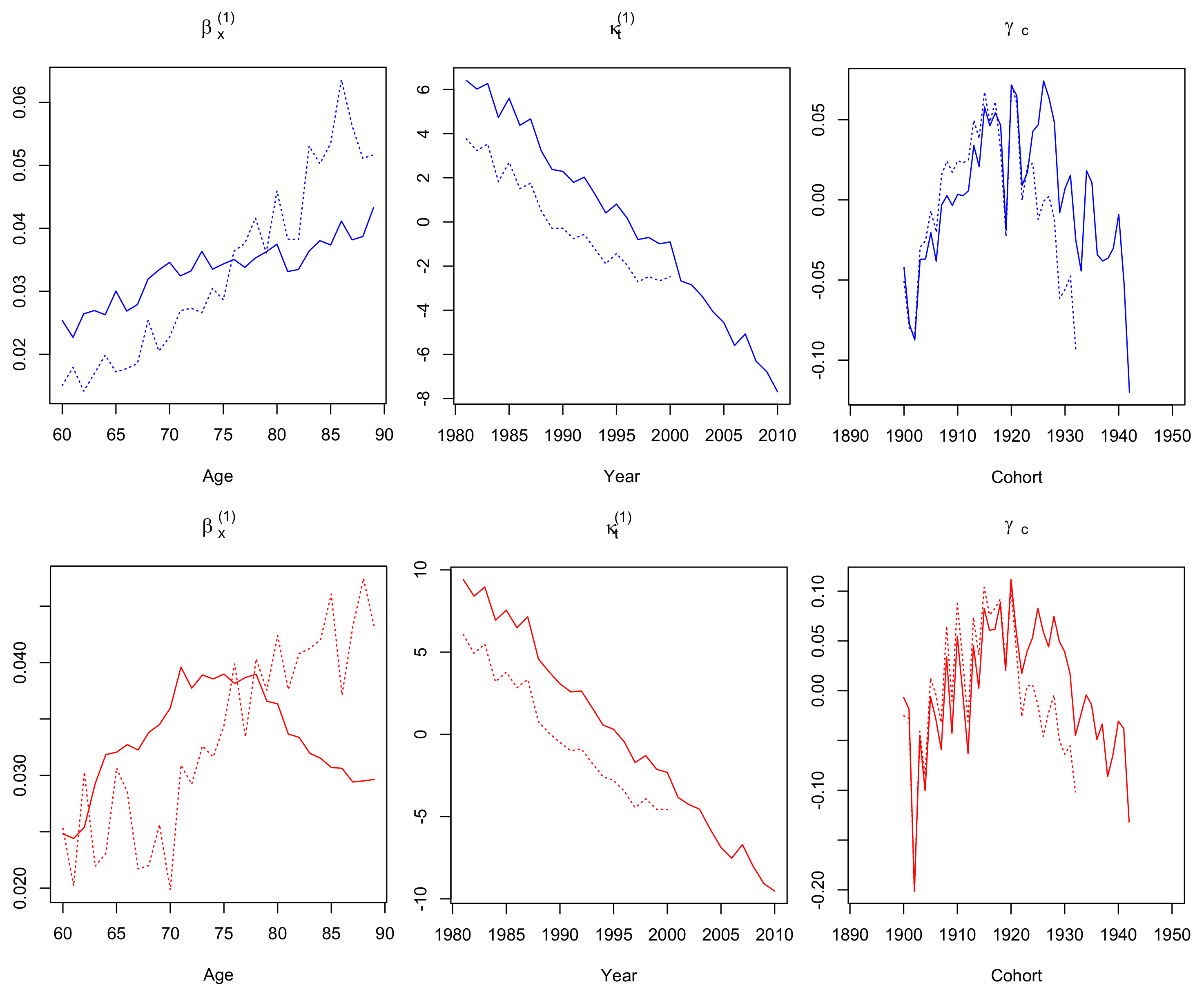
It is worth mentioning that when we firstly fitted ${\displaystyle M2}$ to Greek female data, ${\displaystyle {\kappa }_t^{\left(1\right)}}$ showed an upward trend compared to decreasing ${\displaystyle {\gamma }_{t-x}}$ values. This is the result of the well-known identifiability issues of the Renshaw-Haberman model. To overcome this issue, we considered an additional constraint for the cohort parameter, according to Hunt and Villegas (2015, p. 185). We also note that fitting models ${\displaystyle M_1}$–${\displaystyle M_4}$ under the Poisson assumption (${\displaystyle {\eta }_{x,t}=log{\mu }_{x,t}}$), as they were firstly adjusted in original papers, gave us similar parameter estimates. In addition, robustness of parameter estimates was examined by using two different fitting periods of data: 1981–2010 and 1981–2010. Figure 1, Figure 2, Figure 3, Figure 4, Figure 5, Figure 6 and Figure 7 illustrate the maximum likelihood estimates under the Binomial assumption for models ${\displaystyle M_1}$–${\displaystyle M_7}$ respectively, for Greek males and females, aged 60–89. Solid lines correspond to parameter estimates for the fitting period 1981–2010, while dotted lines for the period 1981–2000. In the following, we give some explanatory comments on parameter estimates.

3.1. Parameter Estimates

The ${\displaystyle {\alpha }_x}$ estimates (Figure 1) show an almost linear upward trend for both genders, which is similar for models ${\displaystyle M_2}$–${\displaystyle M_4}$, therefore it is omitted from Figure 2, Figure 3 and Figure 4. The estimates for ${\displaystyle {\kappa }_t^{\left(1\right)}}$ decrease in every mortality model, indicating a general mortality improvement for both genders over the time. For each one of the (five) models that incorporate a cohort parameter, estimates cannot be safely interpreted as they depend on the whole model setting, including possible interactions with ${\displaystyle {\kappa }_t^{\left(2\right)}}$, ${\displaystyle {\kappa }_t^{\left(3\right)}}$ parameters and the corresponding age effects. More precisely, cohort estimates of ${\displaystyle M_2}$ (Figure 2), ${\displaystyle M_3}$ (Figure 3), ${\displaystyle M_6}$ (Figure 6) and ${\displaystyle M_7}$ (Figure 7) show an increase until year 1915 and decreasing fluctuations for the rest of the cohort years, while ${\displaystyle M_4}$ cohort estimates (Figure 4) fluctuate over the entire period.

Robustness

As Cairns et al. (2009) pointed out, an important property of a model is the robustness of its parameter estimates relative to changes in the range of fitted data. That is, parameter estimates should not change significantly when fitting to a shorter data range. Consequently, a possible lack of robustness for a model means that is sensitive to changes in the period of fitted data and brings into question the appropriateness of its use for projections or other relevant applications that wholly rely on them.

Dotted lines in Figure 1, Figure 2, Figure 3, Figure 4, Figure 5, Figure 6 and Figure 7 indicate that none of the seven models suffers from serious robustness issues. However, use of a fitting range with less data results to an abrupt increase of ${\displaystyle {\beta }_x^{\left(1\right)}}$ female estimates (bottom-left panel of Figure 2) and that remains unchanged even if we repeated model fit, considering less cohorts to be excluded. On the contrary, models ${\displaystyle M_5}$ (Figure 5) and ${\displaystyle M_6}$ (Figure 6) seem to be the most robust ones for both genders.

3.2. Goodness of Fit Diagnostics

A model’s goodness of fit is measured by the scaled residual deviance between the observed and the fitted data, which depends on the chosen distributional assumption. As discussed in Pitacco et al. (2009), lack of randomness in the residuals patterns indicates the inability of a model to capture specific age, period or cohort effects. Under the Binomial distribution assumption of deaths, residual deviance for each model is defined by (Debón et al. 2010, p. 330):

$$D(d_{x,t},{\widehat{d}}_{x,t})=\sum _{x,t}dev(x,t)=\sum _{x,t}2{\omega }_{x,t}\left\{d_{x,t}log\left(\frac{d_{x,t}}{{\widehat{d}}_{x,t}}\right)+(E_{x,t}^0-d_{x,t})log\left(\frac{E_{x,t}^0-d_{x,t}}{E_{x,t}^0-{\widehat{d}}_{x,t}}\right)\right\}.$$

(5)

Then, standardised deviance is given by (Pitacco et al. 2009, p. 254):

$$r_{x,t}=sign(d_{x,t}-{\widehat{d}}_{x,t}){\left(\frac{dev(x,t)}{\widehat{\varphi }}\right)}^{1/2}.$$

(6)

The weights ${\displaystyle {\omega }_{x,t}}$ in Equation (5) are defined as in (4), while ${\displaystyle \widehat{\varphi }=\frac{D(d_{x,t},{\widehat{d}}_{x,t})}{\nu }}$, where ${\displaystyle \nu }$ expresses the degrees of freedom of the model (the number of the observations minus the number of the model parameters).

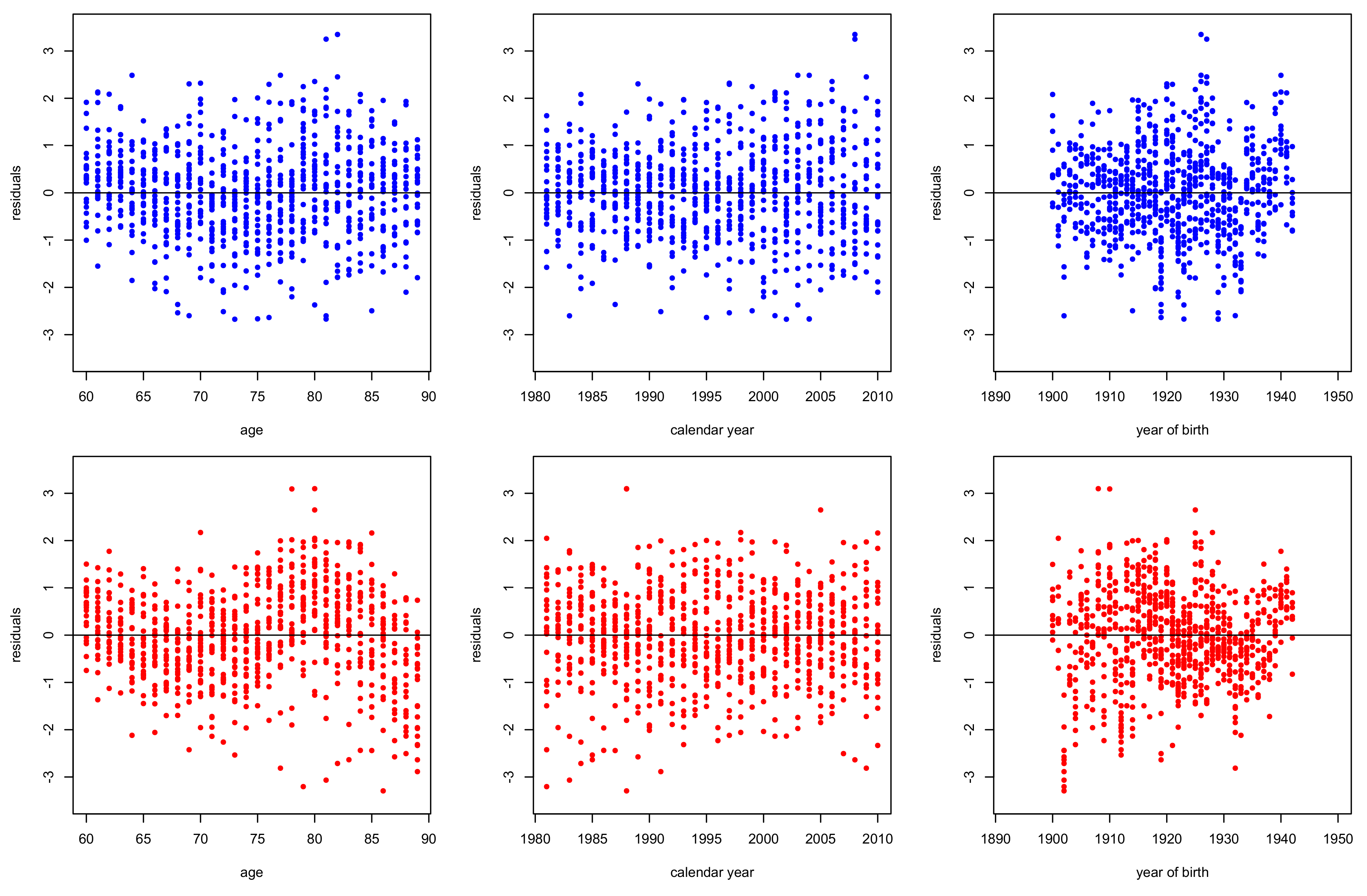
Figure 8, Figure 9, Figure 10, Figure 11, Figure 12, Figure 13 and Figure 14 plot the residuals deviance against age, period (calendar year) and cohort (year of birth) for models ${\displaystyle M_1}$–${\displaystyle M_7}$, fitted for ages 60–89 of period 1981–2010 for males and females. According to the structural features of each model, we can make some comments. The evident dispersion of residuals in the right panels of Figure 8 and Figure 12 reveal the inability of models ${\displaystyle M_1}$ and ${\displaystyle M_5}$, respectively to capture the cohort effect. Moreover, strong patterns in left panels of Figure 12 and Figure 13 illustrate the weakness of models ${\displaystyle M_5}$ and ${\displaystyle M_6}$ respectively to capture the age effects, especially for females. Nonetheless, all the models capture effectively period effects.

3.2.1. Information Criteria

Generally, a better fit is expected from models with more parameters. According to Haberman and Renshaw (2011), an alternative way to address this conjecture is to penalize the model parameters using AIC (Akaike 1974) and BIC (Schwarz 1978) information criteria for each model. In addition, Hurvich and Tsai (1989) derived a correction of the Akaike criterion, the AIC(c), which is more suitable for small samples. Therefore, we use AIC, AIC(c) and BIC, which are defined for model ${\displaystyle M_i,i=1,\cdots ,7}$ as:

$$AI{C}_i\left(c\right)=AI{C}_i+\frac{2k_i(k_i+1)}{n-k_i-1},\mathrm{with}AI{C}_i=2k_i-2log\widehat{L_i}\mathrm{and}$$

$$BI{C}_i=(logn)k_i-2log\widehat{L_i},$$

where ${\displaystyle \widehat{L_i}}$ is the maximum likelihood estimate, ${\displaystyle k_i}$ is the number of the effective parameters5 estimated by ${\displaystyle M_i}$ and ${\displaystyle n}$ is the number of the observations. Smaller AIC, AIC(c) and BIC values indicate a better model fitting.

Table 2. The maximum log likelihood and the number of the effective parameters along with AIC(c), AIC and BIC values (ranking order in brackets) of the mortality models for males and females.

Males
Model	Maximum Log Likelihood	Effective Parameters	AIC	AIC(c)	BIC
${\displaystyle M_1}$	${\displaystyle -}$4487.643	88	9151.287(7)	9172.483(7)	9566.560(7)
${\displaystyle M_2}$	${\displaystyle -}$4191.779	129	8641.558(4)	8689.610(4)	9250.311(4)
${\displaystyle M_3}$	${\displaystyle -}$4218.961	100	8637.922(3)	8665.708(3)	9109.823(2)
${\displaystyle M_4}$	${\displaystyle -}$4202.953	128	8661.907(5)	8709.151(5)	9265.940(5)
${\displaystyle M_5}$	${\displaystyle -}$4501.146	60	9122.291(6)	9131.835(6)	9405.432(6)
${\displaystyle M_6}$	${\displaystyle -}$4209.024	101	8620.048(2)	8648.429(2)	9096.669(1)
${\displaystyle M_7}$	${\displaystyle -}$4160.547	130	8581.094(1)	8629.960(1)	9194.565(3)
Females
${\displaystyle M_1}$	${\displaystyle -}$4980.632	88	10,137.265(6)	10,158.461(6)	10,552.538(6)
${\displaystyle M_2}$	${\displaystyle -}$4254.321	129	8766.643(3)	8814.694(3)	9375.395(3)
${\displaystyle M_3}$	${\displaystyle -}$4367.542	100	8935.085(4)	8962.870(4)	9406.986(4)
${\displaystyle M_4}$	${\displaystyle -}$4235.015	128	8726.030(2)	8773.275(2)	9330.064(2)
${\displaystyle M_5}$	${\displaystyle -}$5279.019	60	10,678.038(7)	10,687.581(7)	10,961.178(7)
${\displaystyle M_6}$	${\displaystyle -}$4474.985	101	9151.969(5)	9180.349(5)	9628.590(5)
${\displaystyle M_7}$	${\displaystyle -}$4209.487	130	8678.975(1)	8727.841(1)	9292.447(1)

presents maximum log likelihood estimates along with the number of the effective parameters and the corresponding AIC, AIC(c) and BIC values of ${\displaystyle M_1}$–${\displaystyle M_7}$ (ranking order in brackets), for males and females.

In line with BIC male results, ${\displaystyle M_6}$ is on top, ${\displaystyle M_3}$ follows and ${\displaystyle M_7}$ is third, while AIC and AIC(c) male rankings coincide, with ${\displaystyle M_7}$, ${\displaystyle M_6}$, ${\displaystyle M_3}$ being on top. Note that BIC penalizes model parameters stronger than AIC and AIC(c), we therefore expect to rank better models containing less parameters. For females, all information criteria coincide to ${\displaystyle M_7}$, ${\displaystyle M_4}$ and ${\displaystyle M_2}$ rank order. Unsurprisingly, ${\displaystyle M_1}$ and ${\displaystyle M_5}$ models hold the worst criteria ranking for both genders, indicating that cohort effect must be taken into account in Greek male and female mortality modelling.

3.2.2. Likelihood-Ratio Test

In Table 1, we can easily observe that some models are special cases of others. More specifically models ${\displaystyle M_1}$ and ${\displaystyle M_3}$ are nested within ${\displaystyle M_2}$, ${\displaystyle M_3}$ in ${\displaystyle M_4}$, ${\displaystyle M_5}$ nests in ${\displaystyle M_6}$ and ${\displaystyle M_7}$ and finally, ${\displaystyle M_6}$ is nested within ${\displaystyle M_7}$. In order to test the null hypothesis that the nested model is the correct versus the alternative hypothesis that the more general is correct, we follow Cairns et al. (2009) in using the Likelihood Ratio (LR) test . Six pairs of tested models and their statistics are presented for both genders in

Table 3. Likelihood ratio test statistics for pairs of nested models (${\displaystyle H_0}$) within general models (${\displaystyle H_1}$).

Males
${\displaystyle {\mathit{H}}_{\mathbf{0}}}$: Nested Model	${\displaystyle {\mathit{H}}_{\mathbf{1}}}$: General Model	Likelihood Ratio Test Statistic	Degrees of Freedom	${\displaystyle \mathit{p}}$-Value
${\displaystyle M_1}$	${\displaystyle M_2}$	591.730	41	${\displaystyle <}$0.0001
${\displaystyle M_3}$	${\displaystyle M_2}$	54.364	29	${\displaystyle <}$0.0001
${\displaystyle M_3}$	${\displaystyle M_4}$	32.015	28	${\displaystyle <}$0.0001
${\displaystyle M_5}$	${\displaystyle M_6}$	584.240	41	${\displaystyle <}$0.0001
${\displaystyle M_5}$	${\displaystyle M_7}$	681.200	70	${\displaystyle <}$0.0001
${\displaystyle M_6}$	${\displaystyle M_7}$	96.955	29	${\displaystyle <}$0.0001
Females
${\displaystyle M_1}$	${\displaystyle M_2}$	1452.600	41	${\displaystyle <}$0.0001
${\displaystyle M_3}$	${\displaystyle M_2}$	226.440	29	${\displaystyle <}$0.0001
${\displaystyle M_3}$	${\displaystyle M_4}$	265.050	28	${\displaystyle <}$0.0001
${\displaystyle M_5}$	${\displaystyle M_6}$	1608.100	41	${\displaystyle <}$0.0001
${\displaystyle M_5}$	${\displaystyle M_7}$	2139.100	70	${\displaystyle <}$0.0001
${\displaystyle M_6}$	${\displaystyle M_7}$	530.990	29	${\displaystyle <}$0.0001

. LR statistic is given by ${\displaystyle {\psi }^{LR}=2log\frac{{\widehat{L}}_2}{{\widehat{L}}_1},}$ where ${\displaystyle {\widehat{L}}_2}$ is the maximum likelihood estimate of the general model and ${\displaystyle {\widehat{L}}_1}$ of the nested model, while ${\displaystyle {\psi }^{LR}}$ approximates a ${\displaystyle {\chi }^2}$ distribution, with ${\displaystyle n_2}$ ${\displaystyle -}$ ${\displaystyle n_1}$ degrees of freedom, where ${\displaystyle n_2}$ are the degrees of the general model and ${\displaystyle n_1}$ of the nested model. For each pair of models in Table 3, null hypothesis is rejected in a significance level ${\displaystyle \alpha }$, since ${\displaystyle {\psi }^{LR}}$ ${\displaystyle >}$ ${\displaystyle {\chi }_{(n_2-n_1),\alpha }^2}$ or the ${\displaystyle p-\mathrm{value}=1-F_{{\chi }_{(n_2-n_1)}^2}\left({\psi }^{LR}\right)}$. Our testing results confirm information criteria rankings, suggesting that models with more parameters fit on Greek data better than more parsimonious models.

4. Mortality Projection

In this section, we estimate future mortality rates using models ${\displaystyle M_1}$–${\displaystyle M_7}$ for both genders. Projection methods are based on the extrapolation of period and cohort parameters for each model fitted on Greek data. Currie (2016) stated that the key point in order to obtain as accurate as possible mortality forecasts is to select the most appropriate time series models that reflect to period and cohort dynamics for a given population. In similar comparative studies, Cairns et al. (2011, p. 357) and Haberman and Renshaw (2011, p. 53) modelled period indices using a multivariate random walk with a drift and cohort indices with univariate ARIMA models.

In our case, we thoroughly selected an appropriate univariate ARIMA model for each period and cohort index over a range of candidate models, according to KPSS (Kwiatkowski et al. 1992), ADF (Dickey and Fuller 1979) and PP (Phillips and Perron 1988) unit root tests and the information criteria values. More precisely, our choice was based on time series overall performance against AIC, AICc and BIC penalized scores. Discordance issues between criteria values were addressed by preferring simpler time series models on grounds of parsimony. Therefore, ${\displaystyle {\kappa }_t}$’s in models ${\displaystyle M_2}$, ${\displaystyle M_3}$, ${\displaystyle M_4}$, ${\displaystyle M_6}$ and ${\displaystyle M_7}$ are assumed to be independent of the corresponding ${\displaystyle {\gamma }_c}$’s for each mortality model, following respectively univariate ARIMA(p,d,q) processes of the forms:

$$(1-{\varphi }_{1}L-\cdots -{\varphi }_p{L}^p){(1-L)}^d{\kappa }_t={\delta }_0+(1+{\theta }_{1}L+\cdots +{\theta }_q{L}^q)e_t,$$

(7)

$$(1-{\varphi }_1^{{}^{\prime }}L-\cdots -{\varphi }_p^{{}^{\prime }}{L}^p){(1-L)}^d{\gamma }_c={\delta }_0^{{}^{\prime }}+(1+{\theta }_1^{{}^{\prime }}L+\cdots +{\theta }_q^{{}^{\prime }}{L}^q)e_c^{{}^{\prime }},$$

(8)

where ${\displaystyle L^d}$ is the time lag operator that shifts data ${\displaystyle d}$ periods back, ${\displaystyle {\delta }_0}$ and ${\displaystyle {\delta }_0^{{}^{\prime }}}$ are constant drift parameters, ${\displaystyle {\varphi }_1,\cdots ,{\varphi }_p}$ and ${\displaystyle {\varphi }_1^{{}^{\prime }},\cdots ,{\varphi }_p^{{}^{\prime }}}$ are the autoregressive coefficients with ${\displaystyle {\varphi }_p\ne 0}$, ${\displaystyle {\varphi }_p^{{}^{\prime }}\ne 0}$, while ${\displaystyle {\theta }_1,\cdots ,{\theta }_q}$ and ${\displaystyle {\theta }_1^{{}^{\prime }},\cdots ,{\theta }_q^{{}^{\prime }}}$ are the moving average parameters with ${\displaystyle {\theta }_q\ne 0}$, ${\displaystyle {\theta }_q^{{}^{\prime }}\ne 0}$ and ${\displaystyle e_t}$, ${\displaystyle e_c^{{}^{\prime }}}$ are white noise processes.

Table 4. Selected ARIMA(p,d,q) models for the period index ${\displaystyle {\kappa }_t^{\left(i\right)},i=1,2,3}$ of male and female mortality models.

Males
Model	${\displaystyle {\mathit{\kappa }}_{\mathit{t}}^{\left(\mathbf{1}\right)}}$	${\displaystyle {\mathit{\kappa }}_{\mathit{t}}^{\left(\mathbf{2}\right)}}$	${\displaystyle {\mathit{\kappa }}_{\mathit{t}}^{\left(\mathbf{3}\right)}}$
${\displaystyle M_1}$	ARIMA(0,2,2)	—–	—–
${\displaystyle M_2}$	ARIMA(0,1,1) with drift	—–	—–
${\displaystyle M_3}$	ARIMA(1,1,0) with drift	—–	—–
${\displaystyle M_4}$	ARIMA(0,2,2)	ARIMA(2,1,0) with drift	—–
${\displaystyle M_5}$	ARIMA(1,2,1)	ARIMA(2,1,0) with drift	—–
${\displaystyle M_6}$	ARIMA(0,2,2) with drift	ARIMA(0,1,1) with drift	—–
${\displaystyle M_7}$	ARIMA(1,2,1)	ARIMA(2,2,0)	ARIMA(0,1,1) with drift
Females
Model	${\displaystyle {\mathit{\kappa }}_{\mathit{t}}^{\left(\mathbf{1}\right)}}$	${\displaystyle {\mathit{\kappa }}_{\mathit{t}}^{\left(\mathbf{2}\right)}}$	${\displaystyle {\mathit{\kappa }}_{\mathit{t}}^{\left(\mathbf{3}\right)}}$
${\displaystyle M_1}$	ARIMA(1,1,0) with drift	—–	—–
${\displaystyle M_2}$	ARIMA(3,1,0) with drift	—–	—–
${\displaystyle M_3}$	ARIMA(3,1,0) with drift	—–	—–
${\displaystyle M_4}$	ARIMA(1,1,0) with drift	ARIMA(1,1,0) with drift	—–
${\displaystyle M_5}$	ARIMA(0,2,2)	ARIMA(0,1,0) with drift	—–
${\displaystyle M_6}$	ARIMA(0,1,1) with drift	ARIMA(0,1,1) with drift	—–
${\displaystyle M_7}$	ARIMA(2,1,0) with drift	ARIMA(2,2,0)	ARIMA(0,1,1) with drift

and

Table 5. Selected ARIMA(p,d,q) models for the cohort index ${\displaystyle {\gamma }_c}$ of male and female mortality models.

Model	${\displaystyle {\mathit{\gamma }}_{\mathit{c}}}$ for Males	${\displaystyle {\mathit{\gamma }}_{\mathit{c}}}$ for Females
${\displaystyle M_2}$	ARIMA(2,1,0)	ARIMA(2,1,1) with drift
${\displaystyle M_3}$	ARIMA(0,0,1)	ARIMA(4,1,1)
${\displaystyle M_4}$	ARIMA(0,0,2)	ARIMA(4,1,1)
${\displaystyle M_6}$	ARIMA(0,1,3)	ARIMA(3,0,2)
${\displaystyle M_7}$	ARIMA(0,0,1)	ARIMA(4,0,1)

present the selected ARIMA models for period and cohort indices, respectively for males and females. For all models period indices are assumed to be modelled independently. Also remind that ${\displaystyle M_1}$ and ${\displaystyle M_5}$ do not incorporate a cohort index.

Time series Equations (7) and (8) were simulated to produce 1000 trajectories for future values of the period ${\displaystyle {\widehat{\kappa }}_{t_n+s}}$ and the cohort ${\displaystyle {\widehat{\gamma }}_{t_n+s-x}}$ indices, where ${\displaystyle s=1,2,\cdots ,20}$ denotes the years of the forecasting horizon. Then, future simulated mortality values are extracted using:

$$\widehat{\mathrm{logit}{q}_{x,t_n+s}}={\alpha }_x+\sum _{i=1}^N{\beta }_x^{\left(i\right)}{\widehat{\kappa }}_{t_n+s}^{\left(i\right)}+{\widehat{\gamma }}_{t_n+s-x},$$

or

$${\widehat{q}}_{x,t_n+s}=\frac{exp({\alpha }_x+{\sum }_{i=1}^N{\beta }_x^{\left(i\right)}{\widehat{\kappa }}_{t_n+s}^{\left(i\right)}+{\widehat{\gamma }}_{t_n+s-x})}{1+exp({\alpha }_x+{\sum }_{i=1}^N{\beta }_x^{\left(i\right)}{\widehat{\kappa }}_{t_n+s}^{\left(i\right)}+{\widehat{\gamma }}_{t_n+s-x})},$$

(9)

where ${\displaystyle t_n=2010}$ is the last year of the fitting period and ${\displaystyle \mathrm{logit}{\widehat{q}}_{x,t_n+s}}$ denotes the logit-transform of future probabilities of death for each age ${\displaystyle x}$ for models ${\displaystyle M_1}$–${\displaystyle M_7}$.

Then, the predictive power of mortality models was evaluated by measuring the differences (errors) between the observed and the forecasted values for the same period. For the first three out-of-sample years of projection (${\displaystyle t_n=2010,s=1,2,3}$), in which Greek mortality data are available in HMD, forecast accuracy of models ${\displaystyle M_1}$–${\displaystyle M_7}$ can be evaluated by averaging the mean absolute error (MAE) and the mean absolute percentage error (MAPE) values over the 3-years period for ages ${\displaystyle 60}$ to ${\displaystyle 89}$, using Equations (10) and (11), respectively.

$$MA{E}_{avg}=\frac{1}{3\times (89-60+1)}\sum _{s=1}^3\sum _{x=60}^{89}\left|{\widehat{q}}_{x,2010+s}-q_{x,2010+s}\right|\times 100,$$

(10)

$$MAP{E}_{avg}=\frac{1}{3\times (89-60+1)}\sum _{s=1}^3\sum _{x=60}^{89}\left|\frac{{\widehat{q}}_{x,2010+s}-q_{x,2010+s}}{q_{x,2010+s}}\right|.$$

(11)

Short-term male and female forecast errors of period 2011–2013 were extracted for models ${\displaystyle M_1}$–${\displaystyle M_7}$, while for the sake of comparison, extrapolation was firstly performed by using fitted jump-off rates6 and secondly by using actual rates for the year 2010 (

Table 6. Averaged values (ranking order in brackets) of the mean absolute error (MAE) and mean absolute percentage error (MAPE) measures of the forecasting period 2011–2013 using fitted or actual jump-off rates for males and females.

Fitted Jump-off Rates
Males
Error	${\displaystyle M_1}$	${\displaystyle M_2}$	${\displaystyle M_3}$	${\displaystyle M_4}$	${\displaystyle M_5}$	${\displaystyle M_6}$	${\displaystyle M_7}$
${\displaystyle MA{E}_{avg}}$	0.332(6)	0.251(1)	0.253(2)	0.287(3)	0.327(5)	0.295(4)	0.346(7)
${\displaystyle MAP{E}_{avg}}$	10.194(4)	6.496(1)	6.583(2)	9.385(3)	10.935(6)	10.559(5)	15.697(7)
Females
${\displaystyle MA{E}_{avg}}$	0.207(4)	0.147(1)	0.165(2)	0.219(5)	0.234(6)	0.198(3)	0.281(7)
${\displaystyle MAP{E}_{avg}}$	10.363(3)	6.052(1)	7.981(2)	12.239(5)	13.396(6)	11.216(4)	22.340(7)
Actual Jump-off Rates
Males
Error	${\displaystyle M_1}$	${\displaystyle M_2}$	${\displaystyle M_3}$	${\displaystyle M_4}$	${\displaystyle M_5}$	${\displaystyle M_6}$	${\displaystyle M_7}$
${\displaystyle MA{E}_{avg}}$	0.273(6)	0.213(3)	0.208(2)	0.192(1)	0.289(7)	0.237(4)	0.247(5)
${\displaystyle MAP{E}_{avg}}$	6.780(5)	5.222(2)	5.086(1)	5.371(3)	6.916(6)	6.020(4)	8.545(7)
Females
${\displaystyle MA{E}_{avg}}$	0.213(6)	0.180(3)	0.168(2)	0.196(4)	0.200(5)	0.165(1)	0.250(7)
${\displaystyle MAP{E}_{avg}}$	7.073(5)	5.570(2)	5.336(1)	6.225(4)	7.283(6)	5.866(3)	11.818(7)

), taken directly from HMD. Measures show that models ${\displaystyle M_2}$, ${\displaystyle M_3}$, ${\displaystyle M_4}$ and ${\displaystyle M_6}$ produce better forecasts for both genders (ranking order in brackets), either by using fitted or actual jump-off rates. Especially, when fitted rates are used, models ${\displaystyle M_2}$ and ${\displaystyle M_3}$ distinguish for both genders, while for actual rates M4 and M3 are dominant for males and ${\displaystyle M_6}$ outperforms for females. In any case, both of the three error measures give the higher error values for ${\displaystyle M_1}$, ${\displaystyle M_5}$ and ${\displaystyle M_7}$, indicating the presence of cohort effects in male and female mortality indices that cannot be captured by models ${\displaystyle M_1}$, ${\displaystyle M_5}$ and a possible overfitting behaviour of ${\displaystyle M_7}$.

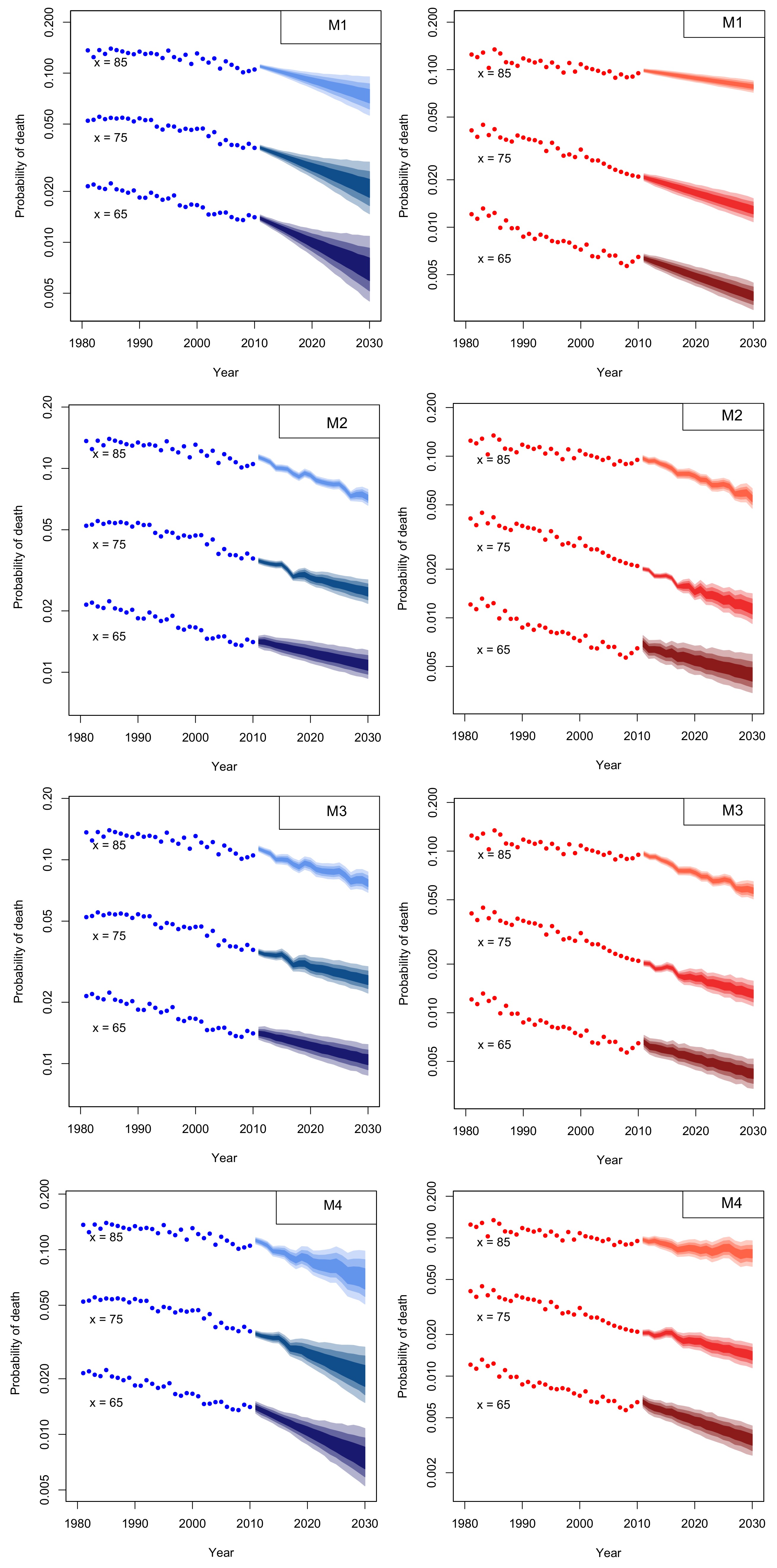
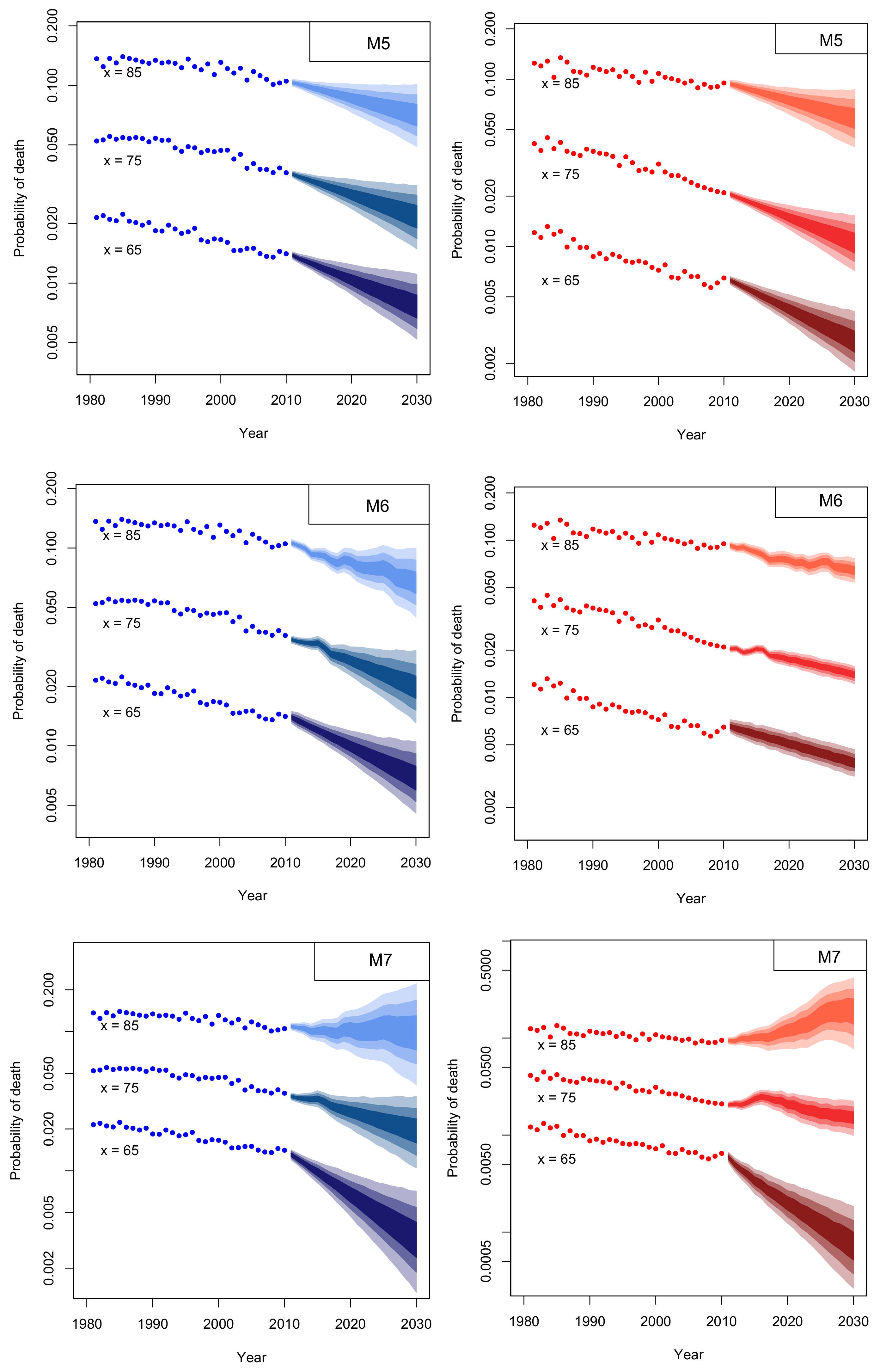
Long-term mortality projections for a 20 year horizon ahead were obtained using (9) with actual jump-off rates for the seven mortality models, incorporating 1000 simulation trajectories of the selected period and cohort indices. The simulated one year probabilities of death (in logarithmic scale) for models ${\displaystyle M_1}$–${\displaystyle M_7}$ are illustrated for both genders in Figure 15.

Plotting results reveal the appropriateness of a mortality model for long-term forecasting. In addition, according to Cairns et al. (2011); Villegas et al. (2017) differences in uncertainty levels of each model indicates the significance of model risk in mortality forecasting.

Figure 15 shows that ${\displaystyle M_1}$, ${\displaystyle M_2}$ and ${\displaystyle M_3}$ forecasts seem to be implausible for both genders, since fans at age 85 are notably narrower than at age 65. Furthermore, ${\displaystyle M_4}$ and ${\displaystyle M_6}$ fans at age 75 show a weak, but not significant increase for both genders, while fans at age 85 show some decreasing fluctuations. On the other hand, parsimonious model ${\displaystyle M_5}$ performs well in general for both genders. Finally, female fans of model ${\displaystyle M_7}$ are narrower age 75 and 85 than at 65 and show an unreasonable increase in older ages. This is mainly because forecasts are linked to the estimated cohort effect of Figure 7 that exhibits a steep, upward and linear trend between cohort years 1930 and 1940.

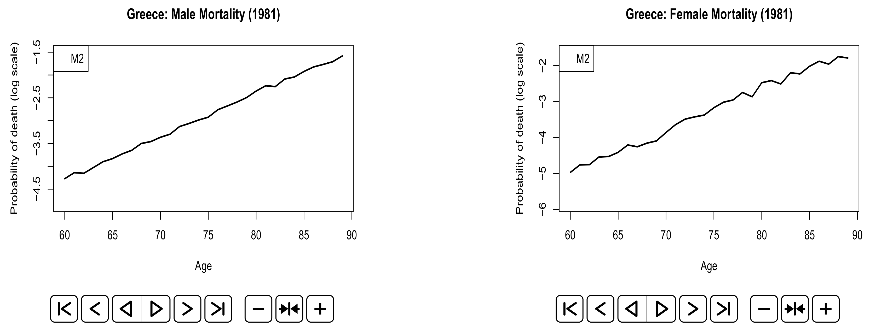
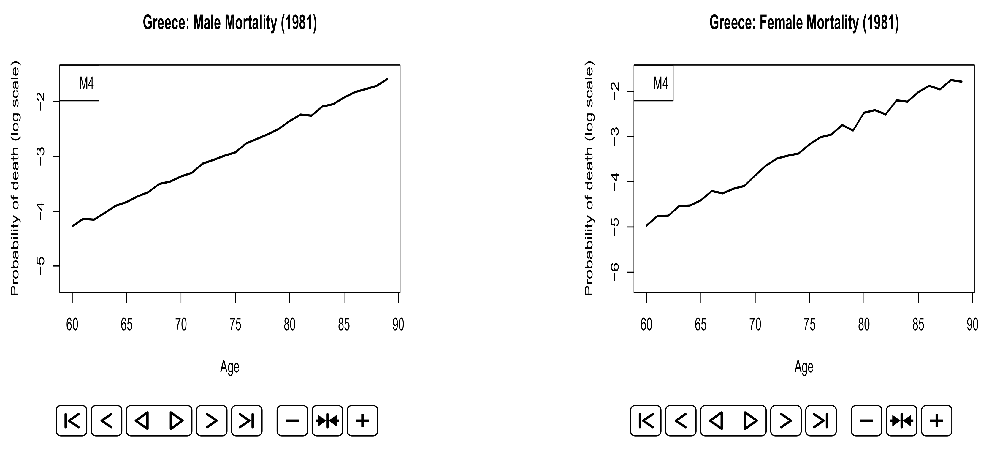
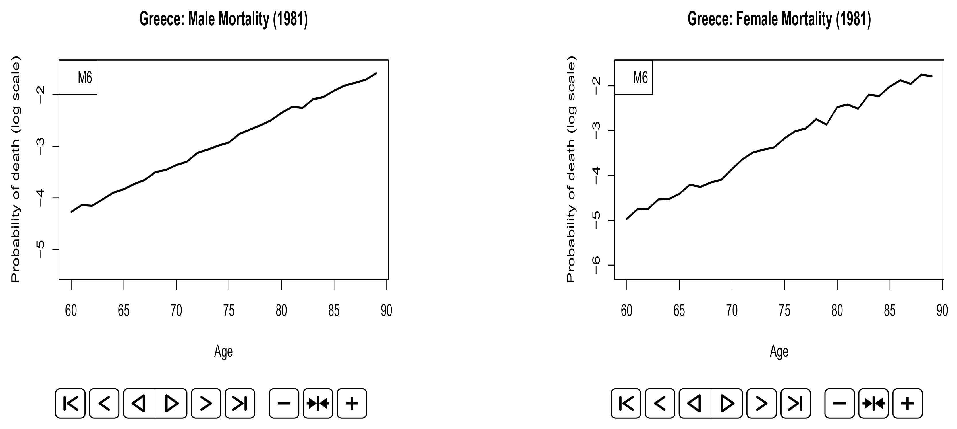
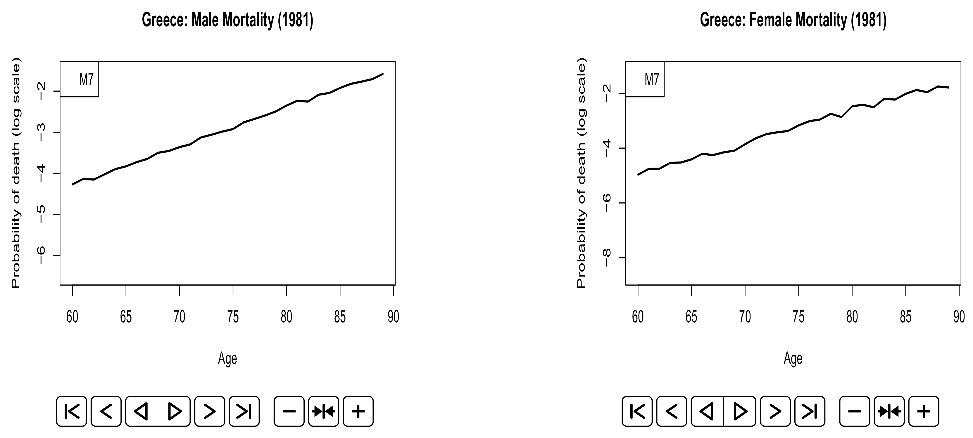
Animated figures of the overall evolution of death rates for each model are also given in Figure A1, Figure A2, Figure A3, Figure A4, Figure A5, Figure A6 and Figure A7 of Appendix A, as an alternative, more interactive way to present our results. Animated figures were created using the “animation” R-package (Xie 2013).

4.1. Assessing Parameter Risk

We observe that mortality projections obtained with stochastic models incorporate only the forecast error that arises from the estimation of the period and the cohort indices, ignoring the effects of the so called parameter risk. Especially, for countries with limited data experience such as Greece, use of bootstrapping techniques is required to address this issue. Therefore, we exploit the advantages of a residual bootstrapping method to assess the parameter uncertainty in mortality projections for the seven models, described in the previous sections.

In their study, Renshaw and Haberman (2008) proposed a residual bootstrapped method to accommodate uncertainty in estimating the parameters of the Lee-Carter model under the Poisson assumption of deaths. In our case, we produce bootstrap samples under the Binomial distribution assumption, following a slightly modified approach described by Debón et al. (2010, p. 330).

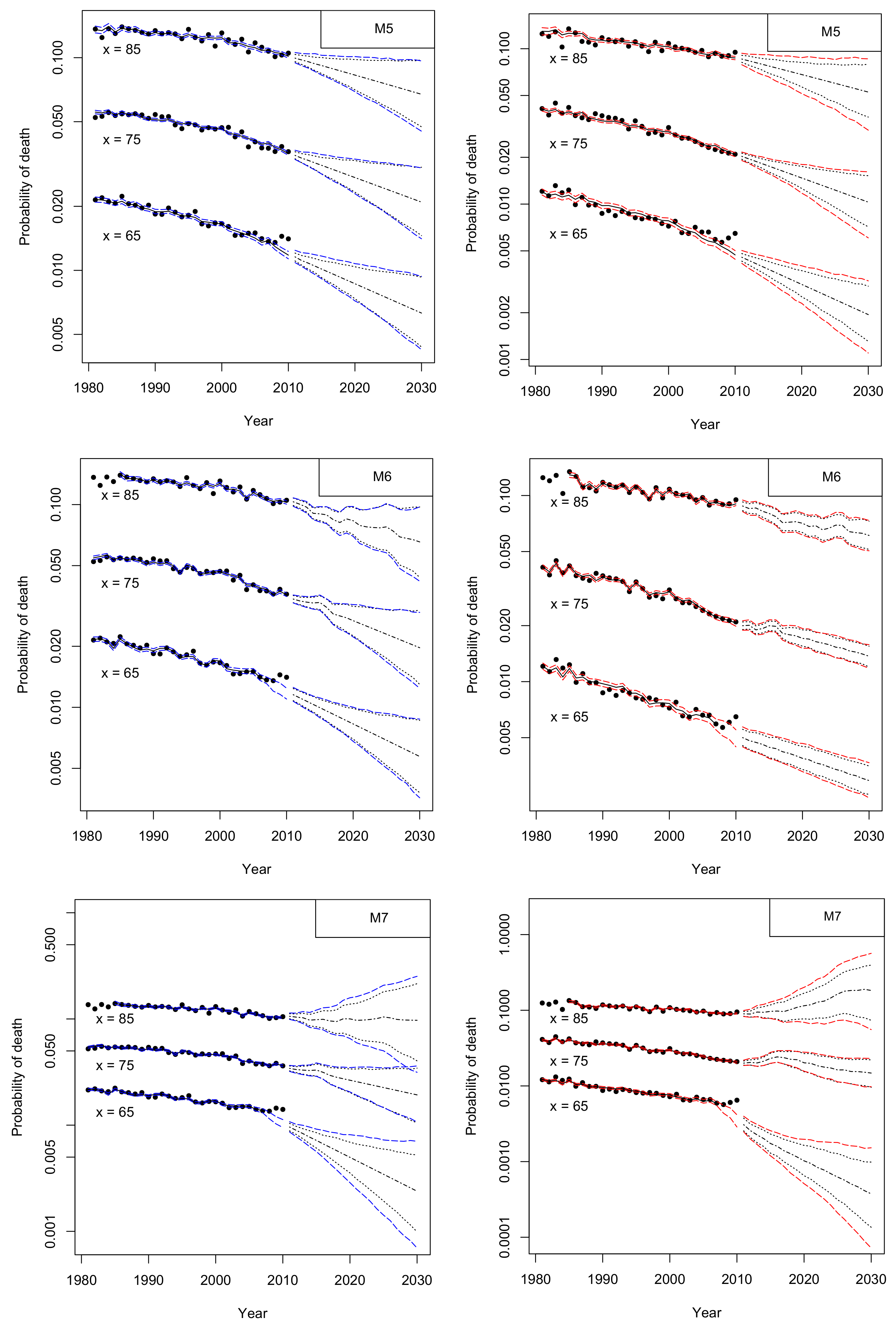
Simulations were carried out using “StMoMo” R-package and 1000 trajectories were generated to compare the prediction intervals of the forecast error and the parameter estimation uncertainty of projections. Figure 16 illustrates for both genders the 95% prediction intervals for the probabilities of death at ages ${\displaystyle x=65}$, ${\displaystyle x=75}$ and ${\displaystyle x=85}$ for models ${\displaystyle M_1}$–${\displaystyle M_7}$, fitted to Greek data for ages 60–89 of the period 1981–2010. Historical rates are denoted by thick dots, solid lines denote the corresponding fitted rates and dot-dashed lines depict the 95% confidence intervals including parameter uncertainty. For the projection period 2011–2030, dashed lines represent the central forecast values and dot lines show the 95% prediction intervals excluding parameter uncertainty. The dot-dashed lines depict the 95% prediction intervals accounting for parameter uncertainty.

Figure 16 shows an evident parameter uncertainty in the projection period for males (left panels) of models ${\displaystyle M_2}$ (age 85) and ${\displaystyle M_7}$ (ages 65 and 85). Parameter variability is also observed for females of the same models (right panels), with an implausible upward trend for ${\displaystyle M_7}$ at age 75 and 85, which indicates the inappropriateness of this model to forecast female mortality at higher ages.

4.2. Application in Insurance-Related Products

An appropriate mortality modelling method constitutes an essential tool in pricing insurance products. In addition, as Lovász (2011) point out, insurance-related application results reflect the appropriateness of a model choice. In the following, we apply the cohort mortality forecasts obtained from ${\displaystyle M_1}$–${\displaystyle M_7}$ to calculate life insurance premiums, similarly as in Tsai and Lin (2016, p. 16). Let us denote as ${\displaystyle A_{\stackrel{1}{x},t_n+1:\overline{K\hspace{.2em}|}}}$ the fully discrete life insurance premium issued to an insured aged ${\displaystyle x}$ in year ${\displaystyle t_n+1}$, payable at the end of the year of death, if it occurs within a term of ${\displaystyle K}$ years and as ${\displaystyle A_{x,t_n+1:\stackrel{1}{\overline{K\hspace{.2em}|}}}}$ the pure endowment issued to an insured aged ${\displaystyle x}$ in year ${\displaystyle t_n+1}$, payable at the end of ${\displaystyle K}$ years in case of being alive. Net premiums (NP) are given respectively by:

$$A_{\stackrel{1}{x},t_n+1:\overline{K\hspace{.2em}|}}=\sum _{k=0}^{K-1}{}_k{p}_{x,t_n+1}·q_{x+k,t_n+1+k}·{(1+i)}^{-(k+1)},$$

(12)

$$A_{x,t_n+1:\stackrel{1}{\overline{K\hspace{.2em}|}}}={}_K{p}_{x,t_n+1}·{(1+i)}^{-K},$$

(13)

where ${\displaystyle {}_k{p}_{x,t_n+1}}$ denotes the k-year survival probability for age ${\displaystyle x}$ in year ${\displaystyle t_n+1}$, while its estimate is given by ${\displaystyle {}_k{\widehat{p}}_{x,t_n+1}={\widehat{p}}_{x,t_n+1}.....{\widehat{p}}_{x+k-1,t_n+1+k-1}}$, ${\displaystyle k=1,\cdots ,K-1}$ (similarly for ${\displaystyle {}_K{\widehat{p}}_{x,t_n+1}}$), ${\displaystyle i}$ is the interest rate and ${\displaystyle {}_0{\widehat{p}}_{x,t_n+1}=1}$.

Since mortality projection models are typically used for pension applications, it would also be beneficial to see the performance of a life annuity product. Let us denote as ${\displaystyle {\ddot{a}}_{x,t_n+1:\overline{K\hspace{.2em}|}}}$ a discrete life annuity-due of an insured aged ${\displaystyle x}$ in year ${\displaystyle t_n+1}$, payable on an annual basis for up to ${\displaystyle K}$ years, so long as insured survives. Actuarial present value (APV) is given by:

$${\ddot{a}}_{x,t_n+1:\overline{K\hspace{.2em}|}}=\sum _{k=0}^{K-1}{}_k{p}_{x,t_n+1}.{(1+i)}^{-k}.$$

(14)

Hence, we apply the estimated mortality rates obtained from ${\displaystyle M_1}$–${\displaystyle M_7}$, fitted to 1981–2000 with actual jump-off rates to calculate life insurance NPs and annuity APV for ages 60–79 with ${\displaystyle K=10}$, assuming ${\displaystyle i=4\%}$. As before, we use averaged MAE and MAPE to evaluate the errors between forecasted NPs and those produced from the observed mortality rates for the years 2001–2010. For each model, error measures for life insurance premiums are given by:

$$MA{E}_x^{(K=10)}=\frac{1}{20}\sum _{x=60}^{79}\left|{\widehat{A}}_{\stackrel{1}{x},2001:\overline{10\hspace{.2em}|}}-A_{\stackrel{1}{x},2001:\overline{10\hspace{.2em}|}}\right|\times 100,$$

(15)

$$MAP{E}_x^{(K=10)}=\frac{1}{20}\sum _{x=60}^{79}\left|\frac{{\widehat{A}}_{\stackrel{1}{x},2001:\overline{10\hspace{.2em}|}}-A_{\stackrel{1}{x},2001:\overline{10\hspace{.2em}|}}}{A_{\stackrel{1}{x},2001:\overline{10\hspace{.2em}|}}}\right|.$$

(16)

Similarly, MAE and MAPE formulas are adjusted for pure endowment or annuity products by replacing ${\displaystyle A_{\stackrel{1}{x},t_n+1:\overline{K\hspace{.2em}|}}}$ with ${\displaystyle A_{x,t_n+1:\stackrel{1}{\overline{K\hspace{.2em}|}}}}$ or ${\displaystyle {\ddot{a}}_{x,t_n+1:\overline{K\hspace{.2em}|}}}$ in (15) and (16).

Table 7. Averaged values (ranking order in brackets) of MAE and MAPE measures for 10 year forecasted life insurance, pure endowment and life annuity values using actual jump-off rates for males and females, aged 60–79 in 2001–2010.

Life Insurance
Males
Error	${\displaystyle M_1}$	${\displaystyle M_2}$	${\displaystyle M_3}$	${\displaystyle M_4}$	${\displaystyle M_5}$	${\displaystyle M_6}$	${\displaystyle M_7}$
${\displaystyle MA{E}_x}$	2.222(6)	1.242(1)	2.284(7)	2.199(5)	2.020(4)	1.456(2)	1.799(3)
${\displaystyle MAP{E}_x}$	7.651(6)	5.536(1)	8.895(7)	7.626(5)	7.412(4)	5.557(2)	6.490(3)
Females
${\displaystyle MA{E}_x}$	1.605(6)	0.870(1)	0.885(2)	1.494(5)	0.914(3)	1.016(4)	2.150(7)
${\displaystyle MAP{E}_x}$	9.264(5)	6.404(1)	6.901(3)	9.268(6)	6.426(2)	6.930(4)	11.883(7)
Pure Endowment
Males
Error	${\displaystyle M_1}$	${\displaystyle M_2}$	${\displaystyle M_3}$	${\displaystyle M_4}$	${\displaystyle M_5}$	${\displaystyle M_6}$	${\displaystyle M_7}$
${\displaystyle MA{E}_x}$	1.605(6)	0.927(1)	1.666(7)	1.590(5)	1.451(4)	1.039(2)	1.293(3)
${\displaystyle MAP{E}_x}$	4.114(7)	2.190(1)	4.094(6)	4.064(5)	3.619(4)	2.531(2)	3.212(3)
Females
${\displaystyle MA{E}_x}$	1.198(6)	0.623(1)	0.651(2)	1.091(5)	0.690(3)	0.738(4)	1.556(7)
${\displaystyle MAP{E}_x}$	2.615(6)	1.282(2)	1.242(1)	2.250(5)	1.408(3)	1.565(4)	3.240(7)
Life Annuity
Males
Error	${\displaystyle M_1}$	${\displaystyle M_2}$	${\displaystyle M_3}$	${\displaystyle M_4}$	${\displaystyle M_5}$	${\displaystyle M_6}$	${\displaystyle M_7}$
${\displaystyle MA{E}_x}$	7.711(6)	5.506(2)	8.132(7)	7.637(5)	6.781(4)	5.225(1)	5.924(3)
${\displaystyle MAP{E}_x}$	1.127(6)	0.785(2)	1.168(7)	1.112(5)	0.980(4)	0.748(1)	0.856(3)
Females
${\displaystyle MA{E}_x}$	5.484(6)	2.465(1)	2.944(2)	4.995(5)	3.254(4)	3.091(3)	6.466(7)
${\displaystyle MAP{E}_x}$	0.754(6)	0.325(1)	0.386(2)	0.673(5)	0.439(4)	0.416(3)	0.873(7)

presents the averaged values of MAE and MAPE values in ranking order for a 10 year forecasted life insurance, pure endowment and life annuity using actual jump-off rates for males and females, aged 60–79 in 2001–2010, while Figure 17 illustrates the MAE and MAPE values against age for life insurance and annuity products, respectively for males (left panels) and females (right panels) for the top four models in ranking.

According to MAE and MAPE values, models ${\displaystyle M_2}$, ${\displaystyle M_6}$ and ${\displaystyle M_7}$ produce better insurance-related forecasts for males, while ${\displaystyle M_2}$, ${\displaystyle M_3}$ and ${\displaystyle M_5}$ are the top ranked models for females. For both genders, measures show that ${\displaystyle M_2}$ outperforms in aggregate. However, regarding its robustness (especially for female data) and taking into account values of Table 7, a good insurance-related model choice should also be ${\displaystyle M_6}$ for males and ${\displaystyle M_3}$ for females. This fact is also evident in Figure 17, where absolute error and absolute percentage error values against age for the corresponding models lie on the lower levels for both insurance products.

5. Results

In this section, we summarize the fitting and forecasting results of this analysis and our findings are compared with the corresponding results obtained from the original papers. Our study shows that all the models capture effectively the period effects for both genders. We can also notice that the most parsimonious models ${\displaystyle M_1}$ and ${\displaystyle M_5}$ do not capture the cohort effect as it is illustrated in the right panels of male and female scatter plots of residual deviance in Figure 8 and Figure 12. Furthermore, models ${\displaystyle M_5}$ and ${\displaystyle M_6}$ seem to be inadequate to capture the age effects, especially for females (left panels in Figure 12 and Figure 13).

AIC and AIC(c) scores coincide to the fact that models ${\displaystyle M_7}$, ${\displaystyle M_6}$ and ${\displaystyle M_3}$ outperform in ordered ranking for males, while in the BIC rankings7 ${\displaystyle M_6}$ is on top, ${\displaystyle M_3}$ follows and ${\displaystyle M_7}$ is third. For females, all measure values show that ${\displaystyle M_7}$ comes out first, ${\displaystyle M_4}$ second and ${\displaystyle M_2}$ follows. For both genders, models ${\displaystyle M_1}$ and ${\displaystyle M_5}$ have the worst criteria ranking for both genders, lacking a cohort term that must be taken into account in Greek male and female mortality modelling. Likelihood ratio results confirm the information criteria ranking, indicating that the more complicated models ${\displaystyle M2}$, ${\displaystyle M_4}$, ${\displaystyle M_6}$ and ${\displaystyle M_7}$ are in aggregate more suitable for modelling Greek mortality.

Mortality projections derived from the seven models are illustrated for both genders in Figure 15. Plotting results show that long-term forecasts from model ${\displaystyle M_1}$, ${\displaystyle M_2}$ and ${\displaystyle M_3}$ seem to be unreliable for both genders, since figures at age 85 are notably narrower than at age 65. In addition, model ${\displaystyle M_7}$ for females shows an implausible increase of mortality rates at ages 75 and 85. However, forecast accuracy measures of Table 6 suggests that models ${\displaystyle M_2}$, ${\displaystyle M_3}$, ${\displaystyle M_5}$ and ${\displaystyle M_6}$ produce better short-term forecasts for both genders.

Parameter uncertainty is evident in models ${\displaystyle M_2}$ and ${\displaystyle M_7}$ for both genders in higher ages (Figure 16). Parameter variability is also observed in model ${\displaystyle M_5}$ for females, while while the implausible upward trend for ${\displaystyle M_7}$ at age 75 and 85 raise some questions regarding the appropriateness of this model to forecast Greek female mortality.

Comparison with Original Papers

Now we present the commonalities and differences between estimation results of our study and the corresponding findings obtained from the original papers.

Lee and Carter (1992) modelled the mortality rates of the entire United States population for grouped ages ${\displaystyle 0}$–${\displaystyle {85}^{+}}$ of years 1933–1987. The same year, Carter and Lee (1992) implemented their model for males and females separately, using the SVD method to derive forecasts of the ${\displaystyle {\kappa }_t^{\left(1\right)}}$ time index for a full range of grouped ages ${\displaystyle 0}$–${\displaystyle {85}^{+}}$ of the years 1933–1988. Fitted values of ${\displaystyle {\alpha }_x}$ and ${\displaystyle {\beta }_x^{\left(1\right)}}$ for Greek males and females of our study show similar trends with the corresponding results obtained for both genders of the United States population data. Likewise, comparing our estimates with the corresponding Belgian results obtained from the Poisson Lee-Carter approach of Brouhns et al. (2002), we observed that their maximum likelihood estimates of ${\displaystyle {\alpha }_x}$, ${\displaystyle {\beta }_x^{\left(1\right)}}$ and ${\displaystyle {\kappa }_t^{\left(1\right)}}$ for ages 60–98 in the years 1960–1998 are in line with the Greek results, especially for males, where the estimates lie between the same levels.

The Haberman and Renshaw (2011) model estimates obtained from fitting ages 55–89 of years 1961–2007 for England and Wales male data. Even if estimates show similar patterns, they cannot be directly compared with our results, since authors used different model constraints (Haberman and Renshaw 2011, p. 37) in their analysis.

The Currie (2006) model was initially fitted to selected assured lives, aged 20–90, for the years 1947–2002. Estimates of ${\displaystyle {\alpha }_x}$ are in accordance with our results for both genders. The period component of the model shows an upward trend between 1950–1975, but after the year 1980, it complies with Greek patterns.

Plat (2009) fitted his model to three different data sets of males for: the United states (ages 20–84, years 1961–2005), the England and Wales (ages 20–89, years 1961–2005) and the Netherlands (ages 20–90, years 1951–2005). Estimated parameters ${\displaystyle {\alpha }_x}$ and ${\displaystyle {\kappa }_t^{\left(1\right)}}$, ${\displaystyle {\kappa }_t^{\left(2\right)}}$ and ${\displaystyle {\gamma }_{t-x}}$ were illustrated only for the United States mortality data. Although his ${\displaystyle {\alpha }_x}$ and ${\displaystyle {\kappa }_t^{\left(1\right)}}$ male estimates were based on a wide age range of data fitted onto his extended model form, they totally agree with our corresponding values exported from the reduced model form used for Greek data of ages 60–89. In the contrary, ${\displaystyle {\kappa }_t^{\left(2\right)}}$ parameter estimates have completely different trends for the entire common period, while the ${\displaystyle {\gamma }_{t-x}}$ parameter values show similar patterns with the Greek males between cohort years 1890–1930 (Figure 4).

Cairns et al. (2006) illustrated their model using England and Wales data of males, aged 60–90, for the years 1961–2002. Their results show that ${\displaystyle {\kappa }_t^{\left(1\right)}}$ estimated values have a steep downward trend for the whole fitting period, while ${\displaystyle {\kappa }_t^{\left(2\right)}}$ values follow an opposite upward trend for the same years. Estimates of these two parameters are obviously similar with the corresponding Greek results, obtained for ages 60–89 of period 1981–2010. This is more evident for ${\displaystyle {\kappa }_t^{\left(2\right)}}$ parameter, where its values lie between the same levels for both countries.

The Cairns et al. (2009) “cohort” extension of the Cairns et al. (2006) model was fitted to England and Wales (1961–2004) and United States (1968–2003) male data for ages 60–89. ${\displaystyle {\kappa }_t^{\left(1\right)}}$ and ${\displaystyle {\kappa }_t^{\left(2\right)}}$ estimates for England and Wales data are in accordance with the Greek values, showing a decreasing trend for the first parameter and an upward trend for the second one, respectively. Cohort estimates lie between the same levels with the Greek ones, with an exception after birth year 1935, where Greek cohort estimates jump abruptly to higher levels. The corresponding ${\displaystyle {\kappa }_t}$ results for the United States data are quite similar, but the ${\displaystyle {\gamma }_{t-x}}$ parameter estimates show a steep fall around the year 1920 in comparison with the derived Greek results.

The “quadratic” extension of the Cairns et al. (2006) model was illustrated in Cairns et al. (2009) for the England and Wales (1961–2004) and the United States (1968–2003) male data for ages 60–89. Although ${\displaystyle {\kappa }_t^{\left(1\right)}}$, ${\displaystyle {\kappa }_t^{\left(2\right)}}$ and ${\displaystyle {\gamma }_{t-x}}$ estimates for England and Wales and United States males take similar values and show the same patterns with the corresponding Greek population data, some differences are observed in the estimates ${\displaystyle {\kappa }_t^{\left(3\right)}}$, where a steep, upward trend between the years 1985–2003 is evident for both countries in contrast with the decreasing Greek values.

For the sake of comparability, we point out that when van Berkum et al. (2016) analyzed the impact of allowing for multiple structural changes on a large collection of mortality models for Dutch and Belgian male data of ages 60–89 for the period 1950–2008, they reached to similar ranking results with our findings.

6. Concluding Remarks

A comparative analysis of seven stochastic mortality models of a common APC framework was conducted for Greek male and female data. The fitting behaviour of each model was examined using specific criteria and the corresponding forecasting results were presented. Fitting behaviour of each model was evaluated using AIC, AIC(c) and BIC information criteria, as well as the likelihood ratio test. Models ${\displaystyle M_3}$, ${\displaystyle M_6}$ and ${\displaystyle M_7}$ for males, as well as models ${\displaystyle M_2}$ , ${\displaystyle M_4}$ and ${\displaystyle M_7}$ for females were respectively distinguished for their fitting performance.

Although in such analyses is highly important all of the considered models should provide a good fit to historical data, it does not imply that a model which fits better the historical data does necessarily give the best forecasting results. That point was also underlined in similar studies that have been conducted for other datasets in the literature (Cairns et al. 2011). Especially for the case of Greece, a cohort effect was identified in the data that was accounted for the selection of the most appropriate mortality model.

The accuracy of the short-term forecasts was assessed by the MAE and the MAPE error values. Backtesting results showed that models ${\displaystyle M_2}$, ${\displaystyle M_3}$ and ${\displaystyle M_4}$ for males and ${\displaystyle M_2}$, ${\displaystyle M_3}$ and ${\displaystyle M_6}$ for females provide with the most reliable short-term forecasts.

Parameter uncertainty was also identified in some cases (more evident in ${\displaystyle M_2}$ for males and ${\displaystyle M_7}$ for females), indicating the inappropriateness of the corresponding models for long-term forecasts. In addition, parameter estimates for Greek data were compared with the corresponding results obtained from the original papers, where each model was initially discussed and implemented, revealing several commonalities in patterns.

In this paper, we examined the fitting and forecasting performance of seven stochastic mortality models, using all the officially available Greek data. Furthermore, an application of mortality modelling in pricing insurance-related products was also included for the sake of completeness. However, it is highly important to point out that modelling efficiency and forecasting reliability may depend on unexpected events and other biological or random factors that were not taken into account.

The main contribution of this paper is to be the first work in modelling comparison of Greek mortality, with applications in pricing insurance-related products. Unfortunately, limited availability of historical data was an additional drawback for a more effective modelling. In the future, with larger period of data, we hope that we will be able to obtain more precise and extensive results.

References

1. Akaike, Hirotugu. 1974. A New Look at the Statistical Model Identification. IEEE Transactions on Automatic Control 19: 716–23. [Google Scholar] [CrossRef]
2. Aro, Helena, and Teemu Pennanen. 2011. A user-friendly approach to stochastic mortality modelling. European Actuarial Journal 1: 151–67. [Google Scholar] [CrossRef]
3. Booth, Heather, Rob J. Hyndman, Leonie Tickle, and Piet De Jong. 2006. Lee-Carter mortality forecasting: A multi-country comparison of variants and extensions. Demographic Research 15: 289–310. [Google Scholar] [CrossRef]
4. Booth, Heather, John Maindonald, and Len Smith. 2002. Applying Lee-Carter under conditions of variable mortality decline. Population Studies 56: 325–36. [Google Scholar] [CrossRef] [PubMed]
5. Booth, Heather, and Leonie Tickle. 2008. Mortality modelling and forecasting: A review of methods. Annals of Actuarial Science 3: 3–43. [Google Scholar] [CrossRef]
6. Brouhns, Natacha, Michel Denuit, and Jeroen K. Vermunt. 2002. A Poisson log-bilinear regression approach to the construction of projected lifetables. Insurance: Mathematics and Economics 31: 373–93. [Google Scholar] [CrossRef]
7. Butt, Zoltan, Steve Haberman, and Han Lin Shang. 2014. The ilc Package in R: Generalised Lee-Carter Models Using Iterative Fitting Algorithms. R Package Version 1.0. Available online: http://cran.r-project.org/package=ilc (accessed on 15 December 2016).
8. Cairns, Andrew J. G., David Blake, and Kevin Dowd. 2006. A two-factor model for stochastic mortality with parameter uncertainty: Theory and calibration. Journal of Risk and Insurance 73: 687–718. [Google Scholar] [CrossRef]
9. Cairns, Andrew J. G., David Blake, Kevin Dowd, Guy D. Coughlan, David Epstein, and Marwa Khalaf-Allah. 2011. Mortality density forecasts: An analysis of six stochastic mortality models. Insurance: Mathematics and Economics 48: 355–67. [Google Scholar] [CrossRef]
10. Cairns, Andrew J. G., David Blake, Kevin Dowd, Guy D. Coughlan, David Epstein, Alen Ong, and Igor Balevich. 2009. A quantitative comparison of stochastic mortality models using data from England and Wales and the United States. North American Actuarial Journal 13: 1–35. [Google Scholar] [CrossRef]
11. Carter, Lawrence R., and Ronald D. Lee. 1992. Modeling and forecasting US sex differentials in mortality. International Journal of Forecasting 8: 393–411. [Google Scholar] [CrossRef]
12. Currie, Iain D. 2006. Smoothing and Forecasting Mortality Rates with P-Splines. London: Institute and Faculty of Actuaries, Available online: https://www.actuaries.org.uk/documents/smoothing-and-forecasting-mortality-rates-p-splines-handouts (accessed on 20 November 2016).
13. Currie, Iain D. 2016. On fitting generalized linear and non-linear models of mortality. Scandinavian Actuarial Journal 2016: 356–83. [Google Scholar] [CrossRef]
14. De Jong, Piet, and Leonie Tickle. 2006. Extending Lee–Carter Mortality Forecasting. Mathematical Population Studies 13: 1–18. [Google Scholar] [CrossRef]
15. Debón, Ana, Francisco Martínez-Ruiz, and Francisco Montes. 2010. A geostatistical approach for dynamic life tables: The effect of mortality on remaining lifetime and annuities. Insurance: Mathematics and Economics 47: 327–36. [Google Scholar] [CrossRef]
16. Dickey, David A., and Wayne A. Fuller. 1979. Distribution of the Estimators for Autoregressive Time Series with a Unit Root. Journal of the American Statistical Association 74: 427–31. [Google Scholar]
17. Gaille, Séverine. 2012. Forecasting mortality: When academia meets practice. European Actuarial Journal 2: 49–76. [Google Scholar] [CrossRef]
18. Haberman, Steven, and Arthur Renshaw. 2011. A comparative study of parametric mortality projection models. Insurance: Mathematics and Economics 48: 35–55. [Google Scholar] [CrossRef]
19. Hatzopoulos, Petros, and Steven Haberman. 2009. A parameterized approach to modeling and forecasting mortality. Insurance: Mathematics and Economics 44: 103–23. [Google Scholar] [CrossRef]
20. Hobcraft, John, Jane Menken, and Samuel Preston. 1982. Age, period, and cohort effects in demography: A review. Population Index 48: 4–43. [Google Scholar] [CrossRef] [PubMed]
21. Human Mortality Database. 2017. University of California, Berkeley (USA), and Max Planck Institute for Demographic Research (Germany). Available online: www.mortality.org (accessed on 10 October 2017).
22. Hunt, Andrew, and David Blake. 2015. On the Structure and Classification of Mortality Models. Pension Institute Working Paper. Available online: http://www.pensions-institute.org/workingpapers/wp1506.pdf (accessed on 9 February 2016).
23. Hunt, Andrew, and Andrés M. Villegas. 2015. Robustness and convergence in the Lee-Carter model with cohort effects. Insurance: Mathematics and Economics 64: 186–202. [Google Scholar] [CrossRef]
24. Hurvich, Clifford M., and Chih-Ling Tsai. 1989. Regression and time series model selection in small samples. Biometrika 76: 297–307. [Google Scholar] [CrossRef]
25. Hyndman, Rob J., Heather Booth, Leonie Tickle, and John Maindonald. 2017. Demography: Forecasting Mortality, Fertility, Migration and Population Data. R Package Version 1.20. Available online: https://CRAN.R-project.org/package=demography (accessed on 25 May 2017).
26. Hyndman, Rob J., and Md Shahid Ullah. 2007. Robust forecasting of mortality and fertility rates: A functional data approach. Computational Statistics and Data Analysis 51: 4942–56. [Google Scholar] [CrossRef]
27. Kwiatkowski, Denis, Peter C. B. Phillips, Peter Schmidt, and Yongcheol Shin. 1992. Testing the null hypothesis of stationarity against the alternative of a unit root. Journal of Econometrics 54: 159–78. [Google Scholar] [CrossRef]
28. Lee, Ronald, and Timothy Miller. 2001. Evaluating the Performance of the Lee-Carter Method for Forecasting Mortality. Demography 38: 537–49. [Google Scholar] [CrossRef] [PubMed]
29. Lee, Ronald D., and Lawrence R. Carter. 1992. Modeling and Forecasting U.S. Mortality. Journal of the American Statistical Association 87: 659–71. [Google Scholar] [CrossRef]
30. Lovász, Enrico. 2011. Analysis of Finnish and Swedish mortality data with stochastic mortality models. European Actuarial Journal 2011: 259–89. [Google Scholar] [CrossRef]
31. Maccheroni, Carlo, and Samuel Nocito. 2017. Backtesting the Lee–Carter and the Cairns–Blake–Dowd Stochastic Mortality Models on Italian Death Rates. Risks 5: 34. [Google Scholar] [CrossRef]
32. Phillips, Peter C. B., and Pierre Perron. 1988. Testing for a unit root in time series regression. Biometrika 75: 335–46. [Google Scholar] [CrossRef]
33. Pitacco, Ermanno, Michel Denuit, Steven Haberman, and Annamaria Olivieri. 2009. Modelling Longevity Dynamic for Pensions and Annuity Business. Oxford: Oxford University Press. [Google Scholar]
34. Plat, Richard. 2009. On stochastic mortality modeling. Insurance: Mathematics and Economics 45: 393–404. [Google Scholar]
35. Renshaw, Arthur E., and Steven Haberman. 2003. Lee-Carter mortality forecasting with age-specific enhancement. Insurance: Mathematics and Economics 33: 255–72. [Google Scholar] [CrossRef]
36. Renshaw, Arthur E., and Steven Haberman. 2006. A cohort-based extension to the Lee-Carter model for mortality reduction factors. Insurance: Mathematics and Economics 38: 556–70. [Google Scholar] [CrossRef]
37. Renshaw, Arthur E., and Steve Haberman. 2008. On simulation-based approaches to risk measurement in mortality with specific reference to Poisson Lee-Carter modelling. Insurance: Mathematics and Economics 42: 797–816. [Google Scholar] [CrossRef]
38. Schwarz, Gideon. 1978. Estimating the dimension of a model. The Annals of Statistics 6: 461–64. [Google Scholar] [CrossRef]
39. Shang, Han Lin, Heather Booth, and Rob J. Hyndman. 2011. Point and interval forecasts of mortality rates and life expectancy: A comparison of ten principal component methods. Demographic Research 25: 173–214. [Google Scholar] [CrossRef]
40. Stoeldraijer, Lenny, Coen van Duin, Leo van Wissen, and Fanny Janssen. 2013. Impact of different mortality forecasting methods and explicit assumptions on projected future life expectancy: The case of the Netherlands. Demographic Research 29: 323–54. [Google Scholar] [CrossRef]
41. Tsai, Cary Chi-Liang, and Tzuling Lin. 2016. Incorporating the Bühlmann credibility into mortality models to improve forecasting performances. Scandinavian Actuarial Journal 2015: 419–40. [Google Scholar] [CrossRef]
42. Turner, Heather, and David Firth. 2015. Generalized Nonlinear Models in R: An Overview of the Gnm Package. Available online: http://cran.r-project.org/package=gnm (accessed on 7 February 2016).
43. Van Berkum, Frank, Katrien Antonio, and Michel Vellekoop. 2016. The impact of multiple structural changes on mortality predictions. Scandinavian Actuarial Journal 2016: 581–603. [Google Scholar] [CrossRef]
44. Villegas, Andres, Pietro Millossovich, and Vladimir Kaishev. 2017. StMoMo: An R Package for Stochastic Mortality Modelling. R Package Version 0.4.0. Available online: https://CRAN.R-project.org/package=StMoMo (accessed on 15 April 2018).
45. Xie, Yihui. 2013. animation: An R Package for Creating Animations and Demonstrating Statistical Methods. Journal of Statistical Software 53: 1–27. [Google Scholar] [CrossRef]
1
According to Cairns et al. (2009), the force of mortality can be viewed as the instantaneous death rate at exact time t for a person aged exactly x at time t .
2
For instance, Hyndman and Shahid Ullah (2007) used functional data analysis and penalized regression splines in their modelling framework.
3
Due to the limited availability of Greek data in HMD, years 2011–2013 correspond to a percentage of 10% of the whole fitting year span.
4
As Hunt and Blake (2015) point out, in practice, M 7 has proved the most popular extension of the original Cairns et al. (2006) model, since it gives a better fit to their data than M 6 and the age function for the cohort parameters in M 8 may be more complicated to fit data due to the estimation of the additional constant parameter x d .
5
The sum of the estimated parameters minus those that reflect each model’s constraints.
6
The probabilities of death in the last year of the fitting period.
7
Inconsistency in male ranking results is expected, since BIC criterion penalizes stronger models with more parameters.
Figure 1. M 1 : α x , β x ( 1 ) and κ t ( 1 ) estimated parameters for males (top panels) and females (bottom panels), aged 60–89, fitted in 1981–2010 (solid lines) and 1981–2000 (dotted lines).
Risks 06 00044 g001
Figure 2. M 2 : β x ( 1 ) , κ t ( 1 ) and γ c estimated parameters for males (top panels) and females (bottom panels), aged 60–89, fitted in 1981–2010 (solid lines) and 1981–2000 (dotted lines).
Risks 06 00044 g002
Figure 3. M 3 : κ t ( 1 ) and γ c estimated parameters for males (top panels) and females (bottom panels), aged 60–89, fitted in 1981–2010 (solid lines) and 1981–2000 (dotted lines).
Risks 06 00044 g003
Figure 4. M 4 : β x ( 1 ) , κ t ( 1 ) and γ c estimated parameters for males (top panels) and females (bottom panels), aged 60–89, fitted in 1981–2010 (solid lines) and 1981–2000 (dotted lines).
Risks 06 00044 g004
Figure 5. M 5 : κ t ( 1 ) and κ t ( 2 ) estimated parameters for males (top panels) and females (bottom panels), aged 60–89, fitted in 1981–2010 (solid lines) and 1981–2000 (dotted lines).
Risks 06 00044 g005
Figure 6. M 6 : κ t ( 1 ) , κ t ( 2 ) and γ c estimated parameters for males (top panels) and females (bottom panels), aged 60–89, fitted in 1981–2010 (solid lines) and 1981–2000 (dotted lines).
Risks 06 00044 g006
Figure 7. M 7 : κ t ( 1 ) , κ t ( 2 ) , κ t ( 3 ) and γ c estimated parameters for males (left panels) and females (right panels), aged 60–89, fitted in 1981–2010 (solid lines) and 1981–2000 (dotted lines).
Risks 06 00044 g007
Figure 8. Residuals deviance of M 1 for males (top panels) and females (bottom panels) in Greece. Period 1981–2010, ages 60–89.
Risks 06 00044 g008
Figure 9. Residuals deviance of M 2 for males (top panels) and females (bottom panels) in Greece. Period 1981–2010, ages 60–89.
Risks 06 00044 g009
Figure 10. Residuals deviance of M 3 for males (top panels) and females (bottom panels) in Greece. Period 1981–2010, ages 60–89.
Risks 06 00044 g010
Figure 11. Residuals deviance of M 4 for males (top panels) and females (bottom panels) in Greece. Period 1981–2010, ages 60–89.
Risks 06 00044 g011
Figure 12. Residuals deviance of M 5 for males (top panels) and females (bottom panels) in Greece. Period 1981–2010, ages 60–89.
Risks 06 00044 g012
Figure 13. Residuals deviance of M 6 for males (top panels) and females (bottom panels) in Greece. Period 1981–2010, ages 60–89.
Risks 06 00044 g013
Figure 14. Residuals deviance of M 7 for males (top panels) and females (bottom panels) in Greece. Period 1981–2010, ages 60–89.
Risks 06 00044 g014
Figure 15. Long-term mortality projection results at ages x = 65 (bottom lines), x = 75 (middle lines) and x = 85 (top lines) derived from models M 1 M 7 fitted to males (left panels) and females (right panels) for ages 60–89 of the period 1981–2010. The shades regions in the projection period 2011–2030 denote the 50%, 80% and 95% prediction intervals.
Risks 06 00044 g015aRisks 06 00044 g015b
Figure 16. 95% prediction intervals for the probabilities of death at ages x = 65 , x = 75 and x = 85 for models M 1 M 7 , fitted to males (left panels) and females (right panels) for ages 60–89 and the period 1981–2010 (thick dots). Solid lines denote the corresponding fitted rates and dot-dashed lines depict the 95% confidence intervals including parameter uncertainty. For the projection period 2011–2030, the central forecast values are given by dashed lines. Dashed lines and dot lines show the 95% prediction intervals with and without parameter uncertainty, respectively.
Risks 06 00044 g016aRisks 06 00044 g016b
Figure 17. Absolute error and absolute percentage error values of life insurance and annuity products for the top four models in ranking for males (left panels) and females (right panels).
Risks 06 00044 g017aRisks 06 00044 g017b