The Impact of Management Fees on the Pricing of Variable Annuity Guarantees


Abstract
:1. Introduction
2. Formulation of the GMWDB Pricing Problem
3. Calculating the Total Value Function
| Algorithm 1 Recursive computation of |
| 1: choose a withdrawal strategy |
| 2: initialize |
| 3: set |
| 4: |
| 5: compute the withdrawal amount by by (4) |
| 6: compute by applying jump condition (15) with appropriate cash flows |
| 7: compute by solving (17) or (20) with terminal condition |
| 8: |
| 9: end while |
| 10: return |
4. Calculating the Net Guarantee Value Function
| Algorithm 2 Recursive computation of |
| 1: choose a withdrawal strategy |
| 2: initialize |
| 3: set |
| 4: do |
| 5: compute the withdrawal amount by (4) |
| 6: compute by applying jump condition (25) with appropriate cash flows |
| 7: compute by solving (26) or (29) with terminal condition |
| 8: |
| 9: end while |
| 10: return |
5. The Wealth Manager’s Value Function and Optimal Withdrawals
5.1. The Wealth Manager’s Value Function
5.2. Formulation of Two Optimization Problems
6. Numerical Examples
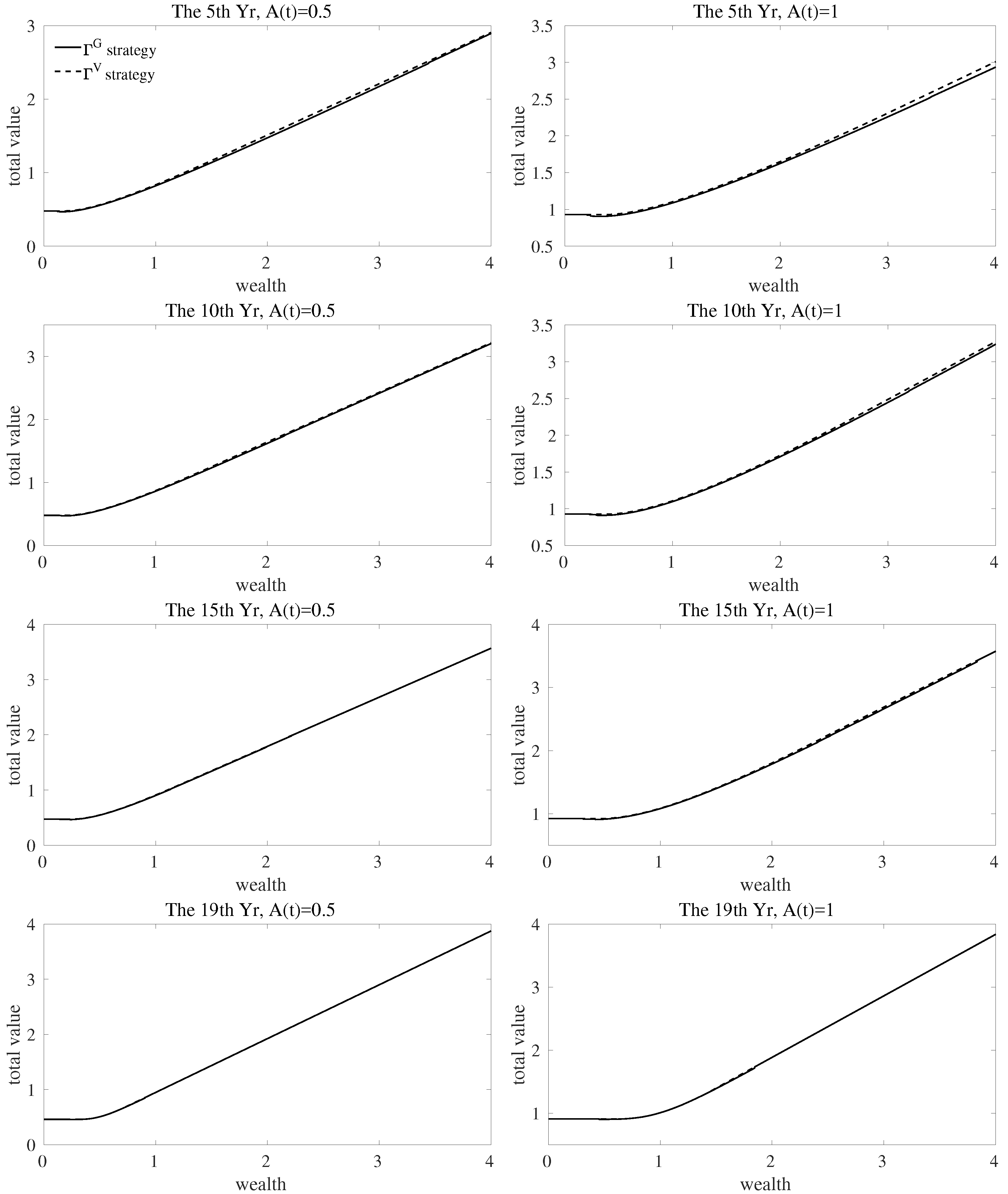
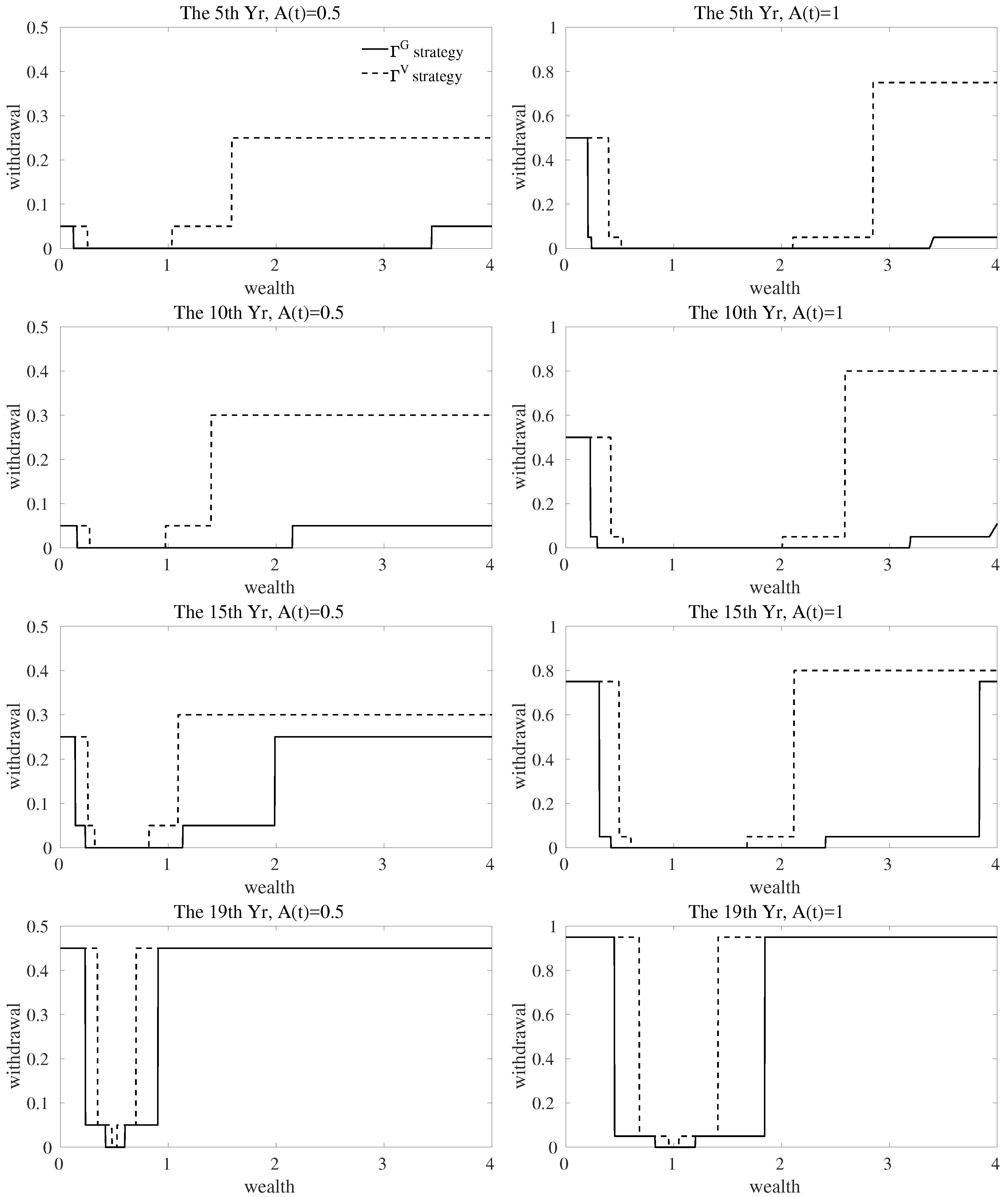
6.1. Withdrawal Strategies When Management Fees Are Present
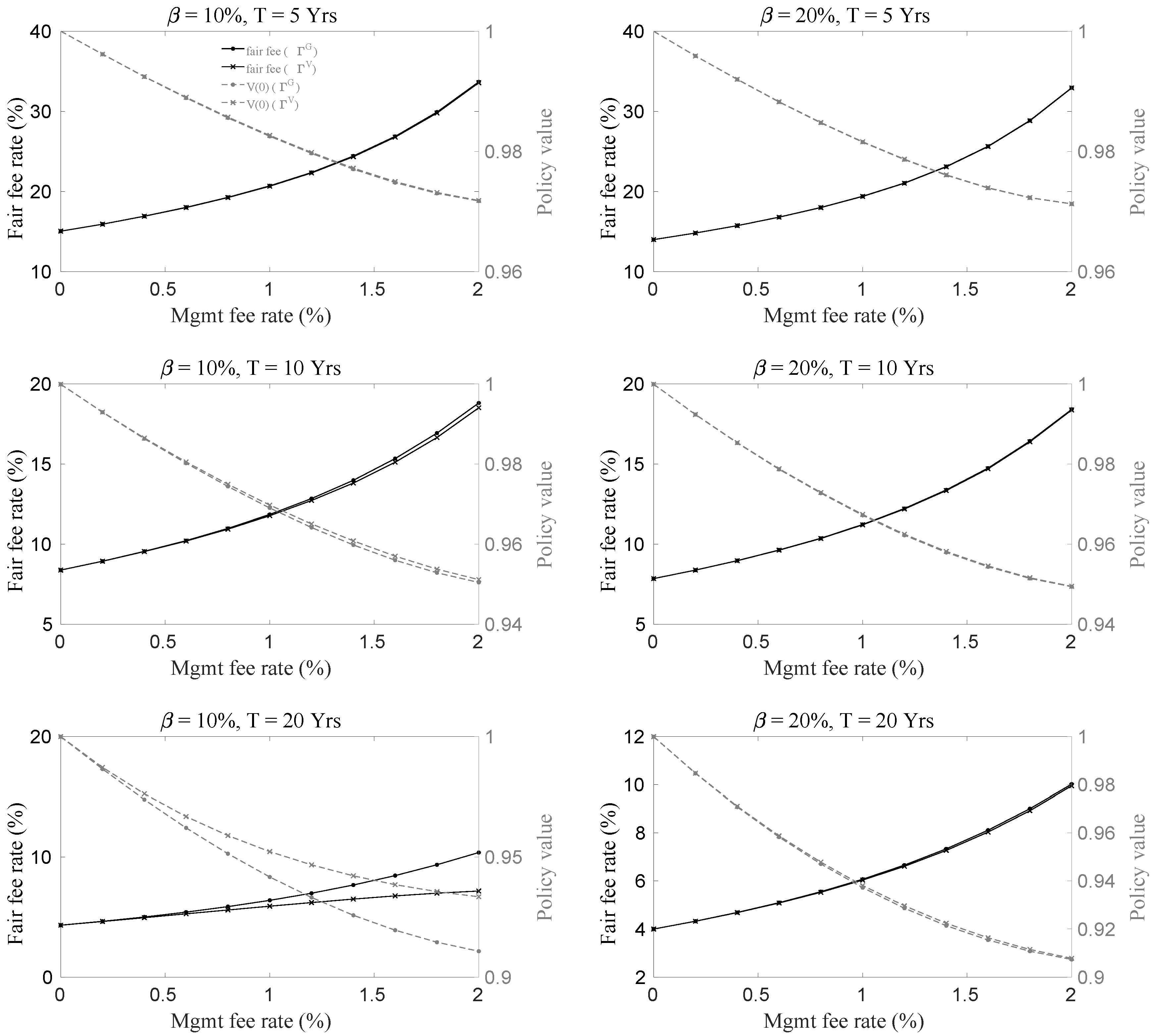
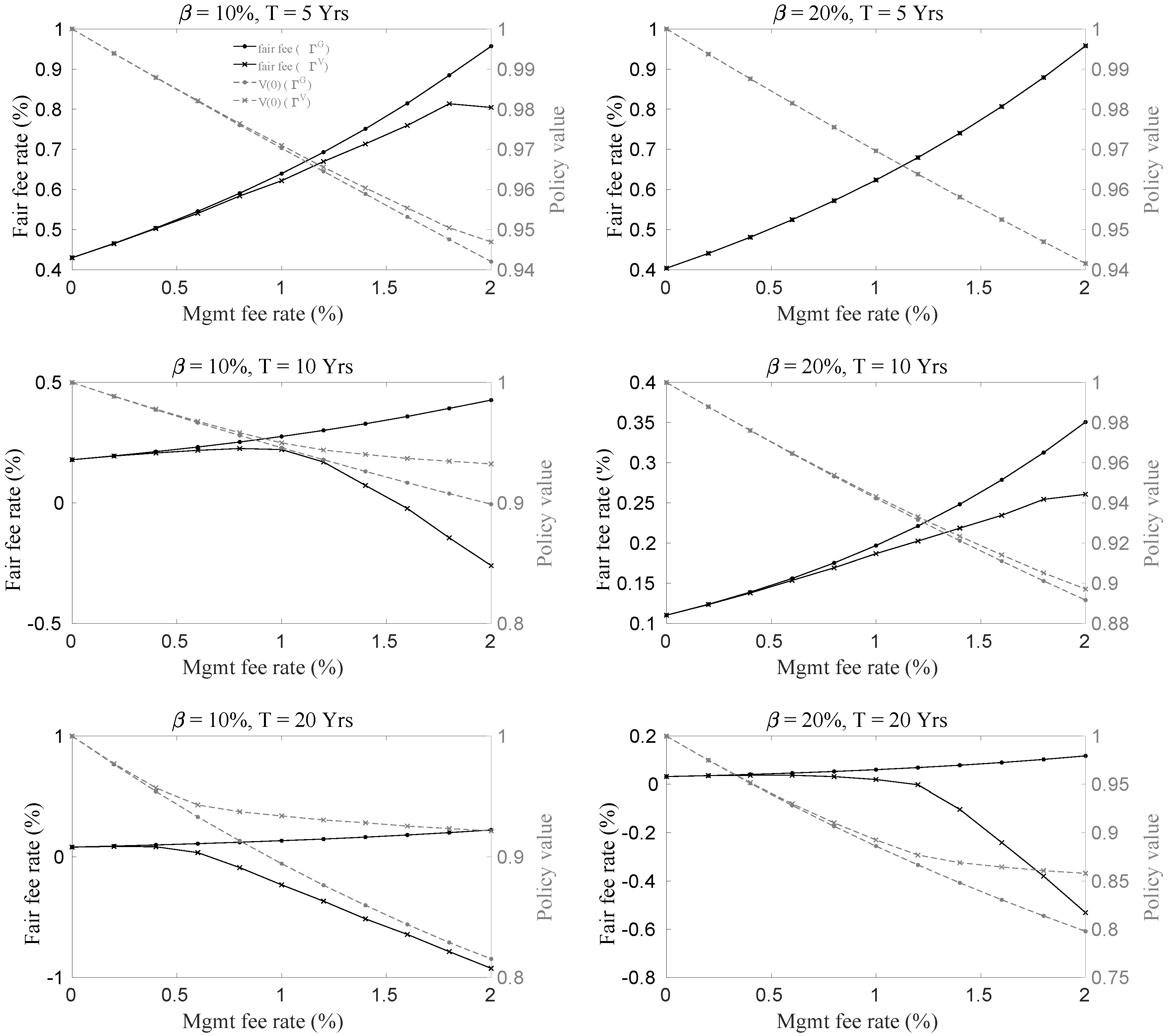
6.2. The Impact of Management Fees on the Fair Insurance Fees
- longer maturity T,
- lower penalty rate ,
- higher interest rate r, and
- higher management fee rate .
7. Conclusions
Author Contributions
Funding
Acknowledgments
Conflicts of Interest
References
- Agapova, Anna. 2011. Conventional mutual index funds versus exchange-traded funds. Journal of Financial Markets 14: 323–43. [Google Scholar] [CrossRef]
- Azimzadeh, Parsiad, and Peter A. Forsyth. 2015. The existence of optimal bang–bang controls for gmxb contracts. SIAM Journal on Financial Mathematics 6: 117–39. [Google Scholar] [CrossRef]
- Bacinello, Anna Rita, and Fulvio Ortu. 1996. Fixed income linked life insurance policies with minimum guarantees: Pricing models and numerical results. European Journal of Operational Research 91: 235–49. [Google Scholar] [CrossRef]
- Bauer, Daniel, Alexander Kling, and Jochen Russ. 2008. A universal pricing framework for guaranteed minimum benefits in variable annuities. ASTIN Bulletin 38: 621–51. [Google Scholar] [CrossRef]
- Bélanger, Amélie C., Peter A. Forsyth, and George Labahn. 2009. Valuing guaranteed minimum death benefit clause with partial withdrawals. Applied Mathematical Finance 16: 451–96. [Google Scholar] [CrossRef]
- Chen, Zhuliang, and Peter A. Forsyth. 2008. A numerical scheme for the impulse control formulation for pricing variable annuities with a guaranteed minimum withdrawal benefit (gmwb). Numerische Mathematik 109: 535–69. [Google Scholar] [CrossRef]
- Chen, Zhang, Ken Vetzal, and Peter A. Forsyth. 2008. The effect of modelling parameters on the value of GMWB guarantees. Insurance: Mathematics and Economics 43: 165–73. [Google Scholar] [CrossRef]
- Cramer, Errol, Patricia Matson, and Larry Rubin. 2007. Common practices relating to fasb statement 133, accounting for derivative instruments and hedging activities as it relates to variable annuities with guaranteed benefits. In Practice Note. Washington, DC: American Academy of Actuaries. [Google Scholar]
- Crank, John, and Phyllis Nicolson. 1947. A practical method for numerical evaluation of solutions of partial differential equations of the heat-conduction type. Mathematical Proceedings of the Cambridge Philosophical Society 43: 50–67. [Google Scholar] [CrossRef]
- Cui, Zhenyu, Runhuan Feng, and Anne MacKay. 2017. Variable annuities with vix-linked fee structure under a heston-type stochastic volatility model. North American Actuarial Journal 21: 458–83. [Google Scholar] [CrossRef]
- Dai, Min, Yue Kuen Kwok, and Jianping Zong. 2008. Guaranteed minimum withdrawal benefit in variable annuities. Mathematical Finance 18: 595–611. [Google Scholar] [CrossRef]
- Delbaen, Freddy, and Walter Schachermayer. 2006. The Mathematics of Arbitrage. Berlin: Springer-Verlag. [Google Scholar]
- Feng, Runhuan, and Huaxiong Huang. 2016. Statutory financial reporting for variable annuity guranteed death benefits: Market practice, mathematical modeling and computation. Insurance: Mathematics and Economics 67: 54–64. [Google Scholar]
- Feng, Runhuan, and Xiaochen Jing. 2016. Analytical valuation and hedging of variable annuity guaranteed lifetime withdrawal benefits. Insurance: Mathematics and Economics 72: 36–48. [Google Scholar] [CrossRef]
- Feng, Runhuan, Xiaochen Jing, and Jan Dhaene. 2017. Comonotonic approximations of risk measures for variable annuity guaranteed benefits with dynamic policyholder behavior. Journal of Computational and Applied Mathematics 311: 272–92. [Google Scholar] [CrossRef]
- Feng, Runhuan, and Jan Vecer. 2017. Risk-based capital requirements for guaranteed minimum withdrawal benefit. Quantitative Finance 17: 471–78. [Google Scholar] [CrossRef]
- Feng, Runhuan, and Hans W. Volkmer. 2012. Analytical calculation of risk measures for variable annuity guaranteed benefits. Insurance: Mathematics and Economics 55: 636–48. [Google Scholar] [CrossRef]
- Feng, Runhuan, and Hans W. Volkmer. 2016. An identity of hitting times and its application to the valuation of guaranteed minimum withdrawal benefit. Mathematics and Financial Economics 10: 127–49. [Google Scholar] [CrossRef]
- Forsyth, Peter, and Kenneth Vetzal. 2014. An optimal stochastic control framework for determining the cost of hedging of variable annuities. Journal of Economic Dynamics and Control 44: 29–53. [Google Scholar] [CrossRef]
- Fung, Man Chung, Katja Ignatieva, and Michael Sherris. 2014. Systematic mortality risk: An analysis of guaranteed lifetime withdrawal benefits in variable annuities. Insurance: Mathematics and Economics 58: 103–15. [Google Scholar]
- Hirsa, Ali. 2012. Computational Methods in Finance. Chapman and Hall/CRC Financial Mathematics Series; Boca Raton: CRC Press. [Google Scholar]
- Ho, Thomas S. Y., Sang Bin Lee, and Yoon Seok Choi. 2005. Practical Considerations in Managing Variable Annuities. Citeseer. Available online: http://citeseerx.ist.psu.edu/viewdoc/download?doi=10.1.1.114.7023&rep=rep1&type=pdf (accessed on 18 September 2018).
- Huang, Yao Tung, and Yue Kuen Kwok. 2016. Regression-based Monte Carlo methods for stochastic control models: Variable annuities with lifelong guarantees. Quantitative Finance 16: 905–28. [Google Scholar] [CrossRef]
- Hyndman, Cody B., and Menachem Wenger. 2014. Valuation perspectives and decompositions for variable annuities. Insurance: Mathematics and Economics 55: 283–90. [Google Scholar]
- Kalberer, Tigran, and Kannoo Ravindran. 2009. Variable Annuities. London: Risk Books. [Google Scholar]
- Kling, Alexander, Frederik Ruez, and Jochen Russ. 2011. The impact of stochastic volatility on pricing, hedging, and hedge efficiency of withdrawal benefit guarantees in variable annuities. ASTIN Bulletin 41: 511–45. [Google Scholar]
- Kostovetsky, Leonard. 2003. Index mutual funds and exchange-traded funds. The Journal of Portfolio Management 29: 80–92. [Google Scholar] [CrossRef]
- Ledlie, M. C., D. P. Corry, G. S. Finkelstein, A. J. Ritchie, Su, and D. C. E. Wilson. 2008. Variable annuities. British Actuarial Journal 14: 327–89. [Google Scholar] [CrossRef]
- Luo, Xiaolin, and Pavel V. Shevchenko. 2015a. Fast numerical method for pricing of variable annuities with guaranteed minimum withdrawal benefit under optimal withdrawal strategy. International Journal of Financial Engineering 2: 1550024:1–26. [Google Scholar] [CrossRef]
- Luo, Xiaolin, and Pavel V. Shevchenko. 2015b. Valuation of variable annuities with guaranteed minimum withdrawal and death benefits via stochastic control optimization. Insurance: Mathematics and Economics 62: 5–15. [Google Scholar]
- Milevsky, Moshe A., and Thomas S. Salisbury. 2006. Financial valuation of guaranteed minimum withdrawal benefits. Insurance: Mathematics and Economics 38: 21–38. [Google Scholar] [CrossRef]
- Moenig, Thorsten, and Daniel Bauer. 2015. Revisiting the risk-neutral approach to optimal policyholder behavior: A study of withdrawal guarantees in variable annuities. Review of Finance 20: 759–94. [Google Scholar] [CrossRef]
- Platen, Eckhard, and David Heath. 2006. A Benchmark Approach to Quantitative Finance. Heidelberg: Springer. [Google Scholar]
- Poterba, James M., and John B. Shoven. 2002. Exchange traded funds: A new investment option for taxable investors. American Economic Review 92: 422–27. [Google Scholar] [CrossRef]
- Shevchenko, Pavel V., and Xiaolin Luo. 2016. A unified pricing of variable annuity guarantees under the optimal stochastic control framework. Risks 4: 22. [Google Scholar] [CrossRef]
- Shevchenko, Pavel V., and Xiaolin Luo. 2017. Valuation of variable annuities with guaranteed minimum withdrawal benefit under stochastic interest rate. Insurance: Mathematics and Economics 76 (SC): 104–17. [Google Scholar] [CrossRef]
- Sun, Peter, Ram Kelkar, Jing Dai, and Victor Huang. 2016. How Effective Is Variable Annuity Guarantee Hedging? Milliman Research Report. Available online: http://au.milliman.com/insight/2016/How-effective-is-variable-annuity-guarantee-hedging (accessed on 18 September 2018).


| Parameters | ||||||||||||||
|---|---|---|---|---|---|---|---|---|---|---|---|---|---|---|
| 1 | 10 | 10 | 5 | 3.08 | 3.48 | 3.96 | 4.59 | 5.41 | 6.65 | 8.66 | 12.18 | 17.67 | 23.53 | 29.92 |
| 10 | 1.66 | 1.92 | 2.25 | 2.66 | 3.21 | 3.97 | 5.08 | 6.77 | 9.26 | 12.17 | 15.31 | |||
| 20 | 0.82 | 0.97 | 1.17 | 1.43 | 1.77 | 2.22 | 2.83 | 3.68 | 4.81 | 6.19 | 7.71 | |||
| 20 | 5 | 3.08 | 3.47 | 3.95 | 4.55 | 5.34 | 6.48 | 8.39 | 12.01 | 17.66 | 23.55 | 29.92 | ||
| 10 | 1.66 | 1.91 | 2.23 | 2.62 | 3.13 | 3.83 | 4.88 | 6.60 | 9.20 | 12.17 | 15.31 | |||
| 20 | 0.81 | 0.96 | 1.16 | 1.40 | 1.71 | 2.13 | 2.72 | 3.57 | 4.74 | 6.17 | 7.71 | |||
| 30 | 10 | 5 | 15.05 | 15.92 | 16.92 | 18.02 | 19.27 | 20.70 | 22.37 | 24.43 | 26.88 | 29.91 | 33.69 | |
| 10 | 8.38 | 8.93 | 9.55 | 10.22 | 10.98 | 11.85 | 12.84 | 13.98 | 15.34 | 16.93 | 18.81 | |||
| 20 | 4.32 | 4.64 | 5.00 | 5.41 | 5.87 | 6.39 | 6.98 | 7.66 | 8.45 | 9.35 | 10.37 | |||
| 20 | 5 | 13.99 | 14.82 | 15.73 | 16.80 | 18.01 | 19.40 | 21.06 | 23.11 | 25.64 | 28.86 | 32.95 | ||
| 10 | 7.85 | 8.38 | 8.97 | 9.63 | 10.36 | 11.22 | 12.22 | 13.38 | 14.74 | 16.43 | 18.41 | |||
| 20 | 4.00 | 4.33 | 4.69 | 5.10 | 5.55 | 6.07 | 6.66 | 7.34 | 8.11 | 9.01 | 10.02 | |||
| 5 | 10 | 10 | 5 | 0.43 | 0.47 | 0.50 | 0.55 | 0.59 | 0.64 | 0.69 | 0.75 | 0.81 | 0.88 | 0.96 |
| 10 | 0.18 | 0.20 | 0.21 | 0.23 | 0.25 | 0.28 | 0.30 | 0.33 | 0.36 | 0.39 | 0.43 | |||
| 20 | 0.08 | 0.09 | 0.10 | 0.11 | 0.12 | 0.13 | 0.15 | 0.16 | 0.18 | 0.20 | 0.22 | |||
| 20 | 5 | 0.40 | 0.44 | 0.48 | 0.52 | 0.57 | 0.62 | 0.68 | 0.74 | 0.81 | 0.88 | 0.96 | ||
| 10 | 0.11 | 0.12 | 0.14 | 0.16 | 0.18 | 0.20 | 0.22 | 0.25 | 0.28 | 0.31 | 0.35 | |||
| 20 | 0.03 | 0.04 | 0.04 | 0.05 | 0.05 | 0.06 | 0.07 | 0.08 | 0.09 | 0.10 | 0.12 | |||
| 30 | 10 | 5 | 5.33 | 5.48 | 5.65 | 5.81 | 5.99 | 6.17 | 6.35 | 6.55 | 6.75 | 6.96 | 7.17 | |
| 10 | 2.91 | 3.02 | 3.12 | 3.23 | 3.35 | 3.47 | 3.60 | 3.73 | 3.86 | 4.01 | 4.16 | |||
| 20 | 1.58 | 1.65 | 1.74 | 1.82 | 1.91 | 2.00 | 2.10 | 2.21 | 2.32 | 2.43 | 2.55 | |||
| 20 | 5 | 4.97 | 5.13 | 5.28 | 5.44 | 5.61 | 5.79 | 5.97 | 6.15 | 6.35 | 6.55 | 6.76 | ||
| 10 | 2.27 | 2.35 | 2.43 | 2.52 | 2.61 | 2.71 | 2.81 | 2.91 | 3.02 | 3.13 | 3.25 | |||
| 20 | 1.08 | 1.13 | 1.19 | 1.24 | 1.31 | 1.37 | 1.43 | 1.50 | 1.58 | 1.65 | 1.73 | |||
| Parameters | ||||||||||||||
|---|---|---|---|---|---|---|---|---|---|---|---|---|---|---|
| 1 | 10 | 10 | 5 | 3.08 | 3.47 | 3.96 | 4.57 | 5.36 | 6.57 | 8.55 | 12.12 | 17.66 | 23.55 | 29.93 |
| 10 | 1.66 | 1.92 | 2.23 | 2.61 | 3.13 | 3.81 | 4.86 | 6.44 | 8.99 | 12.11 | 15.30 | |||
| 20 | 0.82 | 0.96 | 1.09 | 1.21 | 1.33 | 1.44 | 1.50 | 1.59 | 1.65 | 1.70 | 1.81 | |||
| 20 | 5 | 3.08 | 3.47 | 3.95 | 4.55 | 5.34 | 6.48 | 8.38 | 12.01 | 17.66 | 23.55 | 29.92 | ||
| 10 | 1.66 | 1.91 | 2.23 | 2.62 | 3.12 | 3.80 | 4.84 | 6.56 | 9.19 | 12.17 | 15.31 | |||
| 20 | 0.81 | 0.96 | 1.16 | 1.39 | 1.67 | 2.05 | 2.60 | 3.43 | 4.65 | 6.14 | 7.70 | |||
| 30 | 10 | 5 | 15.05 | 15.92 | 16.91 | 18.00 | 19.25 | 20.66 | 22.32 | 24.34 | 26.79 | 29.80 | 33.58 | |
| 10 | 8.38 | 8.93 | 9.53 | 10.19 | 10.93 | 11.77 | 12.72 | 13.81 | 15.11 | 16.65 | 18.51 | |||
| 20 | 4.32 | 4.63 | 4.94 | 5.27 | 5.59 | 5.90 | 6.20 | 6.49 | 6.76 | 6.99 | 7.16 | |||
| 20 | 5 | 13.99 | 14.82 | 15.73 | 16.80 | 18.00 | 19.39 | 21.04 | 23.09 | 25.62 | 28.84 | 32.93 | ||
| 10 | 7.85 | 8.38 | 8.96 | 9.62 | 10.35 | 11.20 | 12.19 | 13.34 | 14.70 | 16.38 | 18.37 | |||
| 20 | 4.00 | 4.32 | 4.68 | 5.08 | 5.53 | 6.04 | 6.61 | 7.27 | 8.04 | 8.92 | 9.95 | |||
| 5 | 10 | 10 | 5 | 0.43 | 0.47 | 0.50 | 0.54 | 0.58 | 0.62 | 0.67 | 0.71 | 0.76 | 0.81 | 0.80 |
| 10 | 0.18 | 0.19 | 0.21 | 0.22 | 0.23 | 0.22 | 0.17 | 0.07 | −0.02 | −0.14 | −0.26 | |||
| 20 | 0.08 | 0.09 | 0.08 | 0.04 | −0.09 | −0.23 | −0.37 | −0.51 | −0.64 | −0.79 | −0.93 | |||
| 20 | 5 | 0.40 | 0.44 | 0.48 | 0.52 | 0.57 | 0.62 | 0.68 | 0.74 | 0.81 | 0.88 | 0.96 | ||
| 10 | 0.11 | 0.12 | 0.14 | 0.15 | 0.17 | 0.19 | 0.20 | 0.22 | 0.23 | 0.25 | 0.26 | |||
| 20 | 0.03 | 0.04 | 0.04 | 0.04 | 0.03 | 0.02 | −0.00 | −0.10 | −0.24 | −0.38 | −0.53 | |||
| 30 | 10 | 5 | 5.33 | 5.48 | 5.64 | 5.79 | 5.95 | 6.11 | 6.27 | 6.43 | 6.60 | 6.75 | 6.94 | |
| 10 | 2.91 | 3.01 | 3.10 | 3.18 | 3.26 | 3.34 | 3.41 | 3.47 | 3.53 | 3.58 | 3.60 | |||
| 20 | 1.58 | 1.64 | 1.68 | 1.72 | 1.74 | 1.75 | 1.75 | 1.74 | 1.74 | 1.73 | 1.71 | |||
| 20 | 5 | 4.97 | 5.13 | 5.28 | 5.44 | 5.61 | 5.78 | 5.96 | 6.14 | 6.32 | 6.51 | 6.70 | ||
| 10 | 2.27 | 2.35 | 2.43 | 2.51 | 2.59 | 2.67 | 2.74 | 2.82 | 2.88 | 2.94 | 3.00 | |||
| 20 | 1.08 | 1.13 | 1.18 | 1.22 | 1.23 | 1.24 | 1.23 | 1.21 | 1.18 | 1.14 | 1.09 | |||
| Parameters | ||||||||||||||
|---|---|---|---|---|---|---|---|---|---|---|---|---|---|---|
| 1 | 10 | 10 | 5 | 1.00 | 0.99 | 0.99 | 0.98 | 0.98 | 0.98 | 0.97 | 0.97 | 0.97 | 0.97 | 0.97 |
| 10 | 1.00 | 0.99 | 0.98 | 0.97 | 0.97 | 0.96 | 0.95 | 0.95 | 0.95 | 0.95 | 0.95 | |||
| 20 | 1.00 | 0.98 | 0.96 | 0.95 | 0.94 | 0.92 | 0.92 | 0.91 | 0.90 | 0.90 | 0.90 | |||
| 20 | 5 | 1.00 | 0.99 | 0.99 | 0.98 | 0.98 | 0.98 | 0.97 | 0.97 | 0.97 | 0.97 | 0.97 | ||
| 10 | 1.00 | 0.99 | 0.98 | 0.97 | 0.96 | 0.96 | 0.95 | 0.95 | 0.95 | 0.95 | 0.95 | |||
| 20 | 1.00 | 0.98 | 0.96 | 0.95 | 0.93 | 0.92 | 0.91 | 0.91 | 0.90 | 0.90 | 0.90 | |||
| 30 | 10 | 5 | 1.00 | 1.00 | 0.99 | 0.99 | 0.99 | 0.98 | 0.98 | 0.98 | 0.97 | 0.97 | 0.97 | |
| 10 | 1.00 | 0.99 | 0.99 | 0.98 | 0.97 | 0.97 | 0.96 | 0.96 | 0.96 | 0.95 | 0.95 | |||
| 20 | 1.00 | 0.99 | 0.97 | 0.96 | 0.95 | 0.94 | 0.93 | 0.93 | 0.92 | 0.91 | 0.91 | |||
| 20 | 5 | 1.00 | 1.00 | 0.99 | 0.99 | 0.98 | 0.98 | 0.98 | 0.98 | 0.97 | 0.97 | 0.97 | ||
| 10 | 1.00 | 0.99 | 0.99 | 0.98 | 0.97 | 0.97 | 0.96 | 0.96 | 0.95 | 0.95 | 0.95 | |||
| 20 | 1.00 | 0.98 | 0.97 | 0.96 | 0.95 | 0.94 | 0.93 | 0.92 | 0.92 | 0.91 | 0.91 | |||
| 5 | 10 | 10 | 5 | 1.00 | 0.99 | 0.99 | 0.98 | 0.98 | 0.97 | 0.96 | 0.96 | 0.95 | 0.95 | 0.94 |
| 10 | 1.00 | 0.99 | 0.98 | 0.97 | 0.96 | 0.95 | 0.94 | 0.93 | 0.92 | 0.91 | 0.90 | |||
| 20 | 1.00 | 0.98 | 0.95 | 0.93 | 0.91 | 0.89 | 0.88 | 0.86 | 0.84 | 0.83 | 0.82 | |||
| 20 | 5 | 1.00 | 0.99 | 0.99 | 0.98 | 0.98 | 0.97 | 0.96 | 0.96 | 0.95 | 0.95 | 0.94 | ||
| 10 | 1.00 | 0.99 | 0.98 | 0.96 | 0.95 | 0.94 | 0.93 | 0.92 | 0.91 | 0.90 | 0.89 | |||
| 20 | 1.00 | 0.97 | 0.95 | 0.93 | 0.91 | 0.89 | 0.87 | 0.85 | 0.83 | 0.81 | 0.80 | |||
| 30 | 10 | 5 | 1.00 | 1.00 | 0.99 | 0.99 | 0.98 | 0.98 | 0.97 | 0.97 | 0.96 | 0.96 | 0.96 | |
| 10 | 1.00 | 0.99 | 0.98 | 0.98 | 0.97 | 0.96 | 0.95 | 0.95 | 0.94 | 0.93 | 0.93 | |||
| 20 | 1.00 | 0.98 | 0.97 | 0.96 | 0.94 | 0.93 | 0.92 | 0.91 | 0.90 | 0.89 | 0.88 | |||
| 20 | 5 | 1.00 | 0.99 | 0.99 | 0.98 | 0.98 | 0.97 | 0.97 | 0.96 | 0.96 | 0.95 | 0.95 | ||
| 10 | 1.00 | 0.99 | 0.98 | 0.97 | 0.96 | 0.95 | 0.94 | 0.93 | 0.92 | 0.91 | 0.91 | |||
| 20 | 1.00 | 0.98 | 0.96 | 0.94 | 0.92 | 0.90 | 0.89 | 0.87 | 0.86 | 0.84 | 0.83 | |||
| Parameters | ||||||||||||||
|---|---|---|---|---|---|---|---|---|---|---|---|---|---|---|
| 1 | 10 | 10 | 5 | 1.00 | 0.99 | 0.99 | 0.98 | 0.98 | 0.98 | 0.97 | 0.97 | 0.97 | 0.97 | 0.97 |
| 10 | 1.00 | 0.99 | 0.98 | 0.97 | 0.97 | 0.96 | 0.95 | 0.95 | 0.95 | 0.95 | 0.95 | |||
| 20 | 1.00 | 0.98 | 0.97 | 0.96 | 0.95 | 0.95 | 0.94 | 0.94 | 0.94 | 0.93 | 0.93 | |||
| 20 | 5 | 1.00 | 0.99 | 0.99 | 0.98 | 0.98 | 0.98 | 0.97 | 0.97 | 0.97 | 0.97 | 0.97 | ||
| 10 | 1.00 | 0.99 | 0.98 | 0.97 | 0.96 | 0.96 | 0.95 | 0.95 | 0.95 | 0.95 | 0.95 | |||
| 20 | 1.00 | 0.98 | 0.96 | 0.95 | 0.93 | 0.92 | 0.91 | 0.91 | 0.90 | 0.90 | 0.90 | |||
| 30 | 10 | 5 | 1.00 | 1.00 | 0.99 | 0.99 | 0.99 | 0.98 | 0.98 | 0.98 | 0.97 | 0.97 | 0.97 | |
| 10 | 1.00 | 0.99 | 0.99 | 0.98 | 0.97 | 0.97 | 0.97 | 0.96 | 0.96 | 0.95 | 0.95 | |||
| 20 | 1.00 | 0.99 | 0.98 | 0.97 | 0.96 | 0.95 | 0.95 | 0.94 | 0.94 | 0.94 | 0.93 | |||
| 20 | 5 | 1.00 | 1.00 | 0.99 | 0.99 | 0.98 | 0.98 | 0.98 | 0.98 | 0.97 | 0.97 | 0.97 | ||
| 10 | 1.00 | 0.99 | 0.99 | 0.98 | 0.97 | 0.97 | 0.96 | 0.96 | 0.95 | 0.95 | 0.95 | |||
| 20 | 1.00 | 0.98 | 0.97 | 0.96 | 0.95 | 0.94 | 0.93 | 0.92 | 0.92 | 0.91 | 0.91 | |||
| 5 | 10 | 10 | 5 | 1.00 | 0.99 | 0.99 | 0.98 | 0.98 | 0.97 | 0.97 | 0.96 | 0.96 | 0.95 | 0.95 |
| 10 | 1.00 | 0.99 | 0.98 | 0.97 | 0.96 | 0.95 | 0.94 | 0.94 | 0.94 | 0.93 | 0.93 | |||
| 20 | 1.00 | 0.98 | 0.96 | 0.94 | 0.94 | 0.93 | 0.93 | 0.93 | 0.93 | 0.92 | 0.92 | |||
| 20 | 5 | 1.00 | 0.99 | 0.99 | 0.98 | 0.98 | 0.97 | 0.96 | 0.96 | 0.95 | 0.95 | 0.94 | ||
| 10 | 1.00 | 0.99 | 0.98 | 0.96 | 0.95 | 0.94 | 0.93 | 0.92 | 0.91 | 0.91 | 0.90 | |||
| 20 | 1.00 | 0.97 | 0.95 | 0.93 | 0.91 | 0.89 | 0.88 | 0.87 | 0.86 | 0.86 | 0.86 | |||
| 30 | 10 | 5 | 1.00 | 1.00 | 0.99 | 0.99 | 0.98 | 0.98 | 0.97 | 0.97 | 0.97 | 0.96 | 0.96 | |
| 10 | 1.00 | 0.99 | 0.98 | 0.98 | 0.97 | 0.97 | 0.96 | 0.96 | 0.95 | 0.95 | 0.95 | |||
| 20 | 1.00 | 0.99 | 0.97 | 0.97 | 0.96 | 0.95 | 0.94 | 0.94 | 0.94 | 0.93 | 0.93 | |||
| 20 | 5 | 1.00 | 0.99 | 0.99 | 0.98 | 0.98 | 0.97 | 0.97 | 0.96 | 0.96 | 0.95 | 0.95 | ||
| 10 | 1.00 | 0.99 | 0.98 | 0.97 | 0.96 | 0.95 | 0.94 | 0.94 | 0.93 | 0.92 | 0.92 | |||
| 20 | 1.00 | 0.98 | 0.96 | 0.94 | 0.93 | 0.92 | 0.91 | 0.90 | 0.89 | 0.88 | 0.88 | |||
© 2018 by the authors. Licensee MDPI, Basel, Switzerland. This article is an open access article distributed under the terms and conditions of the Creative Commons Attribution (CC BY) license (http://creativecommons.org/licenses/by/4.0/).
Share and Cite
Sun, J.; Shevchenko, P.V.; Fung, M.C. The Impact of Management Fees on the Pricing of Variable Annuity Guarantees. Risks 2018, 6, 103. https://doi.org/10.3390/risks6030103
Sun J, Shevchenko PV, Fung MC. The Impact of Management Fees on the Pricing of Variable Annuity Guarantees. Risks. 2018; 6(3):103. https://doi.org/10.3390/risks6030103
Chicago/Turabian StyleSun, Jin, Pavel V. Shevchenko, and Man Chung Fung. 2018. "The Impact of Management Fees on the Pricing of Variable Annuity Guarantees" Risks 6, no. 3: 103. https://doi.org/10.3390/risks6030103
APA StyleSun, J., Shevchenko, P. V., & Fung, M. C. (2018). The Impact of Management Fees on the Pricing of Variable Annuity Guarantees. Risks, 6(3), 103. https://doi.org/10.3390/risks6030103