Grouped Normal Variance Mixtures

Abstract

Grouped normal variance mixtures are a class of multivariate distributions that generalize classical normal variance mixtures such as the multivariate t distribution, by allowing different groups to have different (comonotone) mixing distributions. This allows one to better model risk factors where components within a group are of similar type, but where different groups have components of quite different type. This paper provides an encompassing body of algorithms to address the computational challenges when working with this class of distributions. In particular, the distribution function and copula are estimated efficiently using randomized quasi-Monte Carlo (RQMC) algorithms. We propose to estimate the log-density function, which is in general not available in closed form, using an adaptive RQMC scheme. This, in turn, gives rise to a likelihood-based fitting procedure to jointly estimate the parameters of a grouped normal mixture copula jointly. We also provide mathematical expressions and methods to compute Kendall’s tau, Spearman’s rho and the tail dependence coefficient $\lambda$. All algorithms presented are available in the R package nvmix (version ≥ 0.0.5).

1. Introduction

It is well known that for the purpose of modeling dependence in a risk management setting, the multivariate normal distribution is not flexible enough, and therefore its use can lead to a misleading assessment of risk(s). Indeed, the multivariate normal has light tails and its copula is tail-independent such that inference based on this model heavily underestimates joint extreme events. An important class of distributions that generalizes this simple model is that of normal variance mixtures. A random vector $\mathit{X}=(X_1,\dots ,X_d)$ follows a normal variance mixture, denoted by $\mathit{X}\sim {\mathrm{NVM}}_d(\mathit{\mu },\mathsf{\Sigma },F_W)$, if, in distribution,

$$\begin{array}{c}\hfill \mathit{X}=\mathit{\mu }+\sqrt{W}A\mathit{Z},\end{array}$$

(1)

where $\mathit{\mu }\in {\mathbb{R}}^d$ is the location (vector), $\mathsf{\Sigma }=A{A}^{\top }$ for $A\in {\mathbb{R}}^{d\times k}$ denotes the symmetric, positive semidefinite scale (matrix) and $W\sim F_W$ is a non-negative random variable independent of the random vector $\mathit{Z}\sim N_k(\mathbf{0},I_k)$ (where $I_k\in {\mathbb{R}}^{k\times k}$ denotes the identity matrix); see, for example, (McNeil et al. 2015, Section 6.2) or (Hintz et al. 2020). Here, the random variable W can be thought of as a shock mixing the normal $\mathit{Z}$, thus allowing $\mathit{X}$ to have different tail behavior and dependence structure than the special case of a multivariate normal.

The multivariate t distribution with $\nu >0$ degrees of freedom (dof) is also a special case of (1), for $W\sim IG(\nu /2,\nu /2)$; a random variable (rv) W is said to follow an inverse-gamma distribution with shape $\alpha >0$ and rate $\beta >0$, notation $W\sim IG(\alpha ,\beta )$, if W has density $f_W\left(w\right)={\beta }^{-\alpha }{w}^{-\alpha -1}exp(-1/\left(\beta w\right))/\mathsf{\Gamma }\left(\alpha \right)$ for $w>0$ (here, $\mathsf{\Gamma }\left(x\right)={\int }_0^{\infty }{t}^{x-1}exp(-t)\mathrm{d}t$ denotes the gamma function). If $W\sim IG(\nu /2,\nu /2)$, then $X_j\sim t_{\nu }({\mu }_j,{\mathsf{\Sigma }}_{jj})$, $j=1,\dots ,d$, so that all margins are univariate t with the same dof $\nu$. The t copula, which is the implicitly derived copula from $\mathit{X}\sim t_d(\nu ,\mathbf{0},P)$ for a correlation matrix P via Sklar’s theorem, is a widely used copula in risk management; see, e.g., Demarta and McNeil (2005). It allows one to model pairwise dependencies, including tail dependence, flexibly via the correlation matrix P. When $P=I_d$, all k-dimensional margins of $\mathit{X}$ are identically distributed. To overcome this limitation, one can allow different margins to have different dof. On a copula level, this leads to the notion of grouped t copulas of Daul et al. (2003) and generalized t copulas of Luo and Shevchenko (2010).

In this paper, we, more generally, define grouped normal variance mixtures via the stochastic representation

$$\begin{array}{c}\hfill \mathit{X}=\mathit{\mu }+Diag\left(\sqrt{\mathit{W}}\right)A\mathit{Z},\end{array}$$

(2)

where $\mathit{W}=(W_1,\dots ,W_d)$ is a d-dimensional non-negative and comonotone random vector with $W_j\sim F_{W_j}$ that is independent of $\mathit{Z}$. Denote by $F_W^{\leftarrow }\left(u\right)=inf\{w\ge 0:F_W\left(w\right)\ge u\}$ the quantile function of a random variable W. Comonotonicity of the $W_j$ implies the stochastic representation

$$\begin{array}{c}\hfill \mathit{W}=(W_1,\dots ,W_d)=(F_{W_1}^{\leftarrow }\left(U\right),\dots ,F_{W_d}^{\leftarrow }\left(U\right)),U\sim \mathrm{U}(0,1).\end{array}$$

(3)

If a d-dimensional random vector $\mathit{X}$ satisfies (2) with $\mathit{W}$ given as in (3), we use the notation $\mathit{X}\sim \mathrm{gNVM}(\mathit{\mu },\mathsf{\Sigma },F_{\mathit{W}})$ where $F_{\mathit{W}}\left(\mathit{w}\right)=\mathbb{P}(\mathit{W}\le \mathit{w})$ for $\mathit{w}\in {\mathbb{R}}^d$ and the inequality is understood component-wise.

As mentioned above, in the case of an (ungrouped) normal variance mixture distribution from (1), the scalar random variable (rv) W can be regarded as a shock affecting all components of $\mathit{X}$. In the more general setting considered in this paper where $\mathit{W}$ is a vector of comonotone mixing rvs, different, perfectly dependent random variables affect different margins of $\mathit{X}$. By moving from a scalar mixing rv to a comonotone random vector, one obtains non-elliptical distributions well beyond the classical multivariate t case, giving rise to flexible modeling of joint and marginal body and tail behaviors. The price to pay for this generalization is significant computational challenges: Not even the density of a grouped t distribution is available in closed form.

At first glance, the definition given in (2) does not indicate any “grouping” yet. However, Equation (3) allows one to group components of the random vector $\mathit{X}$ such that all components within a group have the same mixing distribution. More precisely, let $\mathit{W}$ be split into S sub-vectors, i.e., $\mathit{W}=({\mathit{W}}_1,\dots ,{\mathit{W}}_S)$ where ${\mathit{W}}_k$ has dimension $d_k$ for $k=1,\dots ,S$ and ${\sum }_{k=1}^S{d}_k=d$. Now let each ${\mathit{W}}_k$ have stochastic representation ${\mathit{W}}_k=(F_{W_k}^{\leftarrow }\left(U\right),\dots ,F_{W_k}^{\leftarrow }\left(U\right))$. Hence, all univariate margins of the subvector ${\mathit{W}}_k$ are identically distributed. This implies that all margins of the corresponding subvector ${\mathit{X}}_k$ are of the same type.

An example is the copula derived from $\mathit{X}$ in (2) when $F_{W_k}=IG\left({\nu }_k/2,{\nu }_k/2\right)$ for $k=1,\dots ,S$; this is the aforementioned grouped t copula. Here, different margins of the copula follow (potentially) different t copulas with different dof, allowing for more flexibility in modeling pairwise dependencies. A grouped t copula with $S=d$, that is when each component has their own mixing distribution, was proposed in Venter et al. (2007) (therein called “individuated t copula”) and studied in more detail in  Luo and Shevchenko (2010) (therein called “t copula with multiple dof”). If $S=1$, the classical t copula with exactly one dof parameter is recovered.

For notational convenience, derivations in this paper are often done for the case $S=d$, so that the $F_{W_j}$ are all different; the case $S<d$, that is when grouping is present, is merely a special case where some of the $F_{W_j}$ are identical. That being said, we chose to keep the name “grouped” to refer to this class of models so as to reflect the original motivation for this type of model, e.g., as in Daul et al. (2003), where it is used to model the components of a portfolio in which there are subgroups representing different business sectors.

Previous work on grouped t copulas and their corresponding distributions includes some algorithms for the tasks needed to handle these models, but were mostly focused on demonstrating the superiority of this class of models over special cases such as the multivariate normal or t distribution. More precisely, in Daul et al. (2003), the grouped t copula was introduced and applied to model an internationally diversified credit portfolio of 92 risk factors split into 8 subgroups. It was demonstrated that the grouped t copula is superior to both the Gaussian and t copula in regards to modeling the tail dependence present in the data. Luo and Shevchenko (2010) also study the grouped t copula and, unlike in Daul et al. (2003), allow group sizes of 1 (corresponding to $S=d$ in our definition). They provide calibration methods to fit the copula to data and furthermore study bivariate characteristics of the grouped t copula, including symmetry properties and tail dependence.

However, to the best of our knowledge, there currently does not exist an encompassing body of work providing all algorithms and formulas required to handle these copulas and their corresponding distributions, both in terms of evaluating distributional quantities and in terms of general fitting algorithms. In particular, not even the problem of computing the distribution and density function of a grouped t copula has been addressed. Our paper fills this gap by providing a complete set of algorithms for performing the main computational tasks associated with these distributions and their associated copulas, and does so in an as automated way as possible. This is done not only for grouped t copulas, but (in many cases) for the more general grouped normal variance mixture distributions/copulas, which allow for even further flexibility in modeling the shock variables $\mathit{W}$. Furthermore, we assume that the only available information about the distribution of the $W_j$ are the marginal quantile functions in the form of a “black box“, meaning that we can only evaluate these quantile functions but have no mathematical expression for them (so that neither the density, nor the distribution function of $W_j$ are available in closed form).

Our work includes the following contributions: (i) we develop an algorithm to evaluate the distribution function of a grouped NVM model. Our method only requires the user to provide a function that evaluates the quantile function of the $W_j$ through a black box. As such, different mixing distributions can be studied by merely providing a quantile function without having to implement an integration routine for the model at hand; (ii) as mentioned above, the density function for a grouped t distribution does not exist in closed form, neither does it for the more general grouped NVM case. We provide an adaptive algorithm to estimate this density function in a very general setting. The adaptive mechanism we propose ensures the estimation procedure is precise even for points that are far from the mean; (iii) to estimate Kendall’s tau and Spearman’s rho for a two-dimensional grouped NVM copula, we provide a representation as an expectation, which in turn leads to an easy-to-approximate two- or three-dimensional integral; (iv) we provide an algorithm to estimate the copula and its density associated with the grouped t copula, and fitting algorithms to estimate the parameters of a grouped NVM copula based on a dataset. While the problem of parameter estimation was already studied in Daul et al. (2003) and Luo and Shevchenko (2010), the computation of the copula density which is required for the joint estimation of all dof parameters has not been investigated in full generality for arbitrary dimensions yet, which is a gap we fill in this paper.

The four items from the list of contributions described in the previous paragraph correspond to Section 3, Section 4, Section 5 and Section 6 of the paper. Section 2 includes a brief presentation of the notation used, basic properties of grouped NVM distributions and a description of randomized quasi-Monte Carlo methods that are used throughout the paper since most quantities of interest require the approximation of integrals. Section 7 provides a discussion. The proofs are given in Section 8.

All our methods are implemented in the R package nvmix (Hofert et al. (2020)) and all numerical results are reproducible with the demo grouped_mixtures.

2. Notation, Basic Properties and Tools

This section provides the necessary background, notations and tools needed throughout the remainder of this paper. The first part addresses some properties of grouped normal variance mixtures, such as mean, covariance and the relationship with elliptical distributions. The second part of this section describes randomized quasi-Monte Carlo methods, which is the type of integration method we apply to approximate quantities that are expressed as expectations, such as the distribution function of grouped normal variance mixtures.

2.1. Grouped Normal Variance Mixtures

To simplify the notation throughout the remainder of this paper, we use the shorthand notations $F_{\mathit{W}}^{\leftarrow }\left(U\right)=(F_{W_1}^{\leftarrow }\left(U\right),\dots ,F_{W_d}^{\leftarrow }\left(U\right))$, ${\mathit{W}}^{\mathrm{D}}=Diag\left(\mathit{W}\right)$, ${\mathit{W}}^{\mathrm{D}}\left(U\right)=Diag\left(F_{\mathit{W}}^{\leftarrow }\left(U\right)\right)$; ${\sqrt{\mathit{W}}}^{\mathrm{D}}$, ${(1/\mathit{W})}^{\mathrm{D}}$ as well as ${(1/\sqrt{\mathit{W}})}^{\mathrm{D}}$ are defined similarly.

Many properties of grouped normal variance mixtures are derived by conditioning on the d-dimensional random vector $\mathit{W}$, or equivalently by conditioning on the underlying univariate uniform rv U. Indeed,

$$\begin{array}{c}\hfill \mathit{X}\mid \mathit{W}\sim N_d\left(\mathit{\mu },{\sqrt{\mathit{W}}}^{\mathrm{D}}\mathsf{\Sigma }{\sqrt{\mathit{W}}}^{\mathrm{D}}\right)\mathrm{or}\mathrm{equivalently}\mathit{X}\mid U\sim N_d\left(\mathit{\mu },{\sqrt{\mathit{W}}}^{\mathrm{D}}\left(U\right)\mathsf{\Sigma }{\sqrt{\mathit{W}}}^{\mathrm{D}}\left(U\right)\right),\end{array}$$

where $N_d(\mathit{\mu },\mathsf{\Sigma })$ denotes the d-dimensional multivariate normal distribution with mean vector $\mathit{\mu }$ and covariance matrix $\mathsf{\Sigma }$. One can see that $\mathit{W}$ “mixes“ the covariance matrix of a multivariate normal and can be regarded as a shock affecting all components of $\mathit{X}$.

2.1.1. Mean and Covariance

If $\mathbb{E}\left(\sqrt{\mathit{W}}\right)$ exists, then $\mathbb{E}\left(\mathit{X}\right)=\mathit{\mu }$, and if $\mathbb{E}\left(\mathit{W}\right)<\infty$, then $cov\left(\mathit{X}\right)=\mathbb{E}\left({\sqrt{\mathit{W}}}^{\mathrm{D}}\mathsf{\Sigma }{\sqrt{\mathit{W}}}^{\mathrm{D}}\right)$. Furthermore, $corr\left(\mathit{X}\right)=P$, where P denotes the correlation matrix corresponding to $\mathsf{\Sigma }$. If $A=I_d$, the (uncorrelated) components of $\mathit{X}$ are independent if and only if all components of $\mathit{W}$ are constant with probability 1 and thus if $\mathit{X}$ is multivariate normal; see (McNeil et al. 2015, Lemma 6.5). Assuming $k=d$, the matrix A is typically the Cholesky factor computed from a given $\mathsf{\Sigma }$. Other decompositions of $\mathsf{\Sigma }$ into $A{A}^{\top }$ for some $A\in {\mathbb{R}}^{d\times d}$ can be obtained from the eigendecomposition or singular-value decomposition.

2.1.2. Relationship with Elliptical Distributions

It is well known that normal variance mixtures, such as the multivariate normal and t distributions, are elliptical. A d-dimensional random vector $\mathit{Y}$ is said to have an elliptical distribution, denoted by $\mathit{Y}\sim {\mathrm{ELL}}_d(\mathit{\mu },\mathsf{\Sigma },F_R)$, if

$$\begin{array}{c}\hfill \mathit{Y}\underset{}{\stackrel{\mathrm{d}}{=}}\mathit{\mu }+RA\mathit{S},\end{array}$$

(4)

where $\mathit{\mu }\in {\mathbb{R}}^d$, $A{A}^{\top }=\mathsf{\Sigma }$ and $\mathit{S}\sim \left({\mathbb{S}}^{d-1}\right)$ independent of a non-negative rv $R\sim F_R$. Here, ${\mathbb{S}}^{d-1}=\{\mathit{x}\in {\mathbb{R}}^d:{\mathit{x}}^{\top }\mathit{x}=1\}$ denotes the unit sphere in ${\mathbb{R}}^d$.

Let $\mathit{Y}\sim {\mathrm{NVM}}_d(\mathit{\mu },\mathsf{\Sigma },F_W)$. Using the fact that $\mathit{Z}/\sqrt{{\mathit{Z}}^{\top }\mathit{Z}}\sim \left({\mathbb{S}}^{d-1}\right)$ is independent of ${\mathit{Z}}^{\top }\mathit{Z}\sim {\chi }_d^2$ for $\mathit{Z}\sim N_d(\mathbf{0},I_d)$ (see, e.g., (Devroye 1986, Chapter 5)) it is easy to see from (4) that $\mathit{Y}\sim {\mathrm{ELL}}_d(\mathit{\mu },\mathsf{\Sigma },F_R)$ for $R=W\tilde{X}$ where $W\sim F_W$ is independent of ${\tilde{X}}^2\sim {\chi }_d^2$.

If $\mathit{X}\sim {\mathrm{gNVM}}_d(\mathbf{0},I_d,F_W)$, then $\mathit{X}$ is in general not elliptical, unless $F_{W_1}=\dots =F_{W_d}$. This can be seen from (4), since the scalar radial rv R cannot be used to model comonotone shocks. Applying the same principle used to define grouped normal variance mixtures in (2), one can define grouped elliptical distributions via the stochastic representation

$$\begin{array}{c}\hfill \mathit{X}\underset{}{\stackrel{\mathrm{d}}{=}}\mathit{\mu }+Diag\left(\mathit{R}\right)A\mathit{S},\end{array}$$

(5)

where $\mathit{R}=(R_1,\dots ,R_d)$ satisfies that $R_j\underset{}{\stackrel{\mathrm{d}}{=}}{F}_{R_j}^{\leftarrow }\left(U\right)\times F_W\left(\tilde{U}\right)$ for $U,\tilde{U}\underset{}{\stackrel{\mathrm{ind}.}{\sim }}(0,1)$ and $R_j\ge 0$ a.s.

If $\mathit{X}\sim {\mathrm{gNVM}}_d(\mathit{\mu },\mathsf{\Sigma },F_{\mathit{W}})$, we can set $F_{R_j}=F_{W_j}$ for $j=1,\dots ,d$ and $F_W$ to be the distribution function of a ${\chi }_d$ random variable (the square root of a ${\chi }_d^2$ random variable). This shows that $\mathit{X}$ is a grouped elliptical distribution in the sense of (5). In this work we focus on the more tractable class of grouped NVM distributions and do not further detail grouped elliptical distributions.

2.2. Randomized quasi-Monte Carlo Methods

Many quantities of interest in this paper, such as the distribution function of a gNVM distribution, can, after a suitable transformation, be expressed as

$$\begin{array}{c}\hfill \mu ={\int }_{{(0,1)}^d}g\left(\mathit{u}\right)\mathrm{d}\mathit{u},\end{array}$$

(6)

where $d\in \mathbb{N}$ can be large (e.g., $\mu =F(\mathit{a},\mathit{b})$ for large d; see (15) in the next section) or small (e.g., $d=3$ in (22)) and the integral cannot be computed explicitly. As a method that works flexibly for small and large dimensions, one might consider Monte Carlo (MC) estimation, that is, estimate $\mu$ by

$$\begin{array}{c}\hfill {\widehat{\mu }}_n^{\mathrm{MC}}=\frac{1}{n}\sum _{i=1}^{n}g\left({\mathit{U}}_i\right),{\mathit{U}}_1,\dots ,{\mathit{U}}_n\underset{}{\stackrel{\mathrm{ind}.}{\sim }}\mathrm{U}{(0,1)}^d,\end{array}$$

whose asymptotic $(1-\alpha )$-confidence interval (CI) can be approximated for sufficiently large n by

$$\begin{array}{c}\hfill \left[{\widehat{\mu }}_n^{\mathrm{MC}}-z_{1-\alpha /2}{\widehat{\sigma }}_g/\sqrt{n},{\widehat{\mu }}_n^{\mathrm{MC}}+z_{1-\alpha /2}{\widehat{\sigma }}_g/\sqrt{n}\right],\end{array}$$

where $z_{\alpha }={\mathsf{\Phi }}^{-1}\left(\alpha \right)$ and ${\widehat{\sigma }}_g^2=\widehat{var}\left(g\left(\mathit{U}\right)\right)={\sum }_{i=1}^n{(g\left({\mathit{U}}_i\right)-{\widehat{\mu }}_n^{\mathrm{MC}})}^2/(n-1)$. An often superior alternative to MC estimation are quasi-Monte Carlo (QMC) methods. Instead of averaging function values of a random sample ${\mathit{U}}_1,\dots ,{\mathit{U}}_n$, a low discrepancy point-set $P_n=\{{\mathit{v}}_1,\dots ,{\mathit{v}}_n\}\subset {[0,1)}^d$ is employed, which aims at filling the unit hypercube in a more homogeneous way. To make error estimation easily possible, one can randomize the point-set $P_n$ in a way such that the points in the resulting point set, say ${\tilde{P}}_n$, are uniformly distributed over ${[0,1]}^d$ while keeping the low discrepancy of the point set overall, giving rise to randomized QMC (RQMC) methods. In our algorithms, we use a digitally-shifted Sobol’ sequence as implemented in the function sobol(, randomize = "digital.shift") of the R package qrng; see Hofert and Lemieux (2019). We remark that generating ${\tilde{P}}_n$ is even slightly faster than the Mersenne Twister, which is R’s default (pseudo-)random number generator.

Given B independently randomized copies of $P_n$, say ${\tilde{P}}_{n,b}=\{{\mathit{u}}_{1,b},\dots ,{\mathit{u}}_{n,b}\}$ for $b=1,\dots ,B$, we construct B independent RQMC estimators of the form

$$\begin{array}{c}\hfill {\widehat{\mu }}_{b,n}^{\mathrm{RQMC}}=\frac{1}{n}\sum _{i=1}^{n}g\left({\mathit{u}}_{i,b}\right),b=1,\dots ,B,\end{array}$$

(7)

which are combined into the RQMC estimator.

$$\begin{array}{c}\hfill {\widehat{\mu }}_n^{\mathrm{RQMC}}=\frac{1}{B}\sum _{b=1}^B{\widehat{\mu }}_{b,n}^{\mathrm{RQMC}}\end{array}$$

(8)

of $\mu$. An approximate $(1-\alpha )$-CI for $\mu$ can be estimated as

$$\begin{array}{c}\hfill \left[{\widehat{\mu }}_n^{\mathrm{RQMC}}-z_{1-\alpha /2}{\widehat{\sigma }}_{{\widehat{\mu }}^{\mathrm{RQMC}}}/\sqrt{B},{\widehat{\mu }}_n^{\mathrm{RQMC}}+z_{1-\alpha /2}{\widehat{\sigma }}_{{\widehat{\mu }}_n^{\mathrm{RQMC}}}/\sqrt{B}\right],\end{array}$$

(9)

where ${\widehat{\sigma }}_{{\widehat{\mu }}^{\mathrm{RQMC}}}^2={\sum }_{i=1}^B{({\widehat{\mu }}_{b,n}^{\mathrm{RQMC}}-{\widehat{\mu }}_n^{\mathrm{RQMC}})}^2/(B-1)$ is an unbiased estimator of $var\left({\widehat{\mu }}_{b,n}^{\mathrm{RQMC}}\right)$. One can compute ${\widehat{\mu }}_n^{\mathrm{RQMC}}$ from (8) for some initial sample size n (e.g., $n=2^7$) and iteratively increase the sample size of each ${\widehat{\mu }}_{b,n}^{\mathrm{RQMC}}$ in (7) until the length of the CI in (9) satisfies a pre-specified error tolerance. In our implementations, we use $B=15$, an absolute default error tolerance $\epsilon =0.001$ (which can be changed by the user) and $z_{1-\alpha /2}=3.5$ (so $\alpha \approx 0.00047$). By using ${\widehat{\mu }}_n^{\mathrm{RQMC}}$ as approximation for the true value of $\mu$, one can also consider relative instead of absolute errors.

Sometimes it is necessary to estimate $log\left(\mu \right)$ rather than $\mu$; in particular, when $\mu$ is small. For instance, if $\mu =f\left(\mathit{x}\right)$ where $f\left(\mathit{x}\right)$ is the density of some random vector evaluated at $\mathit{x}\in {\mathbb{R}}^d$, interest may lie in $log\left(f\right(\mathit{x}\left)\right)$ as this quantity is needed to compute the log-likelihood of a random sample (which then may be optimized over some parameter space). When $\mu$ is small, it is typically not a good idea to use $log\left(\mu \right)\approx log\left({\widehat{\mu }}_n^{\mathrm{RQMC}}\right)$ directly, but rather to compute a numerically more robust estimator for $log\left(\mu \right)$, a proper logarithm. Define the function LSE (for Logarithmic Sum of Exponentials) as

$$\begin{array}{c}\hfill \mathrm{LSE}(c_1,\dots ,c_n)=log\left(\sum _{i=1}^{n}exp\left(c_i\right)\right)=c_{\max }+log\left(\sum _{i=1}^{n}exp(c_i-c_{\max })\right),\end{array}$$

where $c_1,\dots ,c_n\in \mathbb{R}$ and $c_{\max }=max\{c_1,\dots ,c_n\}$.

The sum inside the logarithm on the right side of this equation is bounded between 1 and n so that the right side of this equation is numerically more robust than the left side.

Let $c_{i,b}=log\left(g\left(u_{i,b}\right)\right)$ for $i=1,\dots ,n$ and $b=1,\dots ,B$. An estimator numerically superior to $log\left({\widehat{\mu }}_n^{\mathrm{RQMC}}\right)$ (but mathematically equivalent) is given by

$$\begin{array}{c}\hfill {\widehat{\mu }}_{n,log}^{\mathrm{RQMC}}=-log\left(B\right)+\mathrm{LSE}({\widehat{\mu }}_{1,n,log}^{\mathrm{RQMC}},\dots ,{\widehat{\mu }}_{B,n,log}^{\mathrm{RQMC}}),\end{array}$$

(10)

where

$$\begin{array}{c}\hfill {\widehat{\mu }}_{b,n,log}^{\mathrm{RQMC}}=-log\left(n\right)+\mathrm{LSE}(c_{1,b},\dots ,c_{n,b}),b=1,\dots ,B.\end{array}$$

Using

$$\begin{array}{c}\hfill {\widehat{\sigma }}_{{\widehat{\mu }}^{\mathrm{RQMC}},log}=\sqrt{\frac{1}{(B-1)}{\sum }_{b=1}^B{\left({\widehat{\mu }}_{b,n,log}^{\mathrm{RQMC}}-{\widehat{\mu }}_{n,log}^{\mathrm{RQMC}}\right)}^2}\end{array}$$

the integration error can be estimated from the length of the CI in (9) as before.

For more details about (randomized) quasi-Monte Carlo methods and their applications in the financial literature, see, e.g., Niederreiter (1992), Lemieux (2009), Glasserman (2013).

3. Distribution Function

Let $-\infty \le \mathit{a}<\mathit{b}\le \infty$ componentwise (entries $\pm \infty$ to be interpreted as the corresponding limits). Then $F(\mathit{a},\mathit{b})=\mathbb{P}(\mathit{a}<\mathit{X}\le \mathit{b})$ is the probability that the random vector $\mathit{X}$ falls in the hyper-rectangle spanned by the lower-left and upper-right endpoints $\mathit{a}$ and $\mathit{b}$, respectively. If $\mathit{a}=(-\infty ,\dots ,-\infty )$, we recover $F(\mathit{a},\mathit{x})=F\left(\mathit{x}\right)=\mathbb{P}(X_1\le x_1,\dots ,X_d\le x_d)$ which is the (cumulative) distribution function of $\mathit{X}$.

Assume wlog that $\mathit{\mu }=\mathbf{0}$, otherwise adjust $\mathit{a}$, $\mathit{b}$ accordingly. Then

$$\begin{array}{cc}\hfill F(\mathit{a},\mathit{b})& =\mathbb{P}(\mathit{a}<{\sqrt{\mathit{W}}}^{\mathrm{D}}A\mathit{Z}\le \mathit{b})=\mathbb{E}\left[\mathbb{P},\left({(1/\sqrt{\mathit{W}})}^{\mathrm{D}}\left(U\right)\mathit{a}<A\mathit{Z}\le {(1/\sqrt{\mathit{W}})}^{\mathrm{D}}\left(U\right)\mathit{b}|U\right)\right]\hfill \\ \hfill & =\mathbb{E}\left[{\mathsf{\Phi }}_{\mathsf{\Sigma }}\left({(1/\sqrt{\mathit{W}})}^{\mathrm{D}}\left(U\right)\mathit{a},{(1/\sqrt{\mathit{W}})}^{\mathrm{D}}\left(U\right)\mathit{b}\right)\right]={\int }_0^1{\mathsf{\Phi }}_{\mathsf{\Sigma }}\left({(1/\sqrt{\mathit{W}})}^{\mathrm{D}}\left(u\right)\mathit{a},{(1/\sqrt{\mathit{W}})}^{\mathrm{D}}\left(u\right)\mathit{b}\right)\mathrm{d}u,\hfill \end{array}$$

(11)

where ${\mathsf{\Phi }}_{\mathsf{\Sigma }}(\mathit{a},\mathit{b})=\mathbb{P}(\mathit{a}<\mathit{Y}\le \mathit{b})$ for $\mathit{Y}\sim N_d(\mathbf{0},\mathsf{\Sigma })$. Note that the function ${\mathsf{\Phi }}_{\mathsf{\Sigma }}(\mathit{a},\mathit{b})$ itself is a d-dimensional integral for which no closed formula exists and is typically approximated via numerical methods; see, e.g., Genz (1992).

Comonotonicity of the $W_j$ allowed us to write $F(\mathit{a},\mathit{b})$ as a $(d+1)$-dimensional integral; had the $W_j$ a different dependence structure, this convenience would be lost and the resulting integral in (11) could be up to $2d$-dimensional (e.g., when all $W_j$ are independent).

3.1. Estimation

As demonstrated in Section 2.1, we need to approximate

$$\begin{array}{c}\hfill F(\mathit{a},\mathit{b})={\int }_0^1{\mathsf{\Phi }}_{\mathsf{\Sigma }}\left({(1/\sqrt{\mathit{W}})}^{\mathrm{D}}\left(u\right)\mathit{a},{(1/\sqrt{\mathit{W}})}^{\mathrm{D}}\left(u\right)\mathit{b}\right)\mathrm{d}u.\end{array}$$

In Hintz et al. (2020), randomized quasi-Monte Carlo methods have been derived to approximate the distribution function of a normal variance mixture $\mathit{X}\sim {\mathrm{NVM}}_d(\mathit{\mu },\mathsf{\Sigma },F_W)$ from (1). Grouped normal variance mixtures can be dealt with similarly, thanks to the comonotonicity of the mixing random variables in $\mathit{W}$.

In order to apply RQMC to the problem of estimating $F(\mathit{a},\mathit{b})$, we need to transform $F(\mathit{a},\mathit{b})$ to an integral over the unit hypercube. To this end, we first address ${\mathsf{\Phi }}_{\mathsf{\Sigma }}$. Let $C={\left(C_{ij}\right)}_{i,j=1}^d$ be the Cholesky factor of $\mathsf{\Sigma }$ (a lower triangular matrix such that $C{C}^{\top }=\mathsf{\Sigma }$). We assume that $\mathsf{\Sigma }$ has full rank which implies $C_{jj}>0$ for $j=1,\dots ,d$. Genz (1992) (see also Genz and Bretz (1999, 2002, 2009)) uses a series of transformations, relying on C being a lower triangular matrix, to write

$$\begin{array}{cc}\hfill {\mathsf{\Phi }}_{\mathsf{\Sigma }}(\mathit{a},\mathit{b})& ={\int }_{a_1}^{b_1}\dots {\int }_{a_d}^{b_d}\frac{1}{\sqrt{{\left(2\pi \right)}^d\left|\mathsf{\Sigma }\right|}}exp\left(-\frac{{\mathit{x}}^{\top }{\mathsf{\Sigma }}^{-1}\mathit{x}}{2}\right)\mathrm{d}\mathit{x}\hfill \\ \hfill & =({\widehat{e}}_1-{\widehat{d}}_1){\int }_0^1({\widehat{e}}_2-{\widehat{d}}_2)\dots {\int }_0^1({\widehat{e}}_d-{\widehat{d}}_d)\mathrm{d}{u}_{d-1}\dots \mathrm{d}{u}_1,\hfill \end{array}$$

(12)

where the ${\widehat{d}}_i$ and ${\widehat{e}}_i$ are recursively defined via

$$\begin{array}{c}\hfill {\widehat{e}}_1=\mathsf{\Phi }\left(\frac{b_1}{C_{11}}\right),{\widehat{e}}_i={\widehat{e}}_i(u_1,\dots ,u_{i-1})=\mathsf{\Phi }\left(\frac{b_i-{\sum }_{j=1}^{i-1}{C}_{ij}{\mathsf{\Phi }}^{-1}\left({\widehat{d}}_j+u_j({\widehat{e}}_j-{\widehat{d}}_j)\right)}{C_{ii}}\right),\end{array}$$

(13)

and ${\widehat{d}}_i$ is ${\widehat{e}}_i$ with $b_i$ replaced by $a_i$ for $i=1,\dots ,d$. Note that the final integral in (12) is $(d-1)$-dimensional.

Combining the representation (12) of ${\mathsf{\Phi }}_{\mathsf{\Sigma }}$ with Equation (11) yields

$$\begin{array}{c}\hfill F(\mathit{a},\mathit{b})={\int }_{{(0,1)}^d}g\left(\mathit{u}\right)\mathrm{d}\mathit{u}={\int }_0^1{g}_1\left(u_0\right){\int }_0^1{g}_2(u_0,u_1)\dots {\int }_0^1{g}_d(u_0,\dots ,u_{d-1})\mathrm{d}{u}_{d-1}\dots \mathrm{d}{u}_0,\end{array}$$

(14)

where

$$\begin{array}{c}\hfill g\left(\mathit{u}\right)=\prod _{i=1}^d{g}_i(u_0,\dots ,u_{i-1}),g_i(u_0,\dots ,u_{i-1})=e_i-d_i,i=1,\dots ,d,\end{array}$$

(15)

for $\mathit{u}=(u_0,u_1,\dots ,u_{d-1})\in {(0,1)}^d$. The $e_i$ are recursively defined by

$$\begin{array}{cc}\hfill e_1& =e_1\left(u_0\right)=\mathsf{\Phi }\left(\frac{b_1}{C_{11}\sqrt{F_{W_1}^{\leftarrow }\left(u_0\right)}}\right),\hfill \\ \hfill e_i& =e_i(u_0,\dots ,u_{i-1})=\mathsf{\Phi }\left(\frac{1}{C_{ii}}\left(\frac{b_i}{\sqrt{F_{W_i}^{\leftarrow }\left(u_0\right)}}-\sum _{j=1}^{i-1}{C}_{ij}{\mathsf{\Phi }}^{-1}(d_j+u_j(e_j-d_j))\right)\right),\hfill \end{array}$$

(16)

for $i=2,\dots ,d$ and the $d_i$ are $e_i$ with $b_i$ replaced by $a_i$ for $i=1,\dots ,d$.

Summarizing, we were able to write $F(\mathit{a},\mathit{b})$ as an integral over the d-dimensional unit hypercube. Our algorithm to approximate $F(\mathit{a},\mathit{b})$ consists of two steps:

First, a greedy re-ordering algorithm is applied to the inputs $\mathit{a}$, $\mathit{b}$, $\mathsf{\Sigma }$. It re-orders the components $1,\dots ,d$ of $\mathit{a}$ and $\mathit{b}$ as well as the corresponding rows and columns in $\mathsf{\Sigma }$ in a way that the expected ranges of $g_i$ in (15) are increasing with the index i for $i=1,\dots ,d$. Observe that the integration variable $u_i$ is present in all remaining $d-i+1$ integrals in (14) whose ranges are determined by the ranges of $g_1,\dots ,g_i$; reordering the variables according to expected ranges therefore (in the vast majority of cases) reduces the overall variability of g (namely, $var\left(g\right(\mathit{U}\left)\right)$ for $\mathit{U}\sim \mathrm{U}{(0,1)}^d$). Reordering also makes the first variables “more important” than the last ones, thereby reducing the effective dimension of the integrand. This is particularly beneficial for quasi-Monte Carlo methods, as these methods are known to perform well in high-dimensional problems with low effective dimension; see, e.g., Caflisch et al. (1997), Wang and Sloan (2005). For a detailed description of the method, see (Hintz et al. 2020, Algorithm 3.2) (with $a_j/{\mu }_{\sqrt{W}}$ replaced by $a_j/{\mu }_{{\sqrt{W}}_j}$ and similarly for $b_j$ for $j=1,\dots ,d$ to account for the generalization); similar reordering strategies have been proposed in Gibson et al. (1994) for calculating multivariate normal and in Genz and Bretz (2002) for multivariate t probabilities.

Second, an RQMC algorithm as described in Section 2.2 is applied to approximate the integral in (14) with re-ordered $\mathit{a}$, $\mathit{b}$, $\mathsf{\Sigma }$ and $F_{\mathit{W}}$. Instead of integrating g from (15) directly, antithetic variates are employed so that effectively, the function $\tilde{g}\left(\mathit{u}\right)=(g\left(\mathit{u}\right)+g(\mathbf{1}-\mathit{u}))/2$ is integrated.

The algorithm to estimate $F(\mathit{a},\mathit{b})$ just described is implemented in the function pgnvmix() of the R package nvmix.

3.2. Numerical Results

In order to assess the performance of our algorithm described in Section 3.1, we estimate the error as a function of the number of function evaluations. Three estimators are considered. First, the “Crude MC“ estimator is constructed by sampling ${\mathit{X}}_1,\dots ,{\mathit{X}}_n\underset{}{\stackrel{\mathrm{ind}.}{\sim }}\mathrm{gNVM}(\mathit{\mu },\mathsf{\Sigma },F_{\mathit{W}})$ and estimating $\mathbb{P}(\mathit{X}\le \mathit{x})$ by ${\widehat{\mu }}_n^{\mathrm{MC}}=(1/n){\sum }_{i=1}^n{\mathsf{𝟙}}_{\{{\mathit{X}}_i\le \mathit{x}\}}$. The second and third estimator are based on the integrand g from (15), which is integrated once using MC (“g (MC)”) and once using a randomized Sobol’ sequence (“g (sobol)”). In either case, variable reordering is applied first.

We perform our experiments for an inverse-gamma mixture. As motivated in the introduction, an important special case of (grouped) normal variance mixtures is obtained when the mixing distribution is inverse-gamma. In the ungrouped case when $\mathit{X}\sim {\mathrm{NVM}}_d(\mathit{\mu },\mathsf{\Sigma },F_W)$ with $W\sim IG(\nu /2,\nu /2)$, the distribution of $\mathit{X}$ is multivariate t (notation $\mathit{X}\sim t_d(\nu ,\mathit{\mu },\mathsf{\Sigma })$) with density

$$\begin{array}{c}\hfill f_{\nu ,\mu ,\mathsf{\Sigma }}^t\left(\mathit{x}\right)=\frac{\mathsf{\Gamma }\left(\right(\nu +d)/2)}{\mathsf{\Gamma }(\nu /2)\sqrt{{\left(\nu \pi \right)}^d\left|\mathsf{\Sigma }\right|}}{\left(1+\frac{D^2(\mathit{x};\mathit{\mu },\mathsf{\Sigma })}{\nu }\right)}^{-\frac{\nu +d}{2}},\mathit{x}\in {\mathbb{R}}^d.\end{array}$$

(17)

The distribution function of $\mathit{X}\sim t_d(\nu ,\mathit{\mu },\mathsf{\Sigma })$ does not admit a closed form; estimation of the latter was discussed for instance in Genz and Bretz (2009), Hintz et al. (2020), Cao et al. (2020). The same holds for a grouped inverse-gamma mixture model. If $W_j\sim IG({\nu }_j/2,{\nu }_j/2)$ for $j=1,\dots ,d$, the random vector $\mathit{X}$ follows a grouped t distribution, denoted by $\mathit{X}\sim {gt}_d({\nu }_1,\dots ,{\nu }_d;\mathit{\mu },\mathsf{\Sigma })$ or by $\mathit{X}\sim {gt}_d(\mathit{\nu },\mathit{\mu },\mathsf{\Sigma })$ for $\mathit{\nu }=({\nu }_1,\dots ,{\nu }_d)$. If $1<S<d$, denote by $d_1,\dots ,d_S$ the group sizes. In this case, we use the notation $\mathit{X}\sim {gt}_d({\nu }_1,\dots ,{\nu }_S;d_1,\dots ,d_S;\mathit{\mu },\mathsf{\Sigma })$ or $\mathit{X}\sim {gt}_d(\mathit{\nu },\mathit{d},\mathit{\mu },\mathsf{\Sigma })$ for $\mathit{d}=(d_1,\dots ,d_S)$. If $S=1$, it follows that $\mathit{X}\sim t_d({\nu }_1,\mathit{\mu },\mathsf{\Sigma })$.

For our numerical examples to test the performance of our procedure for estimating $F(\mathit{a},\mathit{b})$, assume $\mathit{X}\sim {gt}_d(\mathit{\nu },\mathbf{0},P)$ for a correlation matrix P. We perform the experiment in $d=5$ with $\mathit{\nu }=(1.5,2.5,\dots ,5.5)$ and in $d=20$ with $\mathit{\nu }=(1,1.25,\dots ,5.5,5.75)$. The following is repeated 15 times: Sample an upper limit $\mathit{b}\sim \mathrm{U}{(0,3\sqrt{d})}^d$ and a correlation matrix P (sampled based on a random Wishart matrix via the function rWishart() in R). Then estimate $\mathbb{P}(\mathit{X}\le \mathit{b})$ using the three aforementioned methods using various sample sizes and estimate the error for the MC estimators based on a CLT argument and for the RQMC estimator as described in Section 2.2. Figure 1 reports the average absolute errors for each sample size over the 15 runs.

Convergence speed as measured by the regression coefficient $\alpha$ of $log\left(\widehat{\epsilon }\right)=\alpha log\left(n\right)+c$ where $\widehat{\epsilon }$ is the estimated error are displayed in the legend. As expected, the MC estimators have an overall convergence speed of $1/\sqrt{n}$; however, the crude estimator has a much larger variance than the MC estimator based on the function g. The RQMC estimator (“g (sobol)”) not only shows much faster convergence speed than its MC counterparts, but also a smaller variance.

4. Density Function

Let us now focus on the density of $\mathit{X}\sim \mathrm{gNVM}(\mathit{\mu },\mathsf{\Sigma },F_{\mathit{W}})$, where we assume that $\mathsf{\Sigma }$ has full rank in order for the density to exist. As mentioned in the introduction, the density of $\mathit{X}$ is typically not available in closed form, not even in the case of a grouped t distribution. The same conditioning argument used to derive (11) yields that the density of $\mathit{X}\sim {\mathrm{gNVM}}_d(\mathit{\mu },\mathsf{\Sigma },F_{\mathit{W}})$ evaluated at $\mathit{x}\in {\mathbb{R}}^d$ can be written as

$$\begin{array}{cc}\hfill f_{\mathit{X}}\left(\mathit{x}\right)& =\mathbb{E}\left(\frac{1}{\sqrt{{\left(2\pi \right)}^d\left|{\sqrt{\mathit{W}}}^{\mathrm{D}}\left(U\right)\mathsf{\Sigma }{\sqrt{\mathit{W}}}^{\mathrm{D}}\left(U\right)\right|}}exp\left(-\frac{D^2\left(\mathit{x};\mathit{\mu },{\sqrt{\mathit{W}}}^{\mathrm{D}}\left(U\right)\mathsf{\Sigma }{\sqrt{\mathit{W}}}^{\mathrm{D}}\left(U\right)\right)}{2}\right)\right)\hfill \\ \hfill & =\underset{0}{\overset{1}{\int }}\frac{1}{\sqrt{{\left(2\pi \right)}^d\left|\mathsf{\Sigma }\right|{\prod }_{i=1}^d{F}_{W_i}^{\leftarrow }\left(u\right)}}exp\left(-\frac{D^2\left(\mathit{x};\mathit{\mu },{\sqrt{\mathit{W}}}^{\mathrm{D}}\left(u\right)\mathsf{\Sigma }{\sqrt{\mathit{W}}}^{\mathrm{D}}\left(u\right)\right)}{2}\right)\mathrm{d}u=\underset{0}{\overset{1}{\int }}h\left(u\right)\mathrm{d}u,\hfill \end{array}$$

(18)

where $D^2(\mathit{x};\mathit{\mu },\mathsf{\Sigma })={(\mathit{x}-\mathit{\mu })}^{\top }{\mathsf{\Sigma }}^{-1}(\mathit{x}-\mathit{\mu })$ denotes the (squared) Mahalanobis distance of $\mathit{x}\in {\mathbb{R}}^d$ from $\mathit{\mu }$ with respect to $\mathsf{\Sigma }$ and the integrand $h\left(u\right)$ is defined in an obvious manner. Except for some special cases (e.g., when all $W_j$ are inverse-gamma with the same parameters), this integral cannot be computed explicitly, so that we rely on numerical approximation thereof.

4.1. Estimation

From (18), we find that computing the density $f\left(\mathit{x}\right)$ of $\mathit{X}\sim {\mathrm{gNVM}}_d(\mathit{\mu },\mathsf{\Sigma },F_{\mathit{W}})$ evaluated at $\mathit{x}\in {\mathbb{R}}^d$ requires the estimation of a univariate integral. As interest often lies in the logarithmic density (or log-density) rather than the actual density (e.g., likelihood-based methods where the log-likelihood function of a random sample is optimized over some parameter space), we directly consider the problem of estimating $log\left(\mu \right)$ for $\mu ={\int }_0^{1}h\left(u\right)\mathrm{d}u$ with h given in (18).

Since $\mu$ is expressed as an integral over $(0,1)$, RQMC methods to estimate $log\left(\mu \right)$ from Section 2.2 can be applied directly to the problem in this form. If the log-density needs to be evaluated at several ${\mathit{x}}_1,\dots ,{\mathit{x}}_N$, one can use the same point-sets ${\tilde{P}}_{n,b}$ and therefore the same realizations of the mixing random vector $\mathit{W}$ for all inputs. This avoids costly evaluations of the quantile functions $F_{W_j}^{\leftarrow }$.

Estimating $log\left(f\right(\mathit{x}\left)\right)$ via RQMC as just described works well for input $\mathit{x}$ of moderate size, but deteriorates if $\mathit{x}$ is far away from the mean. To see this, Figure 2 shows the integrand h for three different input $\mathit{x}$ and three different settings for $F_{\mathit{W}}$. If $\mathit{x}$ is “large”, most of the mass is contained in a small subdomain of $(0,1)$ containing the abscissa of the maximum of h. If an integration routine is not able to detect this peak, the density is substantially underestimated. Further complication arises as we are estimating the log-density rather than the density. Unboundedness of the natural logarithm at 0 makes estimation of $log\left(\mu \right)$ for small $\mu$ challenging, both from a theoretical and a computational point of view due to finite machine precision.

In (Hintz et al. 2020, Section 4), an adaptive RQMC algorithm is proposed to efficiently estimate the log-density of $\mathit{X}\sim {\mathrm{NVM}}_d(\mathit{\mu },\mathsf{\Sigma },F_W)$. We generalize this method to the grouped case. The grouped case is more complicated because the distribution is not elliptical, hence the density does not only depend on $\mathit{x}$ through $D^2(\mathit{x},\mathit{\mu },\mathsf{\Sigma })$. Furthermore, the height of the (unique) maximum of h in the ungrouped case can be easily computed without simulation, which helps the adaptive procedure find the relevant region; in the grouped case, the value of the maximum is usually not available. Lastly, S (as opposed to 1) quantile evaluations are needed to obtain one function value $h\left(u\right)$; from a run time perspective, evaluating these quantile functions is the most expensive part.

If $\mathit{x}$ is “large”, the idea is to apply RQMC only in a relevant region $(u_l,u_r)$ with ${argmax}_{u}h\left(u\right)=:u^{*}\in (u_l,u_r)$. More precisely, given a threshold ${\epsilon }_{\mathrm{th}}$ with $0<{\epsilon }_{\mathrm{th}}<h_{max}={max}_{u\in (0,1)}h\left(u\right)$, choose $u_l,u_r$ (l for “left” and r for “right”) with $0\le u_l\le u^{*}\le u_r\le 1$ so that $h\left(u\right)>{\epsilon }_{\mathrm{th}}$ if and only if $u\in (u_l,u_r)$. For instance, take

$$\begin{array}{c}\hfill {\epsilon }_{\mathrm{th}}={10}^{log\left(h_{max}\right)/log\left(10\right)-k_{\mathrm{th}}}\end{array}$$

(19)

with $k_{\mathrm{th}}=10$ so that ${\epsilon }_{\mathrm{th}}$ is 10 orders smaller than $h_{max}$.

One can then apply RQMC (with a proper logarithm) in the region $(u_l,u_r)$ (by replacing every $u_{i,b}\in (0,1)$ by $u_{i,b}^{\prime }=u_l+(u_r-u_l)u_{i,b}\in (u_l,u_r)$), producing an estimate for $log{\int }_{u_l}^{u_r}h\left(u\right)\mathrm{d}u$. By construction, the remaining regions do not contribute significantly to the overall integral anyway, so that a rather quick integration routine suffices here. Note that neither $h_{max}$, nor $u_l,u_r$ are known explicitly. However, $h_{max}$ can be estimated from pilot-runs and $u_l,u_r$ can be approximated using bisections.

Summarizing, we propose the following method to estimate $log\left(f\left({\mathit{x}}_i\right)\right)$, $i=1,\dots ,N$, for given inputs ${\mathit{x}}_1,\dots ,{\mathit{x}}_N$ and error tolerance $\epsilon$.

This algorithm is implemented in the function dgnvmix(, log = TRUE) in the R package nvmix, which by default uses a relative error tolerance.

The advantage of the proposed algorithm is that only little run time is spent on estimating “easy” integrals, thanks to the pilot run in Step 1. If $n_0=2^{10}$ and $B=15$ (the current default in the nvmix package), this step gives 15 360 pairs $(u,F_{\mathit{W}}^{\leftarrow }\left(u\right))$. These pairs give good starting values for the bisections to find $u_l,u_r$. Note that no additional quantile evaluations are needed to estimate the less important regions $(0,u_l)$ and $(u_r,1)$.

4.2. Numerical Results

Luo and Shevchenko (2010) are faced with almost the same integration problem when estimating the density of a bivariate grouped t copula. They use a globally adaptive integration scheme from Piessens et al. (2012) to integrate h. While this procedure works well for a range of inputs, it deteriorates for input $\mathit{x}$ with large components.

Consider first $\mathit{X}\sim t_d(\nu ,\mathbf{0},I_d)$ and recall that the density of $\mathit{X}$ is known and given by (17); this is useful to test our estimation procedure. As such, let $\mathit{X}\sim t_2(\nu =6,\mathbf{0},I_2)$ and consider the problem of evaluating the density of $\mathit{X}$ at $\mathit{x}\in \left\{\right(0,0),(5,5),(25,25),(50,50\left)\right\}$. Some values of the corresponding integrands are shown in Figure 2. In

Table 1. Estimated and true density values of a bivariate t distribution with 6 degrees of freedom. Logarithmic values are in brackets.

x	True Density	Estimated Density (integrate())	Estimated Density (dgnvmix())
$(0,0)$	$1.59\times {10}^{-1}$$(-1.84)$	$1.59\times {10}^{-1}$$(-1.84)$	$1.59\times {10}^{-1}$$(-1.84)$
$(5,5)$	$2.10\times {10}^{-5}$$(-10.77)$	$2.11\times {10}^{-5}$$(-10.77)$	$2.16\times {10}^{-5}$$(-10.74)$
$(10,10)$	$1.15\times {10}^{-7}$$(-15.98)$	$4.47\times {10}^{-8}$$(-16.92)$	$1.16\times {10}^{-7}$$(-15.97)$
$(25,25)$	$8.29\times {10}^{-11}$$(-23.21)$	$5.50\times {10}^{-23}$$(-51.25)$	$8.00\times {10}^{-11}$$(-23.25)$
$(50,50)$	$3.28\times {10}^{-13}$$(-28.74)$	$3.26\times {10}^{-76}$$(-173.82)$	$3.13\times {10}^{-13}$$(-28.79)$

, true and estimated (log-)density values are reported; once estimated using the R function integrate(), which is based on the QUADPACK package of Piessens et al. (2012) and once using dgnvmix(), which is based on Algorithm 1. Clearly, the integrate() integration routine is not capable of detecting the peak when input $\mathit{x}$ is large, yielding substantially flawed estimates. The estimates obtained from dgnvmix(), however, are quite close to the true values even far out in the tail.

Algorithm 1: Adaptive RQMC Algorithm to Estimate $log\left(f\left({\mathit{x}}_1\right)\right),\dots ,log\left(f\left({\mathit{x}}_n\right)\right)$.

Given ${\mathit{x}}_1,\dots ,{\mathit{x}}_N$, $\mathsf{\Sigma }$, $\epsilon$, ${\epsilon }_{\mathrm{th}}$, $n_0$, estimate $log\left(f\left({\mathit{x}}_l\right)\right)$, $l=1,\dots ,N$, via: Compute ${\widehat{\mu }}_{logf\left({\mathit{x}}_i\right),n_0}^{\mathrm{RQMC}}$ with sample size $n_0$ using the same random numbers for all input ${\mathit{x}}_i$, $i=1,\dots ,N$. Store all uniforms with corresponding quantile evaluations $F_{\mathit{W}}^{\leftarrow }$ in a list $\mathcal{L}$. If all estimates ${\widehat{\mu }}_{logf\left({\mathit{x}}_i\right),n_0}^{\mathrm{RQMC}}$, $i=1,\dots ,N$, meet the error tolerance $\epsilon$, go to Step 4. Otherwise let ${\mathit{x}}_s$, $s=1,\dots ,N^{\prime }$ with $1\le N^{\prime }\le N$ be the inputs whose error estimates exceed the error tolerance. For each remaining input ${\mathit{x}}_s$, $s=1,\dots ,N^{\prime }$, do: (a) Use all pairs $(u,F_{\mathit{W}}^{\leftarrow }\left(u\right))$ in $\mathcal{L}$ to compute values of $h\left(u\right)$ and set ${\widehat{h}}_{max}={max}_{u\in \mathcal{L}}h\left(u\right)$. If the largest value of h is obtained for the largest (smallest) u in the list $\mathcal{L}$, set $u^{*}=1$ ($u^{*}=0$). (b) If $u^{*}=1$, set $u_r=1$ and if $u^{*}=0$, set $u_l=0$. Unless already specified, use bisections to find $u_l$ and $u_r$ such that $u_l<u^{*}<u_r$ and $u_l$ ($u_r$) is the smallest (largest) u such that $h\left(u\right)>{\epsilon }_{\mathrm{th}}$ from (19) with $h_{max}$ replaced by ${\widehat{h}}_{max}$. Starting intervals for the bisections can be found from the values in $\mathcal{L}$. (c) If $u_l>0$, approximate $log\left({\int }_0^{u_l}h\left(u\right)\mathrm{d}u\right)$ using a trapezoidal rule with proper logarithm and knots $u_1^{\prime },\dots ,u_m^{\prime }$ where $u_i^{\prime }$ are those u’s in $\mathcal{L}$ satisfying $u\le u_l$. Call the approximation ${\widehat{\mu }}_{(0,u_l)}\left({\mathit{x}}_s\right)$. If $u_l=0$, set ${\widehat{\mu }}_{(0,u_l)}=-\infty$. (d) If $u_r<1$, approximate $log\left({\int }_{u_r}^{1}h\left(u\right)\mathrm{d}u\right)$ using a trapezoidal rule with proper logarithm and knots $u_1^{″},\dots ,u_p^{″}$ where $u_i^{″}$ are those u’s in $\mathcal{L}$ satisfying $u\ge u_r$. Call the approximation ${\widehat{\mu }}_{(u_r,1)}\left({\mathit{x}}_s\right)$. If $u_r=0$, set ${\widehat{\mu }}_{(u_r,1)}\left({\mathit{x}}_s\right)=-\infty$. (e) Estimate $log\left({\int }_{u_l}^{u_r}h\left(u\right)\mathrm{d}u\right)$ via RQMC. That is, compute ${\widehat{\mu }}_{logf,n}^{\mathrm{RQMC}}$ from (10) where every $u_{i,b}\in (0,1)$ is replaced by $u_{i,b}^{\prime }=u_l+(u_r-u_l)u_{i,b}\in (u_l,u_r)$. Increase n until the error tolerance $\epsilon$ is met. Then set ${\widehat{\mu }}_{(u_l,u_r)}=log(u_r-u_l)+{\widehat{\mu }}_{logf,n}^{\mathrm{RQMC}}$ which estimates $log\left({\int }_{u_l}^{u_r}h\left(u\right)\mathrm{d}u\right)$. (f) Combine $$\begin{array}{c}\hfill {\widehat{\mu }}_{logf\left({\mathit{x}}_s\right)}^{\mathrm{RQMC}}=\mathrm{LSE}\left({\widehat{\mu }}_{(0,u_l)}\left({\mathit{x}}_s\right),{\widehat{\mu }}_{(u_l,u_r)}\left({\mathit{x}}_s\right),{\widehat{\mu }}_{(u_r,1)}\left({\mathit{x}}_s\right)\right)\end{array}$$ Return ${\widehat{\mu }}_{logf\left({\mathit{x}}_l\right)}^{\mathrm{RQMC}}$, $l=1,\dots ,N$.

The preceding discussion focused on the classical multivariate t setting, as the density is known in this case. Next, consider a grouped inverse-gamma mixture model and let $\mathit{X}\sim {gt}_d(\mathit{\nu },\mathit{\mu },\mathsf{\Sigma })$. The density $f_{\mathit{\nu },\mathit{\mu },P}^{gt}$ of $\mathit{X}\sim {gt}_d(\mathit{\nu },\mathit{\mu },\mathsf{\Sigma })$ is not available in closed form, so that here we indeed need to rely on estimation of the latter. The following experiment is performed for $\mathit{X}\sim {gt}_2(\mathit{\nu },\mathbf{0},I_2)$ with $\mathit{\nu }=(3,6)$ and for $\mathit{X}\sim {gt}_{10}(\mathit{\nu },\mathbf{0},I_{10})$ where $\mathit{\nu }=(3,\dots ,3,6,\dots ,6)$ (corresponding to two groups of size 5 each). First, a sample from a more heavy tailed grouped t distribution of size 2500 is sampled (with degrees of freedom ${\mathit{\nu }}^{\prime }=(1,2)$ and ${\mathit{\nu }}^{\prime }=(1,\dots ,1,2,\dots ,2)$, respectively) and then the log-density function of $\mathit{X}\sim {gt}_d(\mathit{\nu },\mathbf{0},I_d)$ is evaluated at the sample. The results are shown in Figure 3.

It is clear from the plots that integrate() again gives wrong approximations to $f\left(\mathit{x}\right)$ for input $\mathit{x}$ far out in the tail; for small input $\mathit{x}$, the results from integrate() and from dgnvmix() coincide. Furthermore, it can be seen that the density function is not monotonic in the Mahalanobis distance (as grouped normal mixtures are not elliptical anymore). The plot also includes the log-density functions of an ungrouped d-dimensional t distribution with degrees of freedom 3 and 6, respectively. The log-density function of the grouped mixture with $\mathit{\nu }=(3,6)$ is not bounded by either; in fact, the grouped mixture shows heavier tails than both the t distribution with 3 and with 6 dof.

5. Kendall tau and Spearman rho

Two widely used measures of association are the rank correlation coefficients Spearman’s rho ${\rho }_{\mathrm{S}}$ and Kendall’s tau ${\rho }_{\tau }$. For elliptical models, one can easily compute Spearman’s rho as a function of the copula parameter $\rho$ which can be useful in estimating the matrix P non-parametrically. For grouped mixtures, however, this is not easily possible. In this section, integral representations for Spearman’s rho and Kendall’s tau in the general grouped NVM case are derived.

If $\mathit{X}=(X_1,X_2)\sim F$ is a random vector with continuous margins $F_1,F_2$, then ${\rho }_{\mathrm{S}}(X_1,X_2)=\rho (F_1\left(X_1\right),F_2\left(X_2\right))$ and ${\rho }_{\tau }(X_1,X_2)=\mathbb{P}\left((X_1-Y_1)(X_2-Y_2)>0\right)-\mathbb{P}\left((X_1-Y_1)(X_2-Y_2)<0\right)$, where $(Y_1,Y_2)\sim F$ independent of $(X_1,X_2)$ and $\rho (X,Y)=cov(X,Y)/\sqrt{var\left(X\right)var\left(Y\right)}$ is the linear correlation between X and Y. Both ${\rho }_{\mathrm{S}}$ and ${\rho }_{\tau }$ depend only on the copula of F.

If $\mathit{X}\sim {\mathrm{ELL}}_2(\mathit{\mu },\mathsf{\Sigma },F_R)$ is elliptical and $\rho ={\mathsf{\Sigma }}_{12}/\sqrt{{\mathsf{\Sigma }}_{11}{\mathsf{\Sigma }}_{22}}$, then

$$\begin{array}{c}\hfill {\rho }_{\tau }(X_1,X_2)=\frac{2}{\pi }arcsin\left(\rho \right);\end{array}$$

(20)

see (Lindskog et al. 2003, Theorem 2). This formula holds only approximately for grouped normal variance mixtures. In Daul et al. (2003), an expression was derived for Kendall’s tau of bivariate, grouped t copulas. Their result is easily extended to the more general grouped normal variance mixture case; see Section 8 for the proof.

Proposition 1.

Let $\mathit{X}\sim {\mathit{gNVM}}_2(\mathit{\mu },\mathsf{\Sigma },F_{\mathit{W}})$ and $\rho ={\mathsf{\Sigma }}_{12}/\sqrt{{\mathsf{\Sigma }}_{11}{\mathsf{\Sigma }}_{22}}$. Then

$$\begin{array}{c}\hfill {\rho }_{\tau }(X_1,X_2)=\frac{2}{\pi }\mathbb{E}\left(arcsin\left(\rho \frac{F_{W_1}^{\leftarrow }\left(U\right)F_{W_2}^{\leftarrow }\left(U\right)+F_{W_1}^{\leftarrow }\left(\tilde{U}\right)F_{W_2}^{\leftarrow }\left(\tilde{U}\right)}{\sqrt{(F_{W_1}^{\leftarrow }{\left(U\right)}^2+F_{W_1}^{\leftarrow }{\left(\tilde{U}\right)}^2)(F_{W_2}^{\leftarrow }{\left(U\right)}^2+F_{W_2}^{\leftarrow }{\left(\tilde{U}\right)}^2)}}\right)\right),\end{array}$$

(21)

where $U,\tilde{U}\underset{}{\stackrel{\mathrm{ind}.}{\sim }}\mathrm{U}(0,1)$.

Next, we address Spearman’s rho ${\rho }_{\mathrm{S}}$. For computing ${\rho }_{\mathrm{S}}$, it is useful to study $\mathbb{P}(X_1>0,X_2>0)$. If $\mathit{X}\sim {\mathrm{ELL}}_2(\mathit{\mu },P,F_R)$ where P is a correlation matrix with $P_{12}=\rho$ and $\mathbb{P}(\mathit{X}=\mathbf{0})=0$, then

$$\begin{array}{c}\hfill P(X_1>0,X_2>0)=\frac{1}{4}+\frac{arcsin\left(\rho \right)}{2\pi },\end{array}$$

see, e.g., (McNeil et al. 2015, Proposition 7.41). Using the same technique, we can show that this result also holds for grouped normal variance mixtures; see Section 8 for the proof.

Proposition 2.

Let $\mathit{X}\sim {\mathit{gNVM}}_2(\mathit{\mu },\mathsf{\Sigma },F_{\mathit{W}})$ and $\rho ={\mathsf{\Sigma }}_{12}/\sqrt{{\mathsf{\Sigma }}_{11}{\mathsf{\Sigma }}_{22}}$. Then

$$\begin{array}{c}\hfill P(X_1>0,X_2>0)=\frac{1}{4}+\frac{arcsin\left(\rho \right)}{2\pi }.\end{array}$$

Remark 1.

If $\mathit{Y}$ is a grouped elliptical distribution in the sense of (5), a very similar idea can be used to show that $\mathbb{P}(Y_1>0,Y_2>0)=1/4+arcsin\left(\rho \right)/\left(2\pi \right)$.

Next, we derive a new expression for Spearman’s rho ${\rho }_{\mathrm{S}}$ for bivariate grouped normal variance mixture distributions; see Section 8 for the proof.

Proposition 3.

Let $\mathit{X}\sim {\mathit{gNVM}}_2(\mathbf{0},P,F_{\mathit{W}})$ and $\rho =P_{12}$. Then

$$\begin{array}{c}\hfill {\rho }_{\mathrm{S}}(X_1,X_2)=\frac{6}{\pi }\mathbb{E}\left(arcsin\left(\rho \sqrt{\frac{F_{W_1}^{\leftarrow }\left(U\right)F_{W_2}^{\leftarrow }\left(U\right)}{(F_{W_1}^{\leftarrow }\left(U\right)+F_{W_1}^{\leftarrow }\left(\tilde{U}\right))(F_{W_2}^{\leftarrow }\left(U\right)+F_{W_2}^{\leftarrow }\left(\overline{U}\right))}}\right)\right),\end{array}$$

(22)

where $U,\tilde{U},\overline{U}\underset{}{\stackrel{\mathrm{ind}.}{\sim }}\mathrm{U}(0,1)$.

Numerical Results

Let $\mathit{X}\sim {\mathrm{gNVM}}_2(\mathbf{0},P,F_{\mathit{W}})$. It follows from Proposition 1 that

$$\begin{array}{c}\hfill {\rho }_{\tau }(X_1,X_2)=\underset{{(0,1)}^2}{\int }{g}_{\tau }\left(\mathit{u}\right)\mathrm{d}\mathit{u},g_{\tau }\left(\mathit{u}\right)=\frac{2}{\pi }arcsin\left(\rho \frac{F_{W_1}^{\leftarrow }\left(u_1\right)F_{W_2}^{\leftarrow }\left(u_1\right)+F_{W_1}^{\leftarrow }\left(u_2\right)F_{W_2}^{\leftarrow }\left(u_2\right)}{\sqrt{(F_{W_1}^{\leftarrow }{\left(u_1\right)}^2+F_{W_1}^{\leftarrow }{\left(u_2\right)}^2)(F_{W_2}^{\leftarrow }{\left(u_1\right)}^2+F_{W_2}^{\leftarrow }{\left(u_2\right)}^2)}}\right).\end{array}$$

Similarly, Proposition 3 implies that

$$\begin{array}{c}\hfill {\rho }_{\mathrm{S}}(X_1,X_2)=\underset{{(0,1)}^3}{\int }{g}_{\rho }\left(\mathit{u}\right)\mathrm{d}\mathit{u},g_{\rho }\left(\mathit{u}\right)=\frac{6}{\pi }arcsin\left(\rho \sqrt{\frac{F_{W_1}^{\leftarrow }\left(u_1\right)F_{W_2}^{\leftarrow }\left(u_1\right)}{(F_{W_1}^{\leftarrow }\left(u_1\right)+F_{W_1}^{\leftarrow }\left(u_2\right))(F_{W_2}^{\leftarrow }\left(u_1\right)+F_{W_2}^{\leftarrow }\left(u_3\right))}}\right).\end{array}$$

Hence, both ${\rho }_{\tau }(X_1,X_2)$ and ${\rho }_{\mathrm{S}}(X_1,X_2)$ can be expressed as integrals over the d-dimensional unit hypercube with $d\in \{2,3\}$ so that RQMC methods as described in Section 2.2 can be applied directly to the problem in this form to estimate ${\rho }_{\tau }(X_1,X_2)$ and ${\rho }_{\mathrm{S}}(X_1,X_2)$, respectively. This is implemented in the function corgnvmix() (with method = "kendall" or method = "spearman") of the R package nvmix.

As an example, we consider three different bivariate grouped t distributions with $\mathit{\nu }\in \left\{\right(1,2),(4,8),(1,5),(4,20),(1,\infty ),(4,\infty \left)\right\}$ and plot estimated ${\rho }_{\tau }$ as a function of $\rho$ in Figure 4. The elliptical case (corresponding to equal dof) is included for comparison. When the pairwise dof are close and $\rho$ is not too close to 1, the elliptical approximation is quite satisfactory. However, when the dof are further apart there is a significant difference between the estimated ${\rho }_{\tau }$ and the elliptical approximation. This is highlighted in the plot on the right side, which displays the relative difference $({\rho }_{\tau }^{\mathrm{ell}}-{\rho }_{\tau })/{\rho }_{\tau }^{\mathrm{ell}}$. Intuitively, it makes sense that the approximation deteriorates when the dof are further apart, as the closer the dof, the “closer” is the model to being elliptical.

6. Copula Setting

So far, the focus of this paper was on grouped normal variance mixtures. This section addresses grouped normal variance mixture copulas, i.e., the copulas derived from $\mathit{X}\sim \mathrm{gNVM}(F_{\mathit{W}},\mathit{\mu },\mathsf{\Sigma })$ via Sklar’s theorem. The first part addresses grouped NVM copulas in full generality and provides formulas for the copula, its density and the tail dependence coefficients. The second part details the important special case of inverse-gamma mixture copulas, that is copulas derived from a grouped t distribution, $\mathit{X}\sim {gt}_d(\mathit{\nu },\mathit{\mu },\mathsf{\Sigma })$. The third part discusses estimation of the copula and its density whereas the fourth part answers the question of how copula parameters can be fitted to a dataset. The last part of this section includes numerical examples.

6.1. Grouped Normal Variance Mixture Copulas

Copulas provide a flexible tool for modeling dependent risks, as they allow one to model the margins separately from the dependence between the margins. Let $\mathit{X}\sim F$ be a d-dimensional random vector with continuous margins $F_1,\dots ,F_d$. Consider the random vector $\mathit{U}$ given by $\mathit{U}=(U_1,\dots ,U_d)=(F_1\left(X_1\right),\dots ,F_d\left(X_d\right))$; note that $U_j\sim \mathrm{U}(0,1)$ for $j=1,\dots ,d$. The copula C of F (or $\mathit{X}$) is the distribution function of the margin-free $\mathit{U}$, i.e.,

$$\begin{array}{c}\hfill C\left(\mathit{u}\right)=\mathbb{P}\left(F_1\left(X_1\right)\le u_1,\dots ,F_d\left(X_d\right)\le u_d\right)=F\left(F_1^{\leftarrow }\left(u_1\right),\dots ,F_d^{\leftarrow }\left(u_d\right)\right),\mathit{u}=(u_1,\dots ,u_d)\in {[0,1]}^d.\end{array}$$

If F is absolutely continuous and the margins $F_1,\dots ,F_d$ are strictly increasing and continuous, the copula density is given by

$$\begin{array}{c}\hfill c\left(\mathit{u}\right)=\frac{\partial }{\partial u_1\dots \partial u_d}C(u_1,\dots ,u_d)=\frac{f\left(F_1^{\leftarrow }\left(u_1\right),\dots ,F_d^{\leftarrow }\left(u_d\right)\right)}{\prod _{j=1}^d{f}_j\left(F_j^{\leftarrow }\left(u_j\right)\right)},\mathit{u}=(u_1,\dots ,u_d)\in {(0,1)}^d,\end{array}$$

(23)

where f denotes the (joint) density of F and $f_j$ is the marginal density of $F_j$. For more about copulas and their applications to risk management, see, e.g., Embrechts et al. (2001); Nelsen (2007).

Since copulas are invariant with respect to strictly increasing marginal transformations, we may wlog assume that $\mathit{\mu }=0$, $\mathsf{\Sigma }=P$ is a correlation matrix and we may consider $\mathit{X}\sim {\mathrm{gNVM}}_d(\mathbf{0},P,F_{\mathit{W}})$. We find using (11) that the grouped normal variance mixture copula is given by

$$\begin{array}{cc}\hfill C_{P,F_{\mathit{W}}}^{\mathrm{gNVM}}\left(\mathit{u}\right)& =F\left(F_1^{\leftarrow }\left(u_1\right),\dots ,F_d^{\leftarrow }\left(u_d\right)\right)={\int }_0^1{\mathsf{\Phi }}_{\mathsf{\Sigma }}\left({(1/\sqrt{\mathit{W}})}^{\mathrm{D}}\left(u\right)\mathit{x}\right)\mathrm{d}u,\mathit{x}=(F_1^{\leftarrow }\left(u_1\right),\dots ,F_d^{\leftarrow }\left(u_d\right)),\hfill \end{array}$$

(24)

and its density can be computed using (18) as

$$\begin{array}{cc}\hfill c_{P,F_{\mathit{W}}}^{\mathrm{gNVM}}\left(\mathit{u}\right)& =\frac{f\left(F_1^{\leftarrow }\left(u_1\right),\dots ,F_d^{\leftarrow }\left(u_d\right)\right)}{\prod _{i=1}^d{f}_i\left(F_i^{\leftarrow }\left(u_i\right)\right)}\hfill \\ \hfill & =\frac{\underset{0}{\overset{1}{\int }}{\sqrt{{\left(2\pi \right)}^d\left|\mathsf{\Sigma }\right|{\prod }_{j=1}^d{F}_{W_j}^{\leftarrow }\left(u\right)}}^{-1}exp\left(-\frac{D^2(\mathit{x};\mathit{\mu },{\sqrt{\mathit{W}}}^{\mathrm{D}}\left(u\right)\mathsf{\Sigma }{\sqrt{\mathit{W}}}^{\mathrm{D}}\left(u\right))}{2}\right)\mathrm{d}u}{\prod _{j=1}^d{f}_j\left(F_j^{\leftarrow }\left(u_j\right)\right)},\hfill \end{array}$$

(25)

where $F_j$ and $f_j$ denote the distribution function and density function of $X_j\sim {\mathrm{NVM}}_1(0,1,F_{W_i})$ for $j=1,\dots ,d$; directly considering $log\left(c_{P,F_{\mathit{W}}}^{\mathrm{gNVM}}\left(\mathit{u}\right)\right)$ also makes (25) more robust to compute.

In the remainder of this subsection, some useful properties of gNVM copulas are derived. In particular, we study symmetry properties, rank correlation and tail dependence coefficients.

6.1.1. Radial Symmetry and Exchangeability

A d-dimensional random vector $\mathit{X}$ is radially symmetric about $\mathit{\mu }\in {\mathbb{R}}^d$ if $\mathit{X}-\mathit{\mu }\underset{}{\stackrel{\mathrm{d}}{=}}\mathit{\mu }-\mathit{X}$. It is evident from (2) that $\mathit{X}\sim {\mathrm{gNVM}}_d(\mathit{\mu },\mathsf{\Sigma },F_{\mathit{W}})$ is radially symmetric about its location vector $\mathit{\mu }$. In layman’s terms this implies that jointly large values of $\mathit{X}$ are as likely as jointly small values of $\mathit{X}$. Radial symmetry also implies that $c_{P,F_{\mathit{W}}}^{\mathrm{gNVM}}\left(\mathit{u}\right)=c_{F_{\mathit{W}}}^{\mathrm{gNVM}}(\mathbf{1}-\mathit{u})$.

If $(X_{\mathsf{\Pi }\left(1\right)},\dots ,X_{\mathsf{\Pi }\left(d\right)})\underset{}{\stackrel{\mathrm{d}}{=}}(X_1,\dots ,X_d)$ for all permutations $\mathsf{\Pi }$ of $\{1,\dots ,d\}$, the random vector $\mathit{X}$ is called exchangeable. The same definition applies to copulas. If $\mathit{X}\sim {\mathrm{gNVM}}_d(\mathbf{0},I_d,F_{\mathit{W}})$, then $\mathit{X}$ is in general not exchangeable unless $F_{W_1}=\dots =F_{W_d}$ in which case $\mathit{X}\sim {\mathrm{NVM}}_d(\mathbf{0},P,F_{W_1})$. The lack of exchangeability implies that $c_{I_d,F_{\mathit{W}}}^{\mathrm{gNVM}}(u_1,\dots ,u_d)\ne c_{I_d,F_{\mathit{W}}}^{\mathrm{gNVM}}(u_{\mathsf{\Pi }\left(1\right)},\dots ,u_{\mathsf{\Pi }\left(d\right)})$, in general.

6.1.2. Tail Dependence Coefficients

Consider a bivariate $C_{P,F_{\mathit{W}}}^{\mathrm{gNVM}}$ copula. Such copula is radially symmetric, hence the lower and upper tail dependence coefficients are equal, i.e., ${\lambda }_l={\lambda }_u=:\lambda \in [0,1]$, where

$$\begin{array}{cc}\hfill {\lambda }_l& =\underset{q\to 0^{+}}{lim}(U_2\le q\mid U_1\le q)=\underset{q\to 0^{+}}{lim}\frac{C(q,q)}{q},\hfill \end{array}$$

for $(U_1,U_2)\sim C_{P,F_{\mathit{W}}}^{\mathrm{gNVM}}$. In the case where only the quantile functions $F_{W_j}^{\leftarrow }$ are available, no simple expression for $\lambda$ is available. In Luo and Shevchenko (2010), $\lambda$ is derived for grouped t copulas, as will be discussed in Section 6.2. Following the arguments used in their proof, the following lemma provides a new expression for $\lambda$ in the more general normal variance mixture case.

Proposition 4.

The tail dependence coefficient λ for a bivariate $C_{P,F_{\mathit{W}}}^{\mathrm{gNVM}}$ with $\rho =P_{12}$ satisfies

$$\begin{array}{c}\hfill \lambda =\underset{q\to 0^{+}}{lim}I(q,1,2)+I(q,2,1),\end{array}$$

where for $i,j\in \{1,2\}$,

$$\begin{array}{c}\hfill I(q,i,j)=\underset{0}{\overset{1}{\int }}\frac{\varphi \left(F_i^{\leftarrow }\left(q\right)/\sqrt{F_{W_i}^{\leftarrow }\left(u\right)}\right)}{\sqrt{F_{W_i}^{\leftarrow }\left(u\right)}{f}_i\left(F_i^{\leftarrow }\left(q\right)\right)}\mathsf{\Phi }\left(\frac{F_j^{\leftarrow }\left(q\right)/\sqrt{F_{W_j}^{\leftarrow }\left(u\right)}-\rho F_i^{\leftarrow }\left(q\right)/\sqrt{F_{W_i}^{\leftarrow }\left(u\right)}}{\sqrt{1-{\rho }^2}}\right)\mathrm{d}u.\end{array}$$

6.2. Inverse-Gamma Mixtures

If $\mathit{X}\sim t_d(\nu ,\mathbf{0},P)$ for a positive definite correlation matrix P, the copula of $\mathit{X}$ extracted via Sklar’s theorem is the well known t copula, denoted by $C_{\nu ,P}^t$. This copula is given by

$$\begin{array}{c}\hfill C_{\nu ,P}^t\left(\mathit{u}\right)=\underset{-\infty }{\overset{t_{\nu }^{-1}\left(u_1\right)}{\int }}\dots \underset{-\infty }{\overset{t_{\nu }^{-1}\left(u_d\right)}{\int }}\frac{\mathsf{\Gamma }\left(\right(\nu +d)/2)}{\mathsf{\Gamma }(\nu /2)\sqrt{{\left(\nu \pi \right)}^d\left|P\right|}}{\left(1+\frac{{\mathit{x}}^{\top }{P}^{-1}\mathit{x}}{\nu }\right)}^{-\frac{\nu +d}{2}}\mathrm{d}\mathit{x},\mathit{u}=(u_1,\dots ,u_d)\in {[0,1]}^d,\end{array}$$

(26)

where $t_{\nu }$ and $t_{\nu }^{-1}$ denote the distribution function and quantile function of a univariate standard t distribution. Note that (26) is merely the distribution function of $\mathit{X}\sim t_d(\nu ,\mathbf{0},P)$ evaluated at the quantiles $t_{\nu }^{-1}\left(u_1\right),\dots ,t_{\nu }^{-1}\left(u_d\right)$. The copula density $c_{\nu ,P}^t\left(\mathit{u}\right)$ is

$$\begin{array}{c}\hfill c_{\nu ,P}^t\left(\mathit{u}\right)=f_{\nu ,0,P}^t(t_{\nu }^{-1}\left(u_1\right),\dots ,t_{\nu }^{-1}\left(u_d\right)){\left(\prod _{j=1}^d{f}_{t_{\nu }}\left(t_{\nu }^{-1}\left(u_j\right)\right)\right)}^{-1},\mathit{u}\in {[0,1]}^d.\end{array}$$

The (upper and lower) tail dependence coefficient $\lambda$ of the bivariate $C_{\nu ,P}^t$ with $\rho =P_{12}$ is well known to be

$$\begin{array}{c}\hfill \lambda =2t_{\nu +1}\left(-\sqrt{(\nu +1)(1-\rho )/(1+\rho )}\right);\end{array}$$

see (Demarta and McNeil 2005, Propositon 1). The multivariate t distribution being elliptical implies the formula ${\rho }_{\tau }=2arcsin\left(\rho \right)/\pi$ for Kendall’s tau.

A closed formula for Spearman’s rho is not available, but our Proposition 3 implies that

$$\begin{array}{c}\hfill {\rho }_{\mathrm{S}}=\frac{6}{\pi }\mathbb{E}\left(arcsin\left(\rho W{\sqrt{(W+\tilde{W})(W+\overline{W})}}^{-1}\right)\right),W,\tilde{W},\overline{W}\underset{}{\stackrel{\mathrm{ind}.}{\sim }}IG(\nu /2,\nu /2).\end{array}$$

The same formula was given in (McNeil et al. 2015, Proposition 7.44).

Next, consider a grouped inverse-gamma mixture model. If $\mathit{X}\sim {gt}_d(\mathit{\nu },\mathbf{0},P)$, the copula of $\mathit{X}$ is the grouped t copula, denoted by $C_{\mathit{\nu },P}^{gt}$. From (24),

$$\begin{array}{c}\hfill C_{\mathit{\nu },P}^{gt}\left(\mathit{u}\right)={\int }_0^1{\mathsf{\Phi }}_P\left({(1/\sqrt{\mathit{W}})}^{\mathrm{D}}\left(u\right)\mathit{x}\right)\mathrm{d}u,\mathit{x}=(t_{{\nu }_1}^{-1}\left(u_1\right),\dots ,t_{{\nu }_d}^{-1}\left(u_d\right),\end{array}$$

and the copula density follows from (25) as

$$\begin{array}{c}\hfill c_{\mathit{\nu },P}^{gt}\left(\mathit{u}\right)=f_{\mathit{\nu },\mathbf{0},P}^{gt}\left(t_{{\nu }_1}^{-1}\left(u_1\right),\dots ,t_{{\nu }_d}^{-1}\left(u_d\right)\right){\left(\prod _{j=1}^d{f}_{t_{{\nu }_j}}\left(t_{{\nu }_j}^{-1}\left(u_j\right)\right)\right)}^{-1}.\end{array}$$

The (lower and upper) tail dependence coefficient $\lambda$ of $C_{{\nu }_1,{\nu }_2,P}^{gt}$ is given by

$$\begin{array}{cc}\hfill \lambda & =\mathsf{\Omega }(\rho ,{\nu }_1,{\nu }_2)+\mathsf{\Omega }(\rho ,{\nu }_2,{\nu }_1),\hfill \\ \hfill \mathsf{\Omega }(\rho ,{\nu }_1,{\nu }_2)& =\underset{0}{\overset{\infty }{\int }}{f}_{{\chi }_{{\nu }_1+1}^2}\left(t\right)\mathsf{\Phi }\left(-(B_{{\nu }_1,{\nu }_2}{t}^{{\nu }_1/\left(2{\nu }_2\right)}-\rho \sqrt{t}){(1-{\rho }^2)}^{-1/2}\right)\mathrm{d}t,\hfill \\ \hfill B_{{\nu }_1,{\nu }_2}& ={\left(\frac{2^{{\nu }_2/2}\mathsf{\Gamma }((1+{\nu }_2)/2)}{2^{{\nu }_1/2}\mathsf{\Gamma }((1+{\nu }_1)/2)}\right)}^{1/{\nu }_2};\hfill \end{array}$$

(27)

see (Luo and Shevchenko 2010, Equation (26)). Here, $f_{{\chi }_{\nu }^2}$ denotes the density of a ${\chi }_{\nu }^2$ distribution.

Finally, consider rank correlation coefficients for grouped t copulas. No closed formula for either Kendall’s tau or Spearman’s rho exists in the grouped t case. An exact integral representation of ${\rho }_{\tau }$ for $C_{{\nu }_1,{\nu }_2,P}^{gt}$ follows from Proposition 1. No substantial simplification of (21) therein can be achieved by considering the special case when $W_j\sim IG({\nu }_j/2,{\nu }_j/2)$. In order to compute ${\rho }_{\tau }$, one can either numerically integrate (21) (as will be discussed in the next subsection) or use the approximation ${\rho }_{\tau }\approx \frac{2}{\pi }arcsin\left(\rho \right)$ which was shown to be a “very accurate” approximation in Daul et al. (2003).

For Spearman’s rho, no closed formula can be derived either, not even in the ungrouped t copula case, so that the integral in (22) in Proposition 3 needs be computed numerically, as will be discussed in the next subsection.

The discussion in this section highlights that moving from a scalar mixing rv W (as in the classical t case) to comonotone mixing rvs $W_1,\dots ,W_S$ (as in the grouped t case) introduces challenges from a computational point of view. While in the classical t setting, the density, Kendall’s tau and the tail dependence coefficient are available in closed form, all of these quantities need to be estimated in the more general grouped setting. Efficient estimation of these important quantities is discussed in the next subsection.

6.3. Estimation of the Copula and Its Density

Consider a d-dimensional normal variance mixture copula $C_{P,F_{\mathit{W}}}^{\mathrm{gNVM}}$. From (24), it follows that

$$\begin{array}{c}\hfill C_{P,F_{\mathit{W}}}^{\mathrm{gNVM}}\left(\mathit{u}\right)=F_{\mathit{X}}(F_1^{\leftarrow }\left(u_1\right),\dots ,F_d^{\leftarrow }\left(u_d\right)),\mathit{u}=(u_1,\dots ,u_d)\in {[0,1]}^d,\end{array}$$

where $F_{\mathit{X}}$ is the distribution function of $\mathit{X}\sim \mathrm{gNVM}(\mathbf{0},P,F_{\mathit{W}})$ and $F_j$ is the distribution function of ${\mathrm{NVM}}_1(0,1,F_{W_j})$ for $j=1,\dots ,d$. If the margins are known (as in the case of an inverse-gamma mixture), evaluating the copula is no harder than evaluating the distribution function of $\mathit{X}$ so that the methods described in Section 3.1 can be applied.

When the mixing rvs $W_j$ are only known through their quantile functions in the form of a “black box”, one needs to estimate the marginal quantiles $F_j$ of F first. Note that

$$\begin{array}{c}\hfill F_j\left(x\right)=\mathbb{P}(X_j\le x)={\int }_{(0,1)}\mathsf{\Phi }\left(x/\sqrt{F_{W_j}^{\leftarrow }\left(u\right)}\right)\mathrm{d}u,x\in \mathbb{R},\end{array}$$

(28)

which can be estimated using RQMC. The quantile $F_j^{\leftarrow }\left(u_j\right)$ can then be estimated by numerically solving $F_j\left(x\right)=u$ for x, for instance using a bisection algorithm or Newton’s method.

The general form of gNVM copula densities was given in (25). Again, if the margins are known, the only unknown quantity is the joint density $f_{\mathit{X}}$ which can be estimated using the adaptive RQMC procedure proposed in Section 4.1. If the margins are not available, $F_j^{\leftarrow }$ can be estimated as discussed above. The marginal densities $f_j$ can be estimated using an adaptive RQMC algorithm similar to the one developed in Section 4.1; see also (Hintz et al. 2020, Section 4).

Remark 2.

Estimating the copula density is the most challenging problem discussed in this paper if we assume that $F_{\mathit{W}}$ is only known via its marginal quantile functions. Evaluating the copula density $c_{P,F_{\mathit{W}}}^{\mathrm{gNVM}}$ at one $\mathit{u}\in {[0,1]}^d$ requires estimation of:

• the marginal quantiles $F_j^{\leftarrow }\left(u_j\right)$, which involves estimation of $F_j$ and then numerical root finding, for each $j=1,\dots ,d$,
• the marginal densities evaluated at the quantiles $f_j\left(F_j^{\leftarrow }\left(u_j\right)\right)$ for $j=1,\dots ,d$. This involves estimation of the density of a univariate normal variance mixture,
• the joint density evaluated at the quantiles $f(F_1^{\leftarrow }\left(u_1\right),\dots ,F_d^{\leftarrow }\left(u_d\right))$, which is another one dimensional integration problem.

It follows from Remark 2 that, while estimation of $c_{P,F_{\mathit{W}}}^{\mathrm{gNVM}}$ is theoretically possible with the methods proposed in this paper, the problem becomes computationally intractable for large dimensions d. If the margins are known, however, our proposed methods are efficient and accurate, as demonstrated in next subsection, where we focus on the important case of a grouped t model. Our methods to estimate the copula and the density of $C_{\mathit{\nu },\mathit{k},P}^{gt}$ are implemented in the functions pgStudentcopula() and dgStudentcopula() in the R package nvmix.

6.4. Fitting Copula Parameters to a Dataset

In this subsection, we discuss estimation methods for grouped normal variance mixture copulas. Let ${\mathit{X}}_1,\dots ,{\mathit{X}}_n$ be independent and distributed according to some distribution with $C_{P,F_{\mathit{W}}}^{\mathrm{gNVM}}$ as underlying copula, with ${\mathit{X}}_i=(X_{i,1},\dots ,X_{i,d})$ and group sizes $d_1,\dots ,d_S$ with ${\sum }_{j=1}^S{d}_j=d$. Furthermore, let ${\mathit{\nu }}_k$ be (a vector of) parameters of the kth mixing distribution for $k=1,\dots ,S$; for instance, in the grouped t case, ${\mathit{\nu }}_k={\nu }_k$ is the degrees of freedom for group k. Finally, denote by $\mathit{\nu }=({\mathit{\nu }}_1,\dots ,{\mathit{\nu }}_S)$ the vector consisting of all mixing parameters. Note that we assume that the group structure is given. We are interested in estimating the parameter vector $\mathit{\nu }$ and the matrix P of the underlying copula $C_{P,F_{\mathit{W}}}^{\mathrm{gNVM}}$.

In Daul et al. (2003), this problem was discussed for the grouped t copula where $d_k\ge 2$ for $k=1,\dots ,S$. In this case, all subgroups are t copulas and Daul et al. (2003) suggest estimating the dof ${\nu }_1,\dots ,{\nu }_S$ separately in each subgroup. Computationally, this is rather simple as the density of the ungrouped t copula is known analytically. Luo and Shevchenko (2010) consider the grouped t copula with $S=d$, so $d_k=1$ for $k=1,\dots ,d$. Since any univariate margin of a copula is uniformly distributed, separate estimation is not feasible. As such, Luo and Shevchenko (2010) suggest estimating ${\nu }_1,\dots ,{\nu }_S$ jointly by maximizing the copula-likelihood of the grouped mixture. In both references, the matrix P is estimated by estimating pairwise Kendall’s tau and using the approximate identity ${\rho }_{\tau }(X_i,X_j)\approx 2arcsin\left({\rho }_{i,j}\right)/\pi$ for $i\ne j$. Although we have shown in Section 5 that in some cases, this approximation could be too crude, our assessment is that in the context of the fitting examples considered in the present section, this approximation is sufficiently accurate. Luo and Shevchenko (2010) also consider joint estimation of $(P,\mathit{\nu })$ by maximizing the corresponding copula likelihood simultaneously over all $d+d(d-1)/2$ parameters. Their numerical results in $d=2$ suggest that this does not lead to a significant improvement. In large dimensions $d>2$, the optimization problem becomes intractable, however, so that the first non-parametric approach for estimating P is likely to be preferred.

We combine the two estimation methods, applied to the general case of a grouped normal variance mixture, in Algorithm 2.

Algorithm 2: Estimation of the Copula Parameters $\mathit{\nu }$ and $\mathit{P}$ of ${\mathit{C}}_{\mathit{P},{\mathit{F}}_{\mathit{W}}}^{\mathrm{gNVM}}$.

Given iid ${\mathit{X}}_1,\dots ,{\mathit{X}}_n$, estimate $\mathit{\nu }$ and P of the underlying $C_{P,F_{\mathit{W}}}^{\mathrm{gNVM}}$ as follows: Estimation of P. Estimate Kendall’s tau ${\rho }_{\tau }(X_i,X_j)$ for each pair $1\le i<j\le d$. Use the approximate identity ${\rho }_{\tau }(X_i,X_j)\approx 2arcsin\left({\rho }_{i,j}\right)/\pi$ to find the estimates ${\rho }_{i,j}$. Then combine the estimates ${\rho }_{i,j}$ into a correlation matrix $\widehat{P}$, which may have to be modified to ensure positive definiteness. Transformation to pseudo-observations. If necessary, transform the data ${\mathit{X}}_1,\dots ,{\mathit{X}}_n$ to pseudo-observations ${\mathit{U}}_1,\dots ,{\mathit{U}}_n$ from the underlying copula, for instance, by setting $U_{i,j}=R_{i,j}/(n+1)$ where $R_{i,j}$ is the rank of $X_{i,j}$ among $X_{1,j},\dots ,X_{n,j}$. Initial parameters. Maximize the copula log-likelihood for each subgroup k with $d_k\ge 2$ over their respective parameters separately. That is, if ${\mathit{U}}_i^{\left(k\right)}=(U_{i,d_{k-1}+1},\dots ,U_{i,d_{k-1}+d_k})$ (where $d_0=0$) denotes the sub-vector of ${\mathit{U}}_i$ belonging to group k, and if ${\widehat{P}}^{\left(k\right)}$ is defined accordingly, solve the following optimization problems: $$\begin{array}{cc}\hfill & {\widehat{\mathit{\nu }}}_0^{\left(k\right)}=argmaxl({\mathit{\nu }}^{\left(k\right)};{\mathit{U}}_1^{\left(k\right)},\dots ,{\mathit{U}}_n^{\left(k\right)}),\hfill \\ \hfill & l({\mathit{\nu }}^{\left(k\right)};{\mathit{U}}_1^{\left(k\right)},\dots ,{\mathit{U}}_n^{\left(k\right)})=\sum _{i=1}^{n}log{c}_{{\widehat{P}}^{\left(k\right)},F_{\mathit{W}}}^{\mathrm{gNVM}}\left({\mathit{U}}_i^{\left(k\right)}\right),\forall k:d_k\ge 2.\hfill \end{array}$$ (29) For “groups” with $d_k=1$, choose the initial estimate ${\widehat{\mathit{\nu }}}_0^{\left(k\right)}$ from prior/expert experience or as a hard-coded value. Joint estimation. With initial estimates ${\widehat{\mathit{\nu }}}_0^{\left(k\right)}$, $k=1,\dots ,S$ at hand, optimize the full copula likelihood to estimate $\mathit{\nu }$; that is, $$\begin{array}{c}\hfill \widehat{\mathit{\nu }}=argmaxl(\mathit{\nu };{\mathit{U}}_1,\dots ,{\mathit{U}}_n),l(\mathit{\nu };{\mathit{U}}_1,\dots ,{\mathit{U}}_n)=\sum _{i=1}^{n}log{c}_{\widehat{P},F_{\mathit{W}}}^{\mathrm{gNVM}}\left({\mathit{U}}_i\right).\end{array}$$ (30)

The method proposed in Daul et al. (2003) returns the initial estimates obtained in Step 3. A potential drawback of this approach is that it fails to consider the dependence between the groups correctly. Indeed, the dependence between a component in group $k_1$ and a component in group $k_2$ (e.g., measured by Kendall’s tau or by the tail-dependence coefficient) is determined by both ${\mathit{\nu }}^{\left(k_1\right)}$ and ${\mathit{\nu }}^{\left(k_2\right)}$. As such, these parameters should be estimated jointly.

Note that the copula density is not available in closed form, not even in the grouped t case, so that each call of the likelihood function in (30) requires the approximation of n integrals. This poses numerical challenges, as the estimated likelihood function is typically “bumpy”, having many local maxima due to estimation errors.

If $F_{\mathit{W}}$ is only known via its marginal quantile functions, as is the general theme of this paper, the optimization problem in (29) and in (30) become intractable (unless d and n are small) due to the numerical challenges involved in the estimation of the copula density; see also Remark 2. We leave the problem of fitting grouped normal variance mixture copulas in full generality (where the distribution of the mixing random variables $W_j$ is only specified via marginal quantile functions in the form of a “black box”) for future research. Instead, we focus on the important case of a grouped t copula. Here, the quantile functions $F_j^{\leftarrow }$ (of $X_j$) and the densities $f_j$ are known for $j=1,\dots ,d$, since the margins are all t distributed. This substantially simplifies the underlying numerical procedure. Our method is implemented in the function fitgStudentcopula() of the R package nvmix. The numerical optimizations in Steps 3 and 4 are passed to the R optimizer optim() and the copula density is estimated as in Section 6.3.

Example 1.

Consider a 6-dimensional grouped t copula, with three groups of size 2 each and degrees of freedom $1,4$ and 7, respectively. We perform the following experiment: We sample a correlation matrix P using the R function rWishart(). Then, for each sample size $n\in \{250,500,\dots ,1750,2000\}$, we repeat sampling ${\mathit{X}}_1,\dots ,{\mathit{X}}_n$ 15 times, and in each case, estimate the degrees of freedom once using the method in Daul et al. (2003) (i.e., by estimating the dof in each group separately) and once using our method from the previous section. The true matrix P is used in the fitting, so that the focus is really on estimating the dof. The results are displayed in Figure 5. The estimates on the left are obtained for each group separately; on the right, the dof were estimated jointly by maximizing the full copula likelihood (with initial estimates obtained as in the left figure). Clearly, the jointly estimated parameters are much closer to their true values (which are known in this simulation study and indicated by horizontal lines), and it can be confirmed that the variance decreases with increasing sample size n.

Example 2.

Let us now consider the negative logarithmic returns of the constituents of the Dow Jones 30 index from 1 January 2014 to 31 December 2015 ($n=503$ data points obtained from the R package qrmdata of Hofert and Hornik (2016)) and, after deGARCHing, fit a grouped t copula to the standardized residuals. We choose the natural groupings induced by the industry sectors of the 30 constituents and merge groups of size 1 so that 9 groups are left. Figure 6 displays the estimates obtained for various specifications of  maxit, the maximum number of iterations for the underlying optimizer (note that the current default of optim() is as low as maxit = 500). The points for maxit = 0 correspond to the initial estimates found from separately fitting t copulas to the groups. The initial estimates differ significantly from the maximum likelihood estimates (MLEs) obtained from the joint estimation of the dof. Note also that the MLEs change with increasing maxit argument, even though they do not change drastically anymore if 1500 or more iterations are used. Note that the initial parameters result in a much more heavy tailed model than the MLEs. Figure 6 also displays the estimated log-likelihood of the parameters found by the fitting procedure. The six lines correspond to the estimated log-likelihood using six different seeds. It can be seen that estimating the dof jointly (as opposed to group-wise) yields a substantially larger log-likelihood, whereas increasing the parameter maxit (beyond a necessary minimum) only gives a minor improvement.

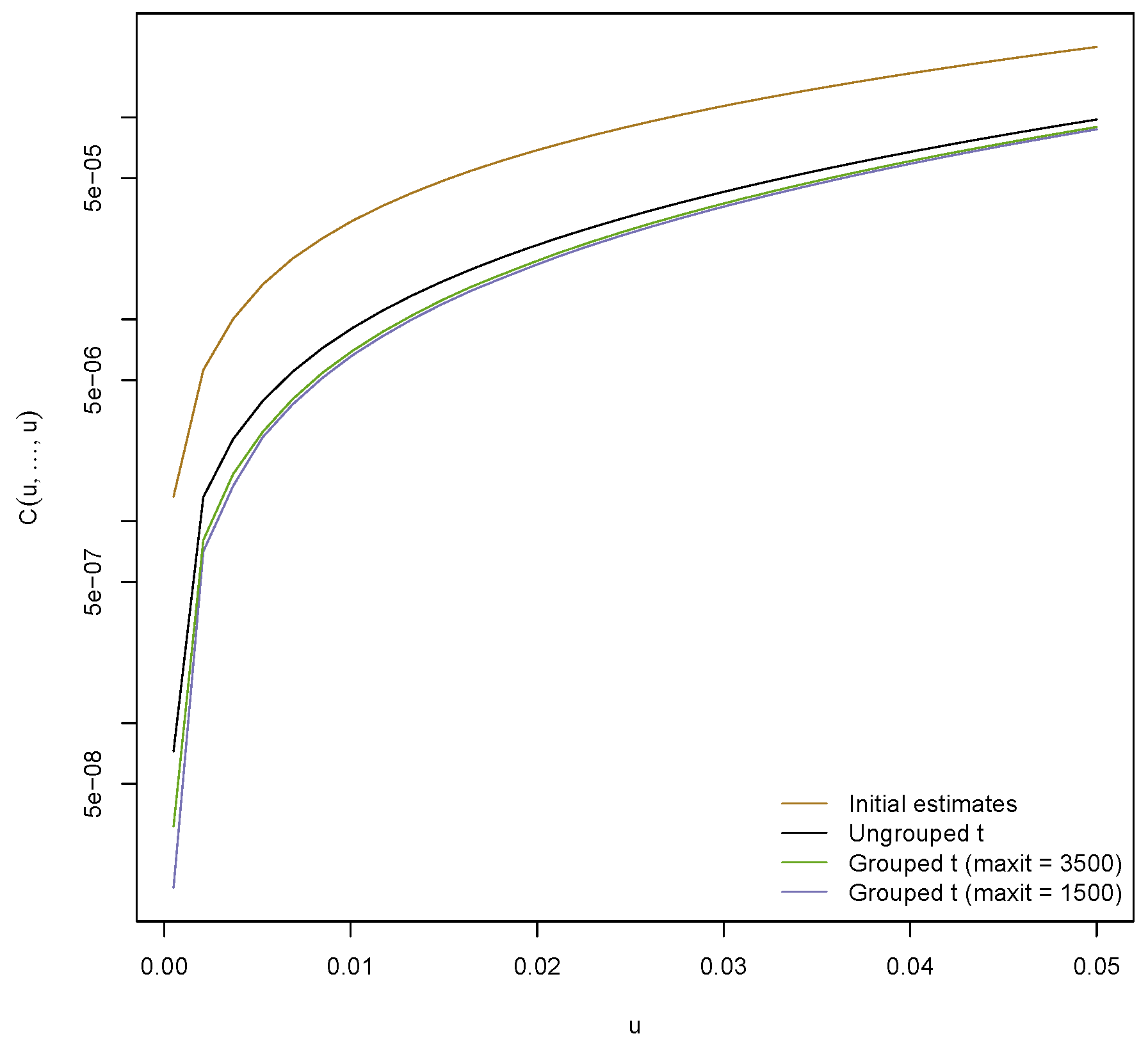
In order to examine the impact of the different estimates on the underlying copula in terms of its tail behavior, Figure 7 displays the probability $C(u,\dots ,u)$ estimated using methods from Section 6.3 as a function of u; in a risk management context, $C(u,\dots ,u)$ is the probability of a jointly large loss, hence a rare event. An absolute error tolerance of ${10}^{-7}$ was used to estimate the copula. The figure also includes the corresponding probability for the ungrouped t copula, for which the dof were estimated to be 6.3. Figure 7 indicates that the initial estimates yield the most heavy tailed model. This seems reasonable since all initial estimates for the dof range between 0.9 and 5.3 (with average 2.8). The models obtained from the MLEs exhibit the smallest tail probability, indicating that these are the least heavy tailed models considered here. This is in line with Figure 6, which shows that the dof are substantially larger than the initial estimates. The ungrouped t copula is more heavy tailed than the fitted grouped one (with MLEs) but less heavy tailed than the fitted grouped one with initial estimates.

This example demonstrates that it is generally advisable to estimate the dof jointly when grouped modeling is of interest, rather than group-wise as suggested in Daul et al. (2003). Indeed, in this particular example, the initial estimates give a model that substantially overestimates the risk of jointly large losses. As can be seen from Figure 6, optimizing an estimated log-likelihood function is not at all trivial, in particular when many parameters are involved. Indeed, the underlying optimizer never detected convergence, which is why the user needs to carefully assess which specification of maxit to use. We plan on exploring more elaborate optimization procedures which perform better in large dimensions for this problem in the future.

Example 3.

In this example, we consider the problem of mean-variance (MV) portfolio optimization in the classical Markowitz (1952) setting. Consider d assets, and denote by ${\mathit{\mu }}_t$ and ${\mathsf{\Sigma }}_t$ the expected return vector on the risky assets in excess of the risk free rate and the variance-covariance (VCV) matrix of asset returns in the portfolio at time t, respectively. We assume that an investor chooses the weights ${\mathit{x}}_t$ of the portfolio to maximize the quadratic utility function $U\left({\mathit{x}}_t\right)={\mathit{x}}_t^{\top }{\mathit{\mu }}_t-\frac{\gamma }{2}{\mathit{x}}_t^{\top }{\mathsf{\Sigma }}_t{\mathit{x}}_t$, where in what follows we assume the risk-aversion parameter $\gamma =1$. When there are no shortselling (or other) constraints, one finds the optimal ${\mathit{x}}_t$ as ${\mathit{x}}_t={\mathsf{\Sigma }}_t^{-1}{\mathit{\mu }}_t$. As in Low et al. (2016), we consider relative portfolio weights, which are thus given by

$${\mathit{w}}_t=\frac{{\mathsf{\Sigma }}_t^{-1}{\mathit{\mu }}_t}{|{\mathbf{1}}^{\top }{\mathsf{\Sigma }}_t^{-1}{\mathit{\mu }}_t|}.$$

As such, the investor needs to estimate ${\mathit{\mu }}_t$ and ${\mathsf{\Sigma }}_t$. If we assume no shortselling, i.e., $x_{t,j}\ge 0$ for $j=1,\dots ,d$, the optimization problem can be solved numerically, for instance using the R package quadprog of Turlach et al. (2019).

Assume we have return data for the d assets stored in vectors ${\mathit{y}}_t$, $t=1,\dots ,T$, and a sampling window $0<M<T$. We perform an experiment similar to Low et al. (2016) and compare a historical approach with a model-based approach to estimate ${\mathit{\mu }}_t$ and ${\mathsf{\Sigma }}_t$. The main steps are as follows:

1. 

In each period $t=M+1,\dots ,T$, estimate ${\mathit{\mu }}_t$ and ${\mathsf{\Sigma }}_t$ using the M previous return data ${\mathit{y}}_i$, $i=t-M,\dots ,t-1$.

2. 

Compute the optimal portfolio weights ${\mathit{w}}_t$ and the out-of-sample return $r_t={\mathit{w}}_t^{\top }{\mathit{y}}_t$.

In the historical approach, ${\mathit{\mu }}_t$ and ${\mathsf{\Sigma }}_t$ in the first step are merely computed as the sample mean vector and sample VCV matrix of the past return data. Our model-based approach is a simplification of the approach used in Low et al. (2016). In particular, to estimate ${\mathit{\mu }}_t$ and ${\mathsf{\Sigma }}_t$ in the first step, the following is done in each time period:

1a. 

Fit marginal $\mathit{ARMA}(1,1)-\mathit{GARCH}(1,1)$ models with standardized t innovations to ${\mathit{y}}_i$, $i=t-M,\dots ,t-1$.

1b. 

Extract the standardized residuals and fit a grouped t copula to the pseudo-observations thereof.

1c. 

Sample n vectors from the fitted copula, transform the margins by applying the quantile function of the respective standardized t distribution and based on these n d-dimensional residuals, sample from the fitted $\mathit{ARMA}(1,1)-\mathit{GARCH}(1,1)$ giving a total of n simulated return vectors, say ${\mathit{y}}_i^{\prime }$, $i=1,\dots ,n$.

1d. 

Estimate ${\mathit{\mu }}_t$ and ${\mathsf{\Sigma }}_t$ from ${\mathit{y}}_i^{\prime }$, $i=1,\dots ,n$.

The historical and model-based approaches each produce $T-M$ out-of-sample returns from which we can estimate the certainty-equivalent return (CER) and the Sharpe-ratio (SR) as

$$\widehat{\mathrm{CER}}={\widehat{\mu }}_r-\frac{1}{2}{\widehat{\sigma }}_r^2\mathrm{and}\widehat{\mathrm{SR}}=\frac{{\widehat{\mu }}_r}{{\widehat{\sigma }}_r},$$

where ${\widehat{\mu }}_r$ and ${\widehat{\sigma }}_r$ denote the sample mean and sample standard deviation of the $T-M$ out-of-sample returns; see also Tu and Zhou (2011). Note that larger, positive values of the SR and CER indicate better portfolio performance.

We consider logarithmic returns of the constituents of the Dow Jones 30 index from 1 January 2013 to 31 December 2014 ($n=503$ data points obtained from the R package qrmdata of Hofert and Hornik (2016)), a sampling window of $M=250$ days, $n={10}^4$ samples to estimate ${\mathit{\mu }}_t$ and ${\mathsf{\Sigma }}_t$ in the model-based approach, a risk-free interest rate of zero and no transaction costs. We report (in percent) the point estimates ${\widehat{\mu }}_r$, $\widehat{\mathrm{CER}}$ and $\widehat{\mathrm{SR}}$ for the historical approach and for the model-based approach based on an ungrouped and grouped t copula in

Table 2. Estimated returns, certainty-equivalent returns (CERs) and Sharpe-ratios (SRs) (all in percentage points) of a mean-variance (MV) investor under three investment rules assuming no short-sales: Model-based with grouped and ungrouped t copula and historical.

	${\widehat{\mathit{\mu }}}_{\mathit{r}}$	$\widehat{\mathbf{CER}}$	$\widehat{\mathbf{SR}}$
historical	0.045	0.041	5.356
ungrouped t	0.075	0.071	8.678
grouped t	0.083	0.079	9.474

assuming no shortselling. To limit the run time for this illustrative example, the degrees of freedom for the grouped and ungrouped t copula are estimated once and held fixed throughout all time periods $t=M+1,\dots ,T$. We see that the point estimates for the grouped model exceed the point estimates for the ungrouped model.

7. Discussion and Conclusions

We introduced the class of grouped normal variance mixtures and provided efficient algorithms to work with this class of distributions: Estimating the distribution function and log-density function, estimating the copula and its density, estimating Spearman’s rho and Kendall’s tau and estimating the parameters of a grouped NVM copula given a dataset. Most algorithms (and functions in the package nvmix) merely require one to provide the quantile function(s) of the mixing distributions. Due to their importance in practice, algorithms presented in this paper (and their implementation in the R package nvmix) are widely applicable in practice.

We saw that the distribution function (and hence, the copula) of grouped NVM distributions can be efficiently estimated even in high dimensions using RQMC algorithms. The density function of grouped NVM distributions is in general not available in closed form, not even for the grouped t distribution, so one relies on its estimation. Our proposed adaptive algorithm is capable of estimating the log-density even in high dimensions accurately and efficiently. Fitting grouped normal variance mixture copulas, such as the grouped t copula, to data is an important yet challenging task due to lack of a tractable density function. Thanks to our adaptive procedure for estimating the density, the parameters can be estimated jointly in the special case of a grouped t copula. As was demonstrated in the previous section, it is indeed advisable to estimate the dof jointly, as otherwise one might severely over- or underestimate the joint tails.

A computational challenge that we plan to further investigate is the optimization of the estimated log-likelihood function, which is currently slow and lacks a reliable convergence criterion that can be used for automation. Another avenue for future research is to study how one can, for a given multivariate dataset, assign the components to homogeneous groups.

8. Proofs

Proof of Proposition 1.

This is an immediate application of a proposition proven in (Daul et al. 2003, p. 6). □

Proof of Proposition 2.

Assume that $\mathsf{\Sigma }=P$ is a correlation matrix with $P_{12}=\rho$ (otherwise standardize the margins). We can write

$$\begin{array}{c}\hfill X_1=\sqrt{W_1}{Z}_1,X_2=\sqrt{W_2}\left(\rho Z_1+\sqrt{1-{\rho }^2}{Z}_2\right),\end{array}$$

where $\mathit{Z}=(Z_1,Z_2)\sim N_2(\mathbf{0},I_2)$ and $W_j=F_{W_j}^{\leftarrow }\left(U\right)$ for $j=1,2$ and $U\sim (0,1)$. Let $\mathit{S}=(S_1,S_2)\sim \mathrm{U}\left({\mathbb{S}}^{2-1}\right)$ be uniformly distributed on the unit circle. Such random vector $\mathit{S}$ can be expressed via the stochastic representation

$$\begin{array}{c}\hfill S_1=cos\left(\mathsf{\Theta }\right),S_2=sin\left(\mathsf{\Theta }\right),\mathsf{\Theta }\sim \left([-\pi ,\pi )\right).\end{array}$$

Note that $\mathit{Z}/\sqrt{{\mathit{Z}}^{\top }\mathit{Z}}\sim \mathrm{U}\left({\mathbb{S}}^{2-1}\right)$ is independent of ${\mathit{Z}}^{\top }\mathit{Z}\sim {\chi }_2^2$. Let $W_3^2\sim {\chi }_2^2$ be independent of $\mathit{S}$, $W_1$, $W_2$ and set $W_j^{\prime }=\sqrt{W_j}{W}_3$ for $j=1,2$. Then

$$\begin{array}{c}\hfill X_1=W_1^{\prime }{S}_1=W_1^{\prime }cos\left(\mathsf{\Theta }\right),X_2=W_2^{\prime }\left(\rho S_1+\sqrt{1-{\rho }^2}{S}_2\right)=W_2^{\prime }\left(\rho cos\left(\mathsf{\Theta }\right)+\sqrt{1-{\rho }^2}sin\left(\mathsf{\Theta }\right)\right).\end{array}$$

Finally, setting $\varphi =arcsin\rho$ and noting that $\mathbb{P}(W_j^{\prime }>0)=1$ for $j=1,2$ allows us to compute $\mathbb{P}(X_1>0,X_2>0)$ via

$$\begin{array}{cc}\hfill & \phantom{=}\mathbb{P}(X_1>0,X_2>0)=\mathbb{P}\left(W_1^{\prime }cos\left(\mathsf{\Theta }\right)>0,W_2^{\prime }\left(\rho cos\left(\mathsf{\Theta }\right)+\sqrt{1-{\rho }^2}sin\left(\mathsf{\Theta }\right)\right)>0\right)\hfill \\ \hfill & =\mathbb{P}\left(cos\left(\mathsf{\Theta }\right)>0,sin\left(\varphi \right)cos\left(\mathsf{\Theta }\right)+cos\left(\varphi \right)sin\left(\mathsf{\Theta }\right)>0\right)=\mathbb{P}\left(cos\left(\mathsf{\Theta }\right)>0,sin(\mathsf{\Theta }+\varphi )>0\right)\hfill \\ \hfill & =\mathbb{P}\left(\mathsf{\Theta }\in (-\pi /2,\pi /2)\cap (-\varphi ,\pi -\varphi )\right)=\frac{\pi /2+\varphi }{2\pi }.\hfill \end{array}$$

Substituting $\varphi =arcsin\left(\rho \right)$ gives the result. □

Proof of Proposition 3.

We follow (McNeil et al. 2015, Proposition 7.44), where a similar result was shown for $\mathit{X}\sim {\mathrm{NVM}}_2(\mathit{\mu },\mathsf{\Sigma },F_W)$. Since $\mathit{X}$ has continuous margins, we can write

$$\begin{array}{c}\hfill {\rho }_{\mathrm{S}}(X_1,X_2)=6\mathbb{P}((X_1-{\tilde{X}}_1)(X_2-{\overline{X}}_2)>0)-3,\end{array}$$

(31)

where ${\tilde{X}}_1$ and ${\overline{X}}_2$ are random variables with ${\tilde{X}}_1\underset{}{\stackrel{\mathrm{d}}{=}}{X}_1$ and ${\overline{X}}_2\underset{}{\stackrel{\mathrm{d}}{=}}{X}_2$ and where $(X_1,X_2)$, ${\tilde{X}}_1$ and ${\overline{X}}_2$ are all independent; see (McNeil et al. 2015, Proposition 7.34).

Let $W_j=F_{W_j}^{\leftarrow }\left(U\right)$ for $j=1,2$, ${\tilde{W}}_1=F_{W_1}^{\leftarrow }\left(\tilde{U}\right)$ and ${\overline{W}}_2=F_{W_2}^{\leftarrow }\left(\overline{U}\right)$ for $U,\tilde{U},\overline{U}\underset{}{\stackrel{\mathrm{ind}.}{\sim }}\mathrm{U}(0,1)$. Furthermore, let $\tilde{Z},\overline{Z}\underset{}{\stackrel{\mathrm{ind}.}{\sim }}N(0,1)$, independent of $\mathit{Z}\sim N_2(0,P)$. Finally, set

$$\begin{array}{c}\hfill X_1=\sqrt{W_1}{Z}_1,X_2=\sqrt{W_2}{Z}_2,\tilde{X}=\sqrt{{\tilde{W}}_1}\tilde{Z},\overline{X}=\sqrt{{\overline{W}}_2}\overline{Z}.\end{array}$$

and define the random vector $\mathit{Y}=(Y_1,Y_2)$ via

$$\begin{array}{c}\hfill Y_1=X_1-\tilde{X}=\sqrt{W_1}{Z}_1-\sqrt{{\tilde{W}}_1}\tilde{Z},Y_2=X_2-\overline{X}=\sqrt{W_2}{Z}_2-\sqrt{{\overline{W}}_2}\overline{Z}.\end{array}$$

From (31) it follows that we need to compute $\mathbb{P}(Y_1{Y}_2>0)$. Conditional on $U,\tilde{U},\overline{U}$, we find

$$\begin{array}{c}\hfill \mathit{Y}\mid U,\tilde{U},\overline{U}\sim N_2\left(0,\left(\begin{array}{cc}{W}_1+{\tilde{W}}_1& \sqrt{W_1{W}_2}\rho \\ \sqrt{W_1{W}_2}\rho & W_2+{\overline{W}}_2\end{array}\right)\right).\end{array}$$

Since the multivariate normal distribution is a special case of a gNVM distribution (obtained with $W_1=\dots =W_d=c$ for some $c>0$), Proposition 2 can be applied to compute

$$\begin{array}{cc}\hfill {\rho }_{\mathrm{S}}(X_1,X_2)& =6\mathbb{P}\left((X_1-{\tilde{X}}_1)(X_2-{\overline{X}}_2)>0\right)-3=3\left(\mathbb{E}\left(2\mathbb{P}(Y_1{Y}_2>0\mid U,\tilde{U},\overline{U})\right)-1\right)\hfill \\ \hfill & =3\left(\mathbb{E}\left(4\mathbb{P}(Y_1>0,Y_2>0\mid U,\tilde{U},\overline{U})\right)-1\right)\hfill \\ \hfill & =\frac{6}{\pi }\mathbb{E}\left(arcsin\left(\rho \sqrt{\frac{F_{W_1}^{\leftarrow }\left(U\right)F_{W_2}^{\leftarrow }\left(U\right)}{(F_{W_1}^{\leftarrow }\left(U\right)+F_{W_1}^{\leftarrow }\left(\tilde{U}\right))(F_{W_2}^{\leftarrow }\left(U\right)+F_{W_2}^{\leftarrow }\left(\overline{U}\right))}}\right)\right).\hfill \end{array}$$

 □

Proof of Proposition 4.

For $u,q\in (0,1)$, let $x_j(u,q)=F_j^{\leftarrow }\left(q\right)/\sqrt{F_{W_j}^{\leftarrow }\left(u\right)}$ for $j=1,2$. Writing C instead of $C_{P,F_{\mathit{W}}}^{\mathrm{gNVM}}$ and ${\mathsf{\Phi }}_{\rho }$ for the distribution function of $\mathit{Z}\sim N_2(\mathbf{0},P)$, we get $C(q,q)={\int }_0^1{\mathsf{\Phi }}_{\rho }(x_1(u,q),x_2(u,q))\mathrm{d}u,$ which implies that

$$\begin{array}{c}\hfill \lambda =\underset{q\to 0^{+}}{lim}\frac{1}{q}C(q,q)=\underset{q\to 0^{+}}{lim}\frac{\partial }{\partial q}{\int }_0^1{\mathsf{\Phi }}_{\rho }\left(x_1(u,q),x_2(u,q)\right)\mathrm{d}u.\end{array}$$

Taking the derivative with respect to q gives

$$\begin{array}{c}\hfill \frac{\partial }{\partial q}{\int }_0^1{\mathsf{\Phi }}_{\rho }\left(x_1(u,q),x_2(u,q)\right)\mathrm{d}u={\int }_0^1\frac{\partial {\mathsf{\Phi }}_{\rho }}{\partial x_1}\frac{\partial x_1}{\partial q}\mathrm{d}u+{\int }_0^1\frac{\partial {\mathsf{\Phi }}_{\rho }}{\partial x_2}\frac{\partial x_2}{\partial q}\mathrm{d}u.\end{array}$$

(32)

We find $\frac{\partial x_i}{\partial q}={\left(\sqrt{F_{W_i}^{\leftarrow }\left(u\right)}{f}_i\left(F_i^{\leftarrow }\left(q\right)\right)\right)}^{-1}$ for $i=1,2$. Furthermore,

$$\begin{array}{c}\hfill \frac{\partial }{\partial x_1}{\mathsf{\Phi }}_{\rho }(x_1,x_2)=\frac{\partial }{\partial x_1}\mathbb{P}(Z_1\le x_1,Z_2\le x_2)=\varphi \left(x_1\right)\mathbb{P}(Z_2\le x_2\mid Z_1=x_1)=\varphi \left(x_1\right)\mathsf{\Phi }\left(\frac{x_2-\rho x_1}{\sqrt{1-{\rho }^2}}\right);\end{array}$$

the derivative $\frac{\partial }{\partial x_2}{\mathsf{\Phi }}_{\rho }(x_1,x_2)$ can be found analogously by swapping the roles of $Z_1$ and $Z_2$. Plugging the derivatives into (32) and taking the limit gives the result in the statement. □