Modeling County-Level Spatio-Temporal Mortality Rates Using Dynamic Linear Models

Abstract

The lifestyles and backgrounds of individuals across the United States differ widely. Some of these differences are easily measurable (ethnicity, age, income, etc.) while others are not (stress levels, empathy, diet, exercise, etc.). Though every person is unique, individuals living closer together likely have more similar lifestyles than individuals living hundreds of miles apart. Because lifestyle and environmental factors contribute to mortality, spatial correlation may be an important feature in mortality modeling. However, many of the current mortality models fail to account for spatial relationships. This paper introduces spatio-temporal trends into traditional mortality modeling using Bayesian hierarchical models with conditional auto-regressive (CAR) priors. We show that these priors, commonly used for areal data, are appropriate for modeling county-level spatial trends in mortality data covering the contiguous United States. We find that mortality rates of neighboring counties are highly correlated. Additionally, we find that mortality improvement or deterioration trends between neighboring counties are also highly correlated.

1. Introduction

There has long been significant interest in the modeling and projection of human mortality trends over time. Prior to the last 30 years or so, this modeling was typically done in a deterministic manner, using methods like extrapolation, or fitting one-factor (age) or two-factor (age, year) models to historical trends. See Dickson et al. (2020) for a development of these deterministic factor-based mortality improvement methods.

More recently, stochastic methods of modeling the changes in mortality have become the standard for researchers and practitioners. Stochastic mortality models have several advantages over their deterministic counterparts. First, the recognition that the processes underlying mortality rates are themselves stochastic leads to the tendency of stochastic models to be inherently more realistic than deterministic ones (Cairns et al. 2009). In addition, there are also practical reasons to favor stochastic models, one of the most important being that they better allow us to assess uncertainty in our projections, whether this uncertainty is due to model risk, parameter uncertainty, or the inherent randomness of the process.

One of the earlier stochastic mortality models, and certainly among the most widely used, was the Lee–Carter model (Lee and Carter 1992). While this model has some notable advantages such as simplicity and interpretability of model parameters, it also suffers from several disadvantages including poor fits to some data sets, a lack of smoothness across ages, and the fact that it ignores age-time interactions, thus preventing the modeling of cohort effects commonly found in population mortality data sets.

Many researchers have offered variations on the Lee–Carter model that seek to address some of these shortcomings; the Cairns–Blake–Dowd model (Cairns et al. 2006) and its extensions have been widely utilized to model mortality improvements. For a discussion of the properties and a quantitative comparison of the Lee–Carter and Cairns–Blake–Dowd models and variants, the reader is referred to Cairns et al. (2009); Booth and Tickle (2008) offers a broad review of mortality forecasting methodologies, including Lee–Carter and its extensions, as well as older deterministic methods.

One potentially significant component missing from the above models is the recognition of potential spatial (geographic) correlations within mortality data. It seems plausible that mortality trends in neighboring locations might share more similar characteristics than those corresponding to well-separated locations, and that incorporating a spatial component into our mortality model might help strengthen and improve our understanding and projection of mortality trends. We might also desire our models to include the possibility of space-time interactions.

Many researchers have indeed incorporated spatial and/or spatio-temporal effects into mortality models, with Bayesian and empirical Bayes approaches having become popular. Bayesian approaches allow for the incorporation of prior structural knowledge into the model, and developments in both computing capability and methodologies have allowed for the efficient production of the requisite samples from the desired posterior distribution. Some early examples utilizing empirical Bayes approaches to account for spatial effects include Bernardinelli and Montomoli (1992); Clayton and Kaldor (1987); Manton et al. (1989) reviews empirical Bayes and fully Bayesian approaches to modeling spatial variations in mortality rates.

Waller et al. (1997) expanded existing spatial modeling by using a hierarchical Bayesian approach which allowed for spatial and temporal effects, as well as spatio-temporal interactions; they applied their model to county-level lung cancer death rates in the state of Ohio. Xia and Carlin (1998) analyzed this same data set using similar methods and adding in the effects of covariates thought to be relevant, such as age and smoking prevalence.

More recently, Ayele et al. (2015) used a structured additive logistic regression model to describe the mortality rates for young children in Ethiopia. This study utilized a Gaussian Markov random field to account for prior knowledge of spatial effects. Dwyer-Lindgren et al. (2016) used a Bayesian approach to fit a hierarchical model which allowed for spatial effects between neighboring counties, with covariates also being measured at the county level.

Alexander et al. (2017) used a Bayesian hierarchical model to obtain subnational mortality estimates, in order to better understand intra-national health inequalities. They applied their model to simulated data from the United States, as well as actual data from France, broken into 19 age groups. Their model used the first three principal components from some set of standard mortality curves, with a random effect to account for potential overdispersion. Their model achieved geographic pooling by using a common distribution centered on the state or country means. This model also imposed smoothness across time by incorporating information from the previous two time periods. They found that the resulting model fit better than simpler models, particularly in areas with smaller populations; this was notable because small populations often lead to higher variances in the respective mortality estimates.

We add spatio-temporal interactions directly into the mortality model using a conditional auto-regressive (CAR) model (Besag et al. 1991). A CAR model is specifically designed for spatial data that is collected into geographic regions, such as county data (Cressie 2015) and has been extended to spatio-temporal data through various means (Alegana et al. 2013; Martínez-Beneito et al. 2008). Temporal variations in mortality will be accounted for using a spatially-varying linear time trend (Bernardinelli et al. 1995). The resulting model will show both general mortality rates across the United States as well as region specific mortality improvement over time.

The remainder of this paper is organized as follows: Section 2 describes the mortality and covariate data we use in our study; Section 3 introduces the CAR model we use to describe the mortality data, including the Bayesian priors and resulting posterior distributions; Section 4 presents the results of the study and discusses the major findings; Section 5 concludes the paper with a discussion of the implications of the study and ideas for further research.

2. Data

The data used in this analysis were sourced from the Division of Vital Statistics of the National Center for Health Statistics (NCHS) which is a part of the Centers for Disease Control and Prevention (CDC). The data contain demographic and mortality information for each of the individuals who died in the United States between the years 2000 and 2017. For this analysis, we study the mortality rates by year, age, sex, and county of residence.

The exposures for each demographic group are obtained through population estimates published by the United States Census Bureau. The annual population estimates are based on the most recent decennial census and then adjusted for births, deaths, and migrations (see U.S. Census Bureau (2020) for more detailed information). The census data set bins ages into eighteen five-year age groups starting with ages 0–4 and ending with ages 85+ as the 18th age group. We also bin our data according to these age groups. Separate statistical models are fit for every age group and sex combination, for a total of 36 models.

We made several modifications to make the data suitable for spatio-temporal models. Some counties in the data set had population estimates of zero for one or more age groups. Additionally, a small number of low-population counties had death totals that marginally exceeded exposure levels for one or more age groups. These counties were combined with the neighboring county with the largest population. By choosing the neighboring county with the largest population we were able to maintain spatial relationships while minimizing disruption to the empirical mortality rate. Note that in this paper we will use the term “county” to refer to geographic subdivisions of a state, even in the state of Louisiana, which is divided into parishes.

During the course of the 18 years of study, some county names were changed and some boundaries were adjusted. To maintain consistency, the data were adjusted to match the county names and boundaries in 2017. A full list of counties that were adjusted are in Appendix A. Neighboring counties were defined using the county adjacency file published by the United States Census Bureau. Observations for counties in Alaska, Hawaii, and the U.S. territories were excluded from the analysis as their relative isolation makes it difficult to establish spatial correlation.

After combining counties with extremely small populations, accounting for county changes, and removing counties outside of the contiguous United States, our data contained a total of 3092 counties for study. The number of resident deaths in the continental U.S. between years 2000 and 2017 was 45,036,799.

Using the county-level population estimates, we calculated the empirical mortality rate for 55–59 year-old females for each county in 2010, as shown in Figure 1. The choropleth shows potential spatial correlation. For example, mortality rates appear to be higher in the South and lower in the Midwest. Similar correlations are visible for different age groups, years, and sex combinations. This supports our assertions that nearby counties likely have similar characteristics, and this correlation should be accounted for in a statistical model.

The spatial correlation that seems to be present in the majority of age groups tends to subside with the oldest age group (85 years or older). Figure 2 shows a choropleth with the empirical mortality rates for females 85 years or older in 2010. While some spatial correlation is still likely present, the choropleth shows greater variation in mortality rates between neighboring counties than seen in the choropleths for younger age groups.

Figure 3 displays the mortality trends over time for each age group and sex combination averaged over every county. The plots show that, in general, mortality rates have decreased over time. While it does appear that there has been an increase in mortality for some of the lower age groups, it is important to keep in mind that the scale represents very small changes in mortality, and the increases seen may be a result of a leveling of the mortality rate, rather than an increasing trend. Regardless, the changes in mortality rate over time make it important to include both temporal and spatial components in the models. Figure 3 also shows that empirical death rates are higher for males than females for most age group and year combinations. These differences contributed to the decision to build separate models for female and male mortality rates.

Several covariates, such as unemployment rate, race, education, marital status, and income, were considered for inclusion in the model. Unfortunately, the availability of county-level data for each year is limited due to privacy laws. We found the data that are only available, for example, on census years or at a state level do not provide enough information to reasonably perform stable sampling from the posterior. The only covariate for which we found reputable county-level estimates for each year from 2000 to 2017 was unemployment rate, as provided by the U.S. Bureau of Labor Statistics. Therefore, for the models in this paper we include unemployment rate as the only explanatory variable. In future research, we hope to obtain yearly county-level data for other explanatory variables or make model-based adjustments in an effort to accurately estimate them.

Though the unemployment data released by the U.S. Bureau of Labor Statistics are nearly complete, unemployment rates were unavailable for seven counties in Louisiana in 2005 and 2006 (see Appendix B). These counties correspond to the areas that were most severely impacted by Hurricane Katrina. While unemployment rates were likely higher in these areas than in other parts of the state, due to the lack of data we simply imputed the missing values using the average of the other Louisiana counties’ unemployment rates in both years. Though the imputed values may not accurately reflect the true unemployment rates in these areas, the small number of imputed values will not substantially affect the model fit.

The choropleth map in Figure 4 shows the unemployment rates by county in 2010. This map shows clear spatial correlation between areas. For example, there is high unemployment on the coasts, whereas unemployment is lower in the center of the United States.

To explore potential trends in unemployment rate over time, we calculated the average county unemployment rate weighted by county population. The results are seen in Figure 5. The plot shows fluctuation in the unemployment rate corresponding to periods of economic downturn and growth.

3. Methods

This section outlines the methodology for the CAR model that will be used to model the mortality data.

3.1. Bayesian Binomial Hierarchical Model

Let $\mathbf{Y}$ be the vector of data points where $y_{kt}$ represents the data point at location k, where $k=1,2,\cdots ,K$, and time t, where $t=1,2,\cdots ,T$. The data is in terms of the number of deaths in each region and at each time point. The total population for each region at each time is also known, so the most appropriate likelihood for this data set is binomial, $y_{kt}\sim \mathrm{Binomial}(m_{kt},{\theta }_{kt})$, where $m_{kt}$ is the total population and ${\theta }_{kt}$ is the probability of death.

We achieve this likelihood through a logistic link function on the probability of death,

$$log\left({\theta }_{kt}/(1-{\theta }_{kt})\right)={\mathbf{x}}_{kt}^{\prime }\beta +{\psi }_{kt}.$$

(1)

The vector ${\mathbf{x}}_{kt}$ represents covariate information for location k at time t and $\beta$ contains the corresponding coefficients. The term ${\psi }_{kt}$ collects all the spatial and temporal random effects that create the spatio-temporal dependence. This approach of separating fixed and random effects and using a link function to relate these effects to the likelihood is common in spatial data analysis (Cressie and Wikle 2015; Diggle et al. 1998) and can be seen in Paciorek (2007) specifically using the binomial likelihood.

3.2. Conditional Auto-Regressive Priors

All spatio-temporal models assume that observations closer together in time and space are more highly correlated than observations farther apart. The time component of the mortality data is measured in years, which provides a straightforward way of defining distance. Counties, however, have odd shapes and do not provide an intuitive distance measurement.

To model spatial dependence we use the concept of a neighborhood structure, where two counties that share any portion of a border are considered first-order neighbors. An adjacency matrix W can be built where $W_{kj}$ is 1 if locations k and j are neighbors and 0 otherwise.

Let $\mathbf{\varphi }=({\varphi }_1,\cdots ,{\varphi }_K)$ be a spatially dependent random vector. A conditional auto-regressive (CAR) prior is built on the idea that the expected value of the random effect at a specific location can be defined as a linear combination of its neighbors, through the relationship

$${\varphi }_k|{\varphi }_{\left(k\right)}\sim N\left(\rho \sum _{j=1}^K\frac{1}{N_k}{W}_{kj}{\varphi }_j,{\tau }^2\right)$$

where ${\varphi }_{\left(k\right)}$ represents all locations excluding location k and $N_k$ is the total number of neighbors for location k. The degree of dependence between neighbors is captured by $\rho$, where a larger value signifies a stronger dependence.

This structure results in an overall distribution for the random vector to be

$$\mathbf{\varphi }\sim {\mathrm{N}}_{\mathrm{K}}\left(\mathbf{0},{\tau }^2{(D-\rho W)}^{-1}\right),$$

(2)

where $D=\mathrm{diag}(N_1,\cdots ,N_K)$ is a diagonal matrix collecting the number of neighbors for each location and $\mathbf{0}$ is a vector of 0s.

3.3. CAR Linear Model

When discussing the model structure, we will focus on the random effects ${\psi }_{kt}$ in Equation (1). The CAR linear model structure is

$${\psi }_{kt}={\varphi }_k+(\alpha +{\delta }_k)\frac{t-\overline{t}}{T}.$$

(3)

The term ${\varphi }_k$ is given a CAR prior according to Equation (2) and represents a standard spatial random effect. This model assumes a linear trend in the random effect over time with a slope equal to $\frac{\alpha +{\delta }_k}{T}$, suggesting that the amount of mortality change over time is region-specific. The term ${\delta }_k$ is also given a CAR prior.

The neighborhood structures will be the same between the two spatial effects, but the variance ${\tau }^2$ and dependence parameter $\rho$ will be different, leading to specific priors of $\mathbf{\varphi }\sim N_K\left(0,{\tau }_s^2{(D-{\rho }_{s}W)}^{-1}\right)$ and $\mathbf{\delta }\sim N_K\left(0,{\tau }_t^2{(D-{\rho }_{t}W)}^{-1}\right)$ where $\mathbf{\varphi }={({\varphi }_1,\cdots ,{\varphi }_K)}^{\prime }$ and $\mathbf{\delta }={({\delta }_1,\cdots ,{\delta }_K)}^{\prime }$. Both $\mathbf{\varphi }$ and $\mathbf{\delta }$ will have constraints that they must sum to 0, a method known as conditioning via kriging (Cressie 2015). This will allow the intercept term in the fixed effects to represent the overall average mortality (on the logistic scale) for all times and spatial locations. Furthermore, the term $\alpha$ will represent the average slope for the linear mortality trend for all locations.

3.4. Posterior Simulation

Combining all the information introduced for the specific model components as well as the prior information for all parameters, the full Bayesian CAR Spatio-temporal Model we are using is

$$\begin{array}{ccc}\hfill y_{kt}& \sim & \mathrm{Binomial}(m_{kt},{\theta }_{kt}),k=1,\cdots ,K;t=1,\cdots ,T\hfill \\ \hfill log\left({\theta }_{kt}/(1-{\theta }_{kt})\right)& =& {\mathbf{x}}_{kt}^{\prime }\mathbf{\beta }+{\psi }_{kt}\hfill \\ \hfill {\psi }_{kt}& =& {\varphi }_k+(\alpha +{\delta }_k)\frac{t-\overline{t}}{T}\hfill \\ \hfill \mathbf{\varphi }& \sim & N_K\left(\mathbf{0},{\tau }_s^2{(D-{\rho }_{s}W)}^{-1}\right)\hfill \\ \hfill \mathbf{\delta }& \sim & N_K\left(\mathbf{0},{\tau }_t^2{(D-{\rho }_{t}W)}^{-1}\right)\hfill \\ \hfill {\tau }_t^2,{\tau }_s^2& \sim & IG(1,0.01),{\rho }_t,{\rho }_s\sim \mathrm{Uniform}(0,1)\hfill \\ \hfill \alpha & \sim & N\left(0,1000\right),\mathbf{\beta }\sim N_r({\mathbf{0}}_r,{\mathit{I}}_r)\hfill \end{array}$$

where IG refers to the Inverse Gamma distribution and r is equal to the dimension of $\mathbf{\beta }$.

This full model description can define a likelihood that will be leveraged in simulating draws from the posterior distribution of the parameters. For nearly all the parameters, posterior samples will be drawn using Metropolis–Hastings with Gibbs sampling (Neal 1993). The proposal distributions are all Gaussian random walks with tuning parameters found such that all acceptance rates are between 40% and 50% for the scalar parameters $\alpha$, ${\rho }_s$, ${\rho }_t$ and $\mathbf{\beta }$ and acceptance rates are between 20% and 40% for the vectors $\mathbf{\varphi }$ and $\mathbf{\delta }$.

The only parameters that have closed form posterior distributions are the variance terms ${\tau }_s^2$ and ${\tau }_t^2$. The posterior distribution for ${\tau }_s^2$ and ${\tau }_t^2$ given the other parameters will be

$${\tau }_s^2|·\sim \mathrm{IG}\left(a+1/2,b+{\mathbf{\varphi }}^{\prime }(D-{\rho }_{s}W)\mathbf{\varphi }/2\right),$$

$${\tau }_t^2|·\sim \mathrm{IG}\left(a+1/2,b+{\mathbf{\varphi }}^{\prime }(D-{\rho }_{t}W)\mathbf{\varphi }/2\right).$$

4. Results

The model in Section 3.4 was fit using the mortality data described in Section 2. With unemployment as the only regressor, the fixed effects in the model are ${\mathbf{x}}_{kt}^{\prime }\mathbf{\beta }={\beta }_0+{\beta }_{1}Unem{p}_{kt},$ where $Unem{p}_{kt}$ represents the unemployment in county k and time t. The priors for ${\tau }_t^2$ and ${\tau }_s^2$ were chosen to be relatively uninformative with the shape parameter equal to 1 and the rate parameter equal to 0.01. The prior for $\mathbf{\beta }$ was chosen so that ${\mathbf{\mu }}_{\beta }=\mathbf{0}$ and ${\Sigma }_{\beta }=\mathit{I}$. Additionally, the mean and variance of the prior distribution for $\alpha$ are ${\mu }_{\alpha }=0$ and ${\sigma }_{\alpha }^2=1000$, respectively. The model was run entirely using the CARBayesST package from the Comprehensive R Archive Network repository (Lee et al. 2018). The computation uses R for the MCMC steps although computationally intensive components were calculated using C++ via Rcpp (Eddelbuettel et al. 2011). An appropriate burn-in and overall convergence was checked using Geweke test statistics (Geweke 1992) as well as visual analysis of the trace plots. The number of samples drawn from the posterior was enough to give a reasonably large effective sample size.

All the effects we discuss and explore visually will be done in the logit scale as values on the untransformed scale are difficult to distinguish. Figure 6 shows the estimates and 95% credible intervals for the intercept, ${\beta }_0$, by age and sex. The narrow widths of the credible intervals in Figure 6 are difficult to distinguish from the point estimates. As the age categories are collected on intervals, the plots are simplified by using the lowest value in each age range. In this plot, and all subsequent plots, it is important to remember that we fit 36 models (one for each combination of age group and sex). These estimates are connected linearly for visualization purposes only. The shape of the graph follows the general trend of mortality rates such that mortality decreases after birth for a few years, and then continues to increase with age.

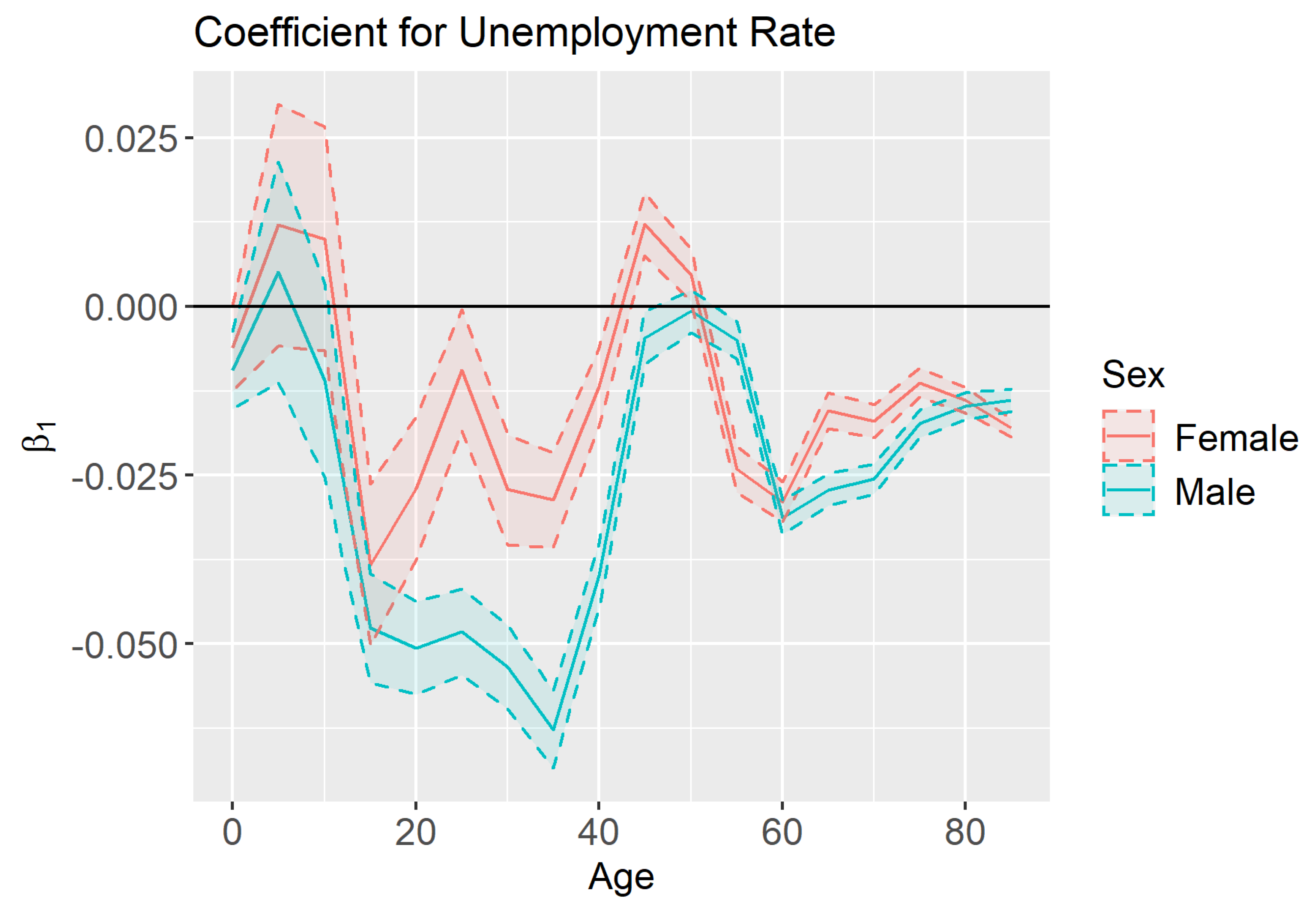
The estimates and credible intervals for the unemployment effect (${\beta }_1$) are shown in Figure 7. The wide credible intervals associated with the youngest age groups include zero, suggesting that there is little to no effect of county unemployment rate on the mortality rate of newborns and young children. However, once the children reach their teenage years an increase in unemployment rates is usually correlated with a decrease in mortality rates. This result may seem counterintuitive since research has shown that unemployment is correlated with an increase in mortality at an individual level (Gerdtham and Johannesson 2003). However, other studies corroborate our finding that in aggregate there is a negative correlation between a population’s unemployment and mortality rates (Ionides et al. 2013). Because our analysis only studies mortality rates in aggregate, we cannot comment on the effect of unemployment at an individual level. The magnitude of the unemployment rate effect is greater for young-adult males than young-adult females. However, the difference between the sexes tends to subside in later years. Overall, the estimated effect magnitudes were highest for young adults, while the effect of unemployment rate on mortality is minimal after retirement age.

Recall that the model in Section 3.4 assumes a linear time trend such that the parameter $\alpha$ represents the country-wide time trend and $\alpha +{\delta }_k$ represents the time trend for county k. Figure 8 shows the estimates and 95% credible intervals for $\alpha$ by age and sex. For the youngest age groups, as well as the older age groups, we see significant mortality improvement. This improvement is greater for the youngest age groups than the oldest ones. For young and middle-aged adults, we see deterioration in mortality. This deterioration could be attributed to the “deaths of despair” that are commonly mentioned in recent literature (Scutchfield and Keck 2017). Males ages 40–50 did experience some modest mortality improvement, but their mortality rates were already higher than the females of similar ages who experienced mortality deterioration.

To visualize the values $\alpha +{\delta }_k$ we plot them on a map of the United States. Negative values indicate mortality rates are decreasing which suggests mortality improvement over time while positive values indicate that mortality rates are increasing. Figure 9 shows these county-level time trends for females ages 55–59. The plot shows spatial correlation in time trends. For example, mortality rates seem to be increasing the most in the South, whereas there is general mortality improvement in Northeastern counties.

The magnitude of the spatial dependence in the time trend is governed by ${\rho }_t$. This implies that larger values of ${\rho }_t$ results in neighbors being more similar in terms of mortality improvement. Figure 10 shows that ${\rho }_t$ is close to one for most age groups, although it is much lower for children, teenagers, and individuals over 85 than it is for other age groups. The lower correlation may be visualized in Figure 11, where the correlation in the time trend between neighboring counties for females ages 15–19 is much less obvious than it is for females ages 55–59 as seen in Figure 9.

Similar trends were also seen in the spatial dependence parameter ${\rho }_s$, which represents the magnitude of the dependence in overall mortality between neighboring counties. The estimates and 95% credible intervals for ${\rho }_s$ are shown in Figure 12. Here we see that the spatial correlation is very low for 20–24 year olds of both sexes, as well as for individuals over 85. Notice, however, that the uncertainty in our estimates is much lower for the spatial dependence parameters than the temporal dependence parameters.

5. Conclusions

By using conditional auto-regressive priors, we incorporated spatio-temporal random effects into a stochastic mortality model. The large estimated spatial correlation values as well as the visual evidence support that these spatially correlated effects were important to the model, both in terms of overall mortality as well as mortality improvement. This borrowing of information across space and time improves model fit and will lead to more accurate estimates of trends and covariate effects.

The model used in this paper can be extended in a number of ways. A non-linear mortality time trend may be more appropriate, especially for a longer-term analysis. Additional covariates for which yearly and county-level data is not available can be included using geo-additive effects. Furthermore, the age groups can be modeled together in a multivariate model. These extensions and others will be considered in future work.