Geological Feature Modeling and Reserve Estimation of Uranium Deposits Based on Multiple Interpolation Methods

Abstract

Uranium resource distribution and accurate reserve evaluation are important references for mineral investment and production. Eight kinds of interpolation methods in the Groundwater Modeling System (GMS), including ordinary kriging (OK), are used in this study to predict the spatial distribution of reserve-related parameters, such as uranium grade, ore thickness and uranium content per square meter. The present study draws the following conclusions: (1) Cross-validation found that the uranium grade value using the spherical method is the closest to the actual value. The spherical method has the best interpolation effect. (2) The relative error, which is +3.62%, between the uranium reserves that is calculated by the spherical interpolation method and that by the traditional calculation value is the smallest. (3) The setting of the number of interpolation grids is related to the actual number of boreholes. The ratio between the two will affect the accuracy of reserve estimation, and different interpolation methods have different degrees of influence on reserve estimation. This method is applicable to all in-situ leaching sandstone uranium mines. Further study needs to be carried out toward heterogeneity of three-dimensional space, which will make the estimation more accurate.

1. Introduction

Economic evaluation of the mineral deposits is an important factor in deciding to open or invest in new mines [1]. Reliable reserve and grade estimation determine the economic evaluation of the mineral deposits. Uranium reserves need to be estimated in the stages of exploration, development, leaching and later environmental remediation [2]. Accurate prediction affects short-term and long-term production planning and can save economic costs.

Due to geological complexities of uranium ore formation and particularity of mining methods, estimation of uranium reserves is one of the problems faced by geologists and mining engineers [3,4,5,6,7,8,9,10,11]. At present, estimation of uranium reserves in China mainly include the geometric figure method, SD method and geostatistic method [12]. As a traditional method, based on geometric calculation, the geometric figure method uses different calculations according to volume of ore body, mainly including the section method, geological block method, polygon method and triangle method [13]. However, results of this are of low accuracy, and the calculation is complicated and inconvenient for computer technology. The SD method, an abbreviation for SD reserve calculation and verification method, has been developed independently by China and is suitable for China’s national conditions. Based on structural geological variables, using dynamic fractal geometry and spline functions, it best fits structural sections for calculating mineral reserves [14]. Based on the theory of “regionalized variables”, geostatistics uses parameters, including thickness and grade of samples in the deposit, as regionalized variables. The theory holds that these variables are interrelated in space, and samples with close spacing may not be independent [15]. The geostatistics method mainly includes the kriging interpolation method. Applying geostatistical programs, uncertainty in determining the statistical significance and confidence level of traditional estimates can be overcome [16]. So far, the greatest challenge faced by geostatistics is the failure of variogram modeling due to non-stationarity and normality of the data [17].

Development of computer graphics, such as GIS [18,19], 3DMine [20], Surpac [21], Micromine [22], Datamine [23] and GOCAD [24], plays an important role in visual modeling and resource evaluation, but the Groundwater Modeling System (GMS) is rarely used to estimate metal resources/reserves. There are fewer studies using eight interpolation methods to quantitatively analyze the estimation results. The design of the geological grid is very important for interpolation calculation, but the influence of its ratio to the actual number of boreholes on the estimation results seems to be rarely mentioned in the literature. This study attempts to solve these problems. The study here uses GMS for modeling and analysis based on the following: leaching and mining of sandstone uranium ore is in the groundwater environment, and added leaching liquid will change the groundwater environment continuously. How to use discontinuous and sparse geological information to construct a relatively accurate and complete geological model is one of the prerequisites for uranium leaching. While GMS [25] is a comprehensive groundwater modeling environment, it can realize establishment of the grids, conceptual model, geostatistics and post-processing. It contains modules, such as MODFLOW, RT3D and PHT3D, which can simulate reaction and migration of the leaching process of sandstone uranium. As the leaching progresses, changes of uranium grade and uranium reserves can be grasped in time.

Taking a uranium mining area in Xinjiang as an example, the study here aims to: (1) establish geological models and numerical models by using various interpolation methods in GMS, qualitatively compare the differences of spatial distribution of uranium resources, and evaluate the validity of the model through cross-validation; (2) calculate reserves-related parameters to further estimate the proven (pre-feasibility study) economic basic reserves (121b) of the mining area, compare it with the traditional calculation method and find the interpolation method with the smallest relative error between the two; (3) set an appropriate number of grids to improve the simulation accuracy of the geological model when the number of boreholes is known, so as to reduce the relative error of reserves estimation, save computer operation time and storage space, provide a numerical basis for the economic development of the mine.

2. Theoretical Background

GMS has a variety of two-dimensional and three-dimensional interpolation techniques, each of which has its advantages and can produce different interpolation inputs. The interpolation methods supported by the software mainly include: linear interpolation, inverse distance weighted (IDW) interpolation, Clough-Tocher (CT) interpolation, natural neighbor (NN) interpolation and kriging interpolation. Principles of the above are briefly introduced below.

2.1. Principles of Linear Interpolation

As a simple interpolation method widely used in the fields of mathematics, computer graphics, etc., linear interpolation uses a linear polynomial curve to fit value of any point in the interval. In GMS, it forms a triangular mesh by dividing data points. Since the three vertices on the triangular mesh have linear relationship between any two points. The estimated value $\widehat{Z}(x_0,y_0)$ at any point of the triangle mesh is:

$$\widehat{Z}(x_0,y_0)=-\frac{a_1}{a_3}x-\frac{a_2}{a_3}y-\frac{a_4}{a_3}$$

(1)

The coefficients $a_1,a_2,a_3,a_4$ are calculated according to different equations, being related to the coordinates $Z(x_1,y_1)$, $Z(x_2,y_2)$ and $Z(x_3,y_3)$ of the three vertices on the triangle mesh. The detailed equations can be found on the GMS official website [26] and will not be explained here.

2.2. Principles of IDW Interpolation

As a multivariate interpolation method and also one of the most commonly used techniques for point data interpolation, IDW interpolation can calculate the values of unknown points through spatial scatter points. It is based on the following assumptions: the interpolation surface is more affected by adjacent points and less by distant points. Supposing that there are n scattered points in the study area, if $Z(x_i,y_i)$ (i = 1, 2 …… n) is the value of scattered points, the estimated value $\widehat{Z}(x_0,y_0)$ of interpolation points will be [27,28]

$$\{\begin{array}{c}\widehat{Z}(x_0,y_0)={\displaystyle \sum _{i=1}^n{\lambda }_{i}Z(x_i,y_i)}\\ {\lambda }_i=\frac{1}{d_i}/{\displaystyle \sum _{i=1}^n\frac{1}{d_i}}\end{array}$$

(2)

where ${\lambda }_i$ is the weighted power exponent, and a positive real number based on an arbitrary distance function and larger than zero. $d_i$ is the distance from the known data point to the point to be interpolated. IDW interpolation mainly depends on the value of ${\lambda }_i$. The larger the value of ${\lambda }_i$, the flatter the function surface at the node is; the smaller the value of ${\lambda }_i$, the sharper the function surface.

2.3. Principles of NN Interpolation

Based on Thiessen polygon mesh, NN method divides the region into Thiessen polygon sub regions according to location of data points. Each sub region contains one data point, and distance from each sub region to the data point is less than that from any other data point. The data points in the sub area are used for assignment. The estimated value $\widehat{Z}(x_0,y_0)$ of the point is [29,30]

$$\{\begin{array}{c}\widehat{Z}(x_0,y_0)={\displaystyle \sum _{i=1}^n{\lambda }_{i}Z(x_i,y_i)}\\ {\lambda }_i=\frac{area contributed by polygon i}{total area of inserted polygon}\end{array}$$

(3)

where ${\lambda }_i$ is the weight of each data point, $Z(x_i,y_i)$ is the function value of each data point.

2.4. Principles of CT Interpolation

CT interpolation is a finite element method proposed by Clough and Tocher [31], subsequently widely used for interpolation in computer-aided geometric design. It first triangulates the points to form a triangle network and divides the area into sub-domains. Value of the function is given at the vertices of the triangle, and then an interpolation polynomial is constructed on each unit (triangle). If no derivatives are given, they need to be estimated. Finally, by connecting interpolation points on each triangle, the entire surface is constructed. The form of the CT interpolant is given by [32,33]

$$\widehat{Z}(x_0,y_0)={\displaystyle \sum _{i=1}^3(f_i{b}_i+{(c_i,d_i)}^T\cdot }\nabla f_i)+{\displaystyle \sum _{j=1}^3\frac{\partial f}{\partial n_j}}{e}_j$$

(4)

where 12 functions $b_i(x,y)$, $c_i(x,y)$, $d_i(x,y)$ and $e_i(x,y)$ (i = 1, 2, 3) are cardinal basis functions. To determine $\widehat{Z}(x_0,y_0)$ value, twelve independent pieces of information are required, consisting of the gradient and function values at each vertex as well as the edges normal directional derivative.

2.5. Principles of Kriging Interpolation

Kriging interpolation, named after South African mining engineer D.G. Krige, can be used for interpolation of input point data and estimation of block models (mineral resource models). As essentially a method of estimation by local weighted average, using random variables associated with spatial distribution of interpolated parameters (points far apart are statistically independent), it constructs a variogram and does unbiased estimation and provides estimation errors. GMS mainly includes simple kriging (SK) method and OK method. The study here mainly introduces the OK method. It is a linear estimation system, suitable for any inherently stationary random field satisfying isotropy assumption. Supposing that $x_i(i=1,\dots ,n)$ are a series of observation points on the area, and $Z(x_i,y_i)(i=1,\dots ,n)$ are the corresponding observation values, the value $\widehat{Z}(x_0,y_0)$ of the regionalized variable at the point to be estimated is [34,35]

$$\{\begin{array}{c}\widehat{Z}(x_0,y_0)={\displaystyle \sum _{i=1}^n{\lambda }_{i}Z(x_i,y_{\mathrm{i}})}\\ {\displaystyle \sum _{i=1}^n{\lambda }_i=1}\end{array}$$

(5)

where n is the number of scattered points in the set, ${\lambda }_i$ is the weight assigned to each scattered point.

Each interpolation methods has its own characteristics and scope of application. The purpose and accuracy of interpolation need to be considered according to specific condition. There is no absolute optimal spatial interpolation method. The most ideal interpolation method should be comprehensively selected based on the inherent characteristics of the data and the analysis of the data.

3. Case Study

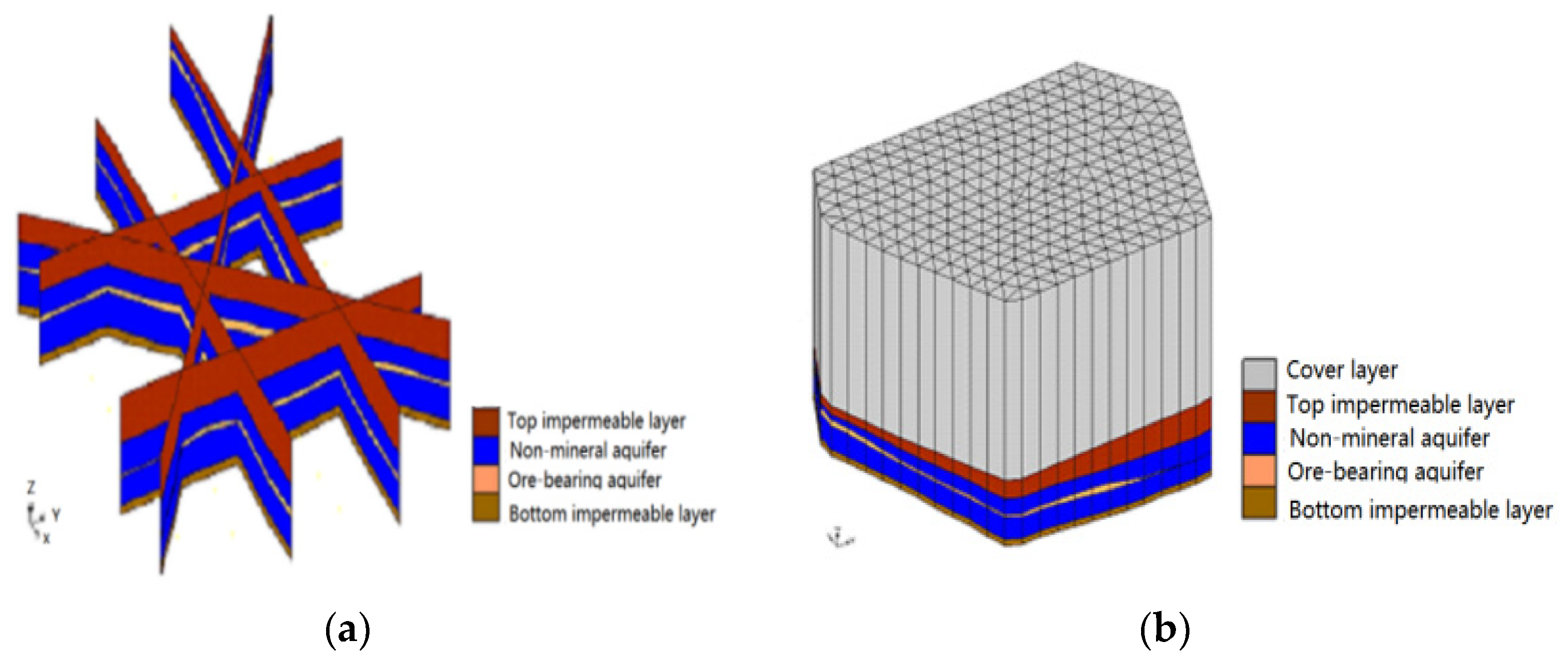
3.1. Geological and Hydrogeological Characteristics of a Uranium Deposit

The study here chooses one of the mining areas of a uranium mine in Northwest China as a research case. The ore type is a leached uranium deposit in the interlayer oxidation zone of the inter-mountain basin. Uranium minerals are mainly pitch uranium ore, containing a small amount of uranium and uranium stone. Uranium ilmenite and uranium-bearing pitch contain uranium minerals, and uranium is absorbed by clay and organic minerals in the cement. Insoluble minerals in the ore account for 93% without harmful ingredients, such as montmorillonite. The ore composition is conducive to in-situ leaching. The upper and lower aquifers of ore body are well developed. The water-bearing rock has good sorting performance, uniform particle composition, and poor degree of cementation. The permeability coefficient of the entire ore-bearing aquifer is between 0.5 and 1.16 m/d. Water inflow of the borehole is 0.06~0.12 L/s·m, groundwater salinity is 0.23~0.69 g/L, and the water temperature is 11~16 °C.

3.2. Model Construction and Reserve Calculation Process

In GMS, the main functional modules for constructing a 3D hydrogeological structure model include borehole, TINs, 2D scatter point and solid modules [36]. The borehole module can be used to convert borehole data into hydrogeological bodies, accurately and truly reflecting the hydrogeological structure. The TINs module can triangulate the spatial area, using interpolation to calculate the specific elevation value on the split node, display the contour map, and realize the spatial distribution of a single interface. Utilizing the 2D scatter point module can manage discrete point data and calculate various contour maps based on the interpolation of discrete data [37,38]. After TINs modeling, the solid module can generate a three-dimensional model of stratum through a series of operations and cut the section at any layer and any position as required to view distribution of stratum on the section. In this study, the scatter point, borehole data, grid, TINs and solid modules are mainly used to build geological models and numerical models. The purpose of establishing the solid model is to master the spatial geometry of the mineral and obtain parameter distribution of ore thickness and uranium grade, so as to lay a foundation for the reserve estimation.

The process of establishing a three-dimensional hydrogeological structure model is as follows: the borehole module converts the borehole data into a hydrogeological body. Each independent borehole is connected to the borehole geological profile through calculation and interpolation (Figure 1a). The solid module converts the borehole profile into a three-dimensional hydrogeological solid model. Figure 1b shows the stratigraphic structure.

Calculation of uranium reserves is as follows: The TINs module constructs an irregular triangular grid and forms a numerical model. First, different grid numbers are selected respectively, and then the grid units of the mining area are subdivided using the 2D scatter point module, and a TIN grid of the geological map is established; successively, the borehole data is input into the TINs module through different interpolation methods, and the contour figures of the reserve parameters are obtained. DATA SET CALCULATOR multiplies the grade and ore thickness of the TIN grid value, and then multiplies it by the density and grid area to obtain a new data set representing the uranium reserves of each grid point. All the data are summed to get the uranium reserves in the mining area. Since the highest value of uranium grade is in range of 6–8 times the overall average value, considering the possible representative significance of ultra-high grade, ultra-high-grade value will not be handled in this study [39].

4. Result and Analysis

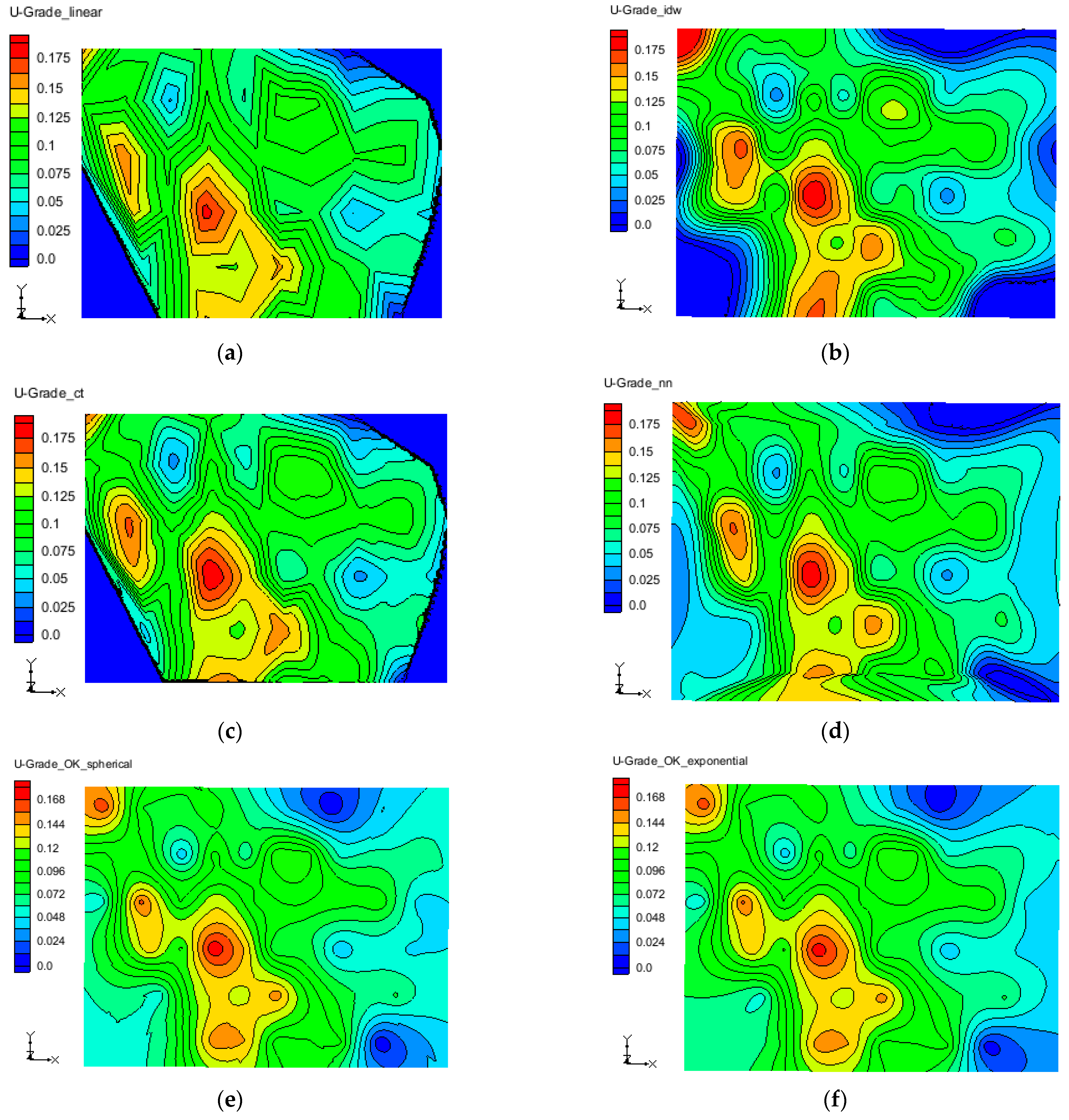
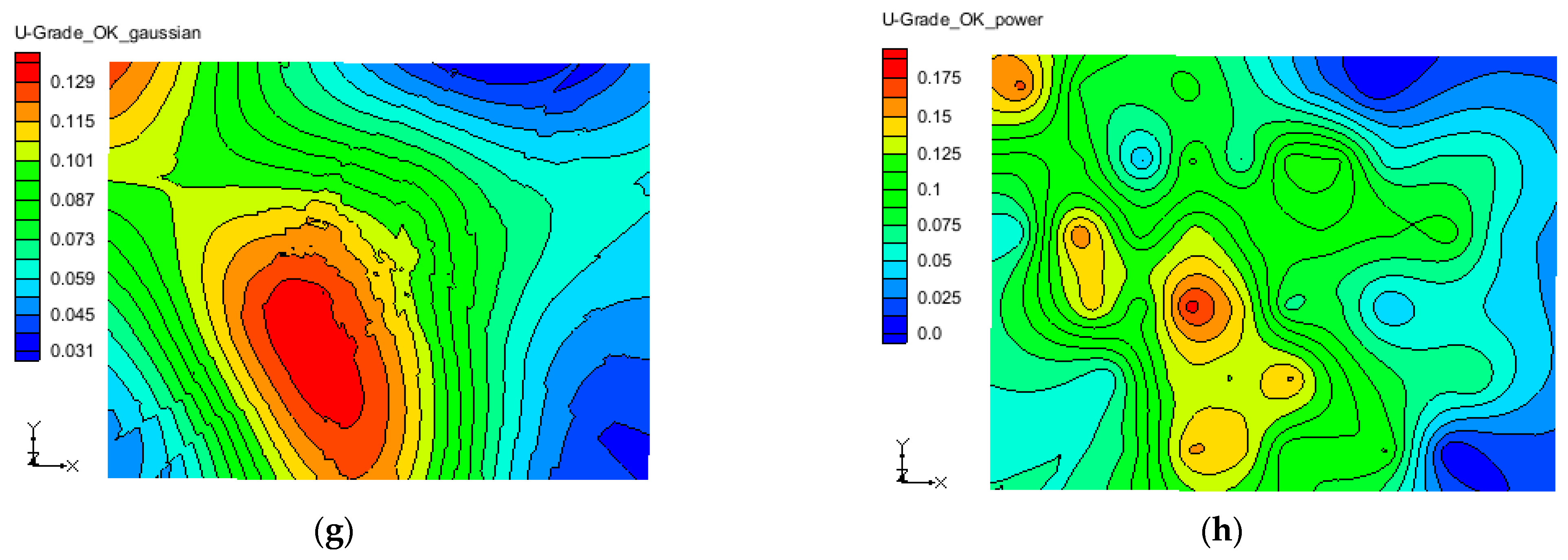
4.1. Analysis of the Distribution of Reserves-Related Parameters

Due to limited sampling points in this study, effects of SK and OK interpolation are very similar when the parameter settings are the same, so the study here mainly uses OK (including spherical, exponential, gaussian and power) and several other interpolation methods (including linear, IDW, CT and NN). The contour map obtained by interpolation calculation can be seen intuitively: (1) The ore thickness is characterized by thicker central and southern areas and thinner surrounding areas. (2) Uranium grades are characterized by high values in the central, southern and west-central locations and low values in other locations. (3) In general, the distribution of uranium content per square meter in the mining area is characterized by high values in the central and southern locations and low values in other locations. The results are consistent with the actual exploration. Figure 2 shows the distribution characteristics of uranium grade under different interpolation methods.

From the effects of several interpolation techniques, the following conclusions can also be drawn: (1) the linear and CT interpolation effects are similar in ore thickness, uranium grade or uranium content per square meter. There is no interpolation in the non set range, but the default value is directly assigned. The interpolation edge of CT method is smoother than that of linear interpolation. (2) For ore thickness and uranium grade in the mining area, the interpolation results of three OK methods (spherical, exponential and power) are similar, but they all estimate the adjacent area outside the boundary just like IDW and NN. Spherical and exponential have a wider range of interpolation in the boundary area. (3) The gaussian is different from the contour maps of other methods. The contour presents a large oval area. The difference in value caused by distance is not as obvious as other interpolation methods. Estimated value of the elliptical area is obviously larger than that of the surrounding area, but its estimated value is less than other interpolation methods.

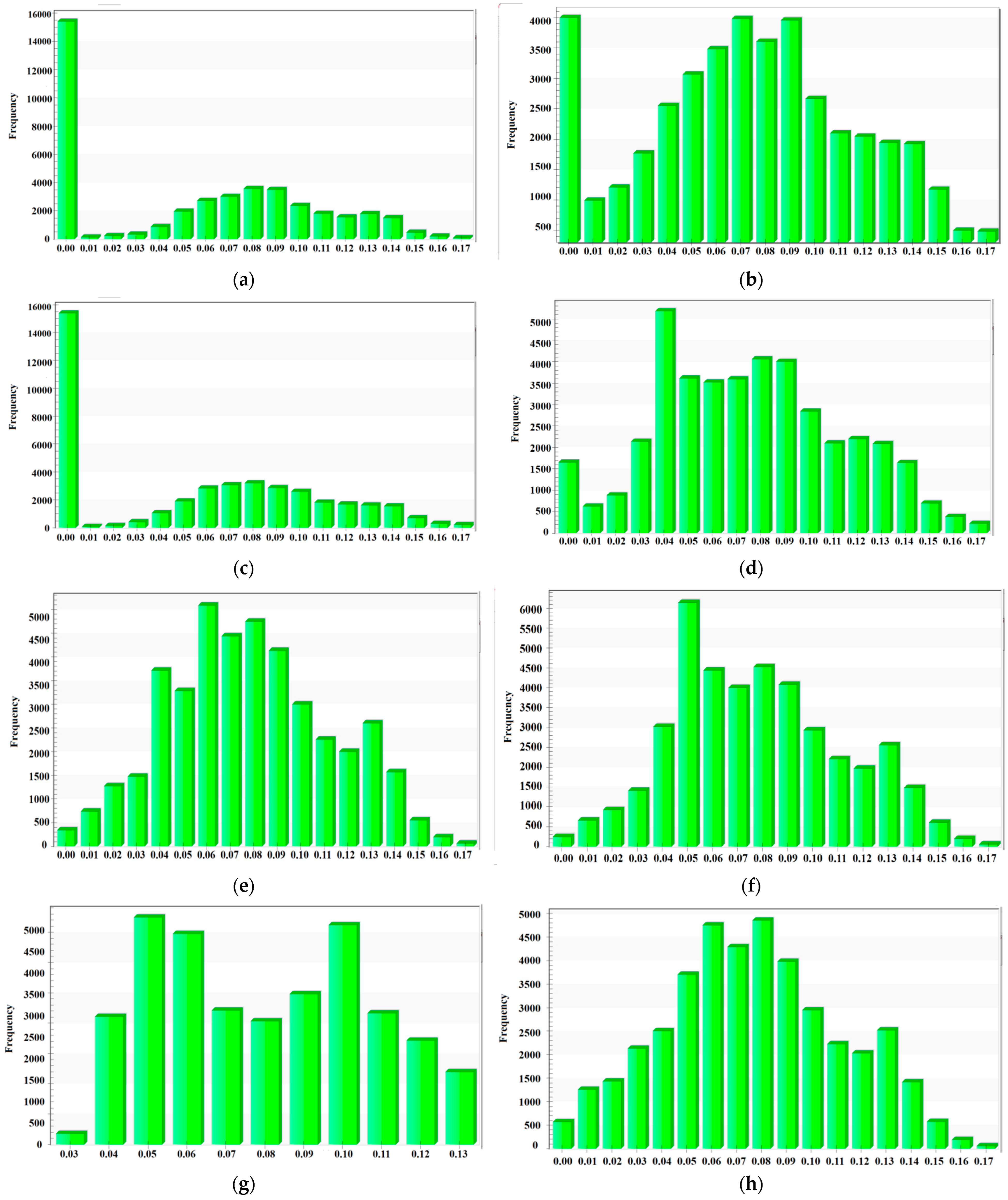
4.2. Analysis of Distribution Frequency of Reserve Parameters

Forty-one thousand four hundred data points are obtained through each interpolation. Figure 3 shows the frequency histogram of uranium grade distribution under different interpolation algorithms. The interval of each histogram is set to 18, except for gaussian. Since the value range after gaussian interpolation is relatively concentrated, the interval is set to 11.The following can be found from the frequency distribution diagram: (1) Using the three interpolation methods (linear, IDW and CT), the reserve parameters (ore thickness, uranium grad, and uranium content per square meters) all have a minimum value of zero. The frequency of zero value is the largest, and the maximum frequency can reach 37%. Using NN interpolation, the minimum value of uranium content per square meters is also zero, and the frequency of occurrence is the largest (16%). The reasons are as follows: firstly, there is a zero value in the sampled borehole data, which means the three reserve parameters of this borehole point are all zero, and the predicted value of this borehole point is also zero after interpolation. Secondly, the value of the area outside the boundary is set to zero and accounts for a large proportion. When calculating reserves, both zero-value grade and zero-value ore thickness have been specially treated. See Section 5.1 for details. (2) The minimum and maximum values of IDW, CT and NN interpolation are the same, and the range value (=maximum-minimum) is higher than other interpolation modes. The range of gaussian interpolation is the smallest. When calculating reserves, the gaussian method is not modified, but the predicted values of the corresponding reserves parameters of each grid point after interpolation are directly used for calculation. (3) As mentioned earlier, the contour maps of linear and CT results are very similar. The frequency map and the interpolation calculation process shows that the frequency and arithmetic average of the three reserve-related parameters are also very close.

Table 1. Comparison of interpolation range and arithmetic mean of several interpolation methods.

Reserve Parameters	Statistical Parameters	Numerical Comparison
Ore thickness	interpolation range	IDW = CT = NN > linear > power > spherical > exponential > gaussian
	arithmetic mean	exponential > spherical > power > NN > IDW > gaussian > linear > CT
Uranium grade	interpolation range	IDW = CT = NN > linear > power > spherical > exponential > gaussian
	arithmetic mean	gaussian > spherical > exponential > power > NN > IDW > CT > linear
Uranium content per square meter	interpolation range	IDW = CT = NN = power > linear > spherical > exponential > gaussian
	arithmetic mean	spherical > exponential > gaussian > power > IDW > NN > CT > linear

lists the comparison of the interpolation range value and the arithmetic mean value between various methods.

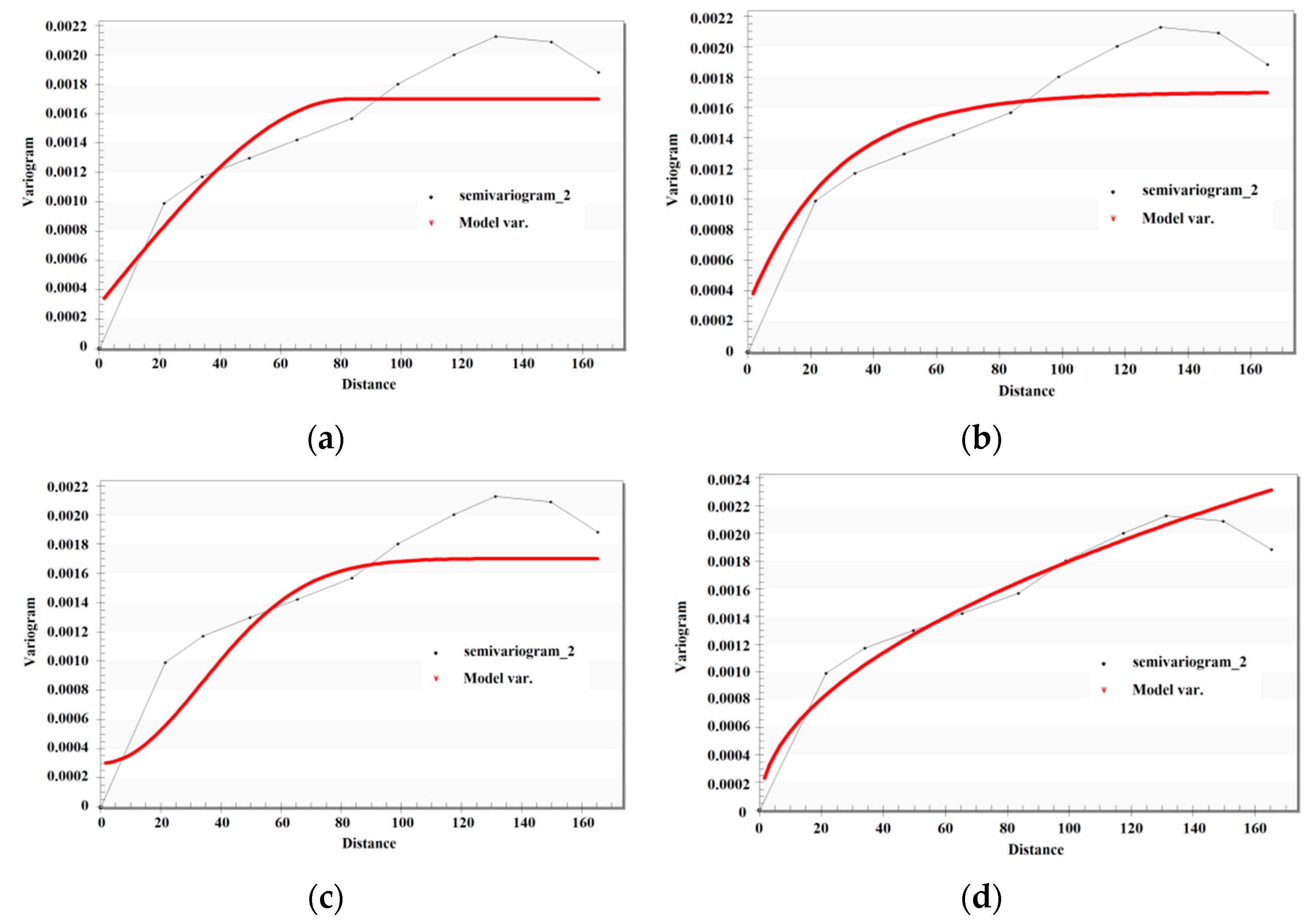
4.3. Semivariogram Analysis

Mainly based on the fact that the estimated parameters meet the second-order stationary hypothesis and the sample size is large enough, kriging interpolation is to obtain the value of the interpolation point through the variogram. The variogram is the core of regionalized variable theory and the basic element of the kriging method. The variogram can not only describe the spatial structural changes of regionalized variables, but also their random changes; that is, the variogram quantifies the spatial correlation of mineralization parameters (e.g., grade, thickness, accumulation, bedrock elevation, etc.) [15]. The semivariogram function is mainly used in GMS to represent the interpolation result, and its value is half of the variogram function. The semivariogram is stated as [40]:

$$\gamma (h)=\frac{1}{2N}{\displaystyle \sum _{i=1}^N[}Z(x_i)-Z(x_i+h){]}^2$$

(6)

where $\gamma (h)$ is semivariogram function value, N is the number of sample pairs, $Z(x_i)$ is the value at point ($x_i$), $Z(x_i+h)$ is the value at point ($x_i+h$) and h is the separation distance in the specified direction between points ($x_i+h$) and ($x_i$).

The study here applied four OK interpolation methods (spherical, exponential, gaussian and power) to construct four different semivariograms. The experimental variogram function curve is a non-smooth sawtooth curve, which requires theoretical curve fitting. The specific parameter settings are shown in

Table 2. Semivariogram parameter setting.

	Parameter	Spherical	Exponential	Gaussian	Power
Ore thickness	Nugget	0.7677	0.7677	0.7677	0.0000
	Contribution	2.9852	2.9852	2.9852	0.5118
	Range	78.5296	78.5296	78.5296	0.4400
Uranium grade	Nugget	0.0003	0.0003	0.0003	0.0000
	Contribution	0.0014	0.0014	0.0014	0.0002
	Range	82.6458	82.6458	82.6458	0.5000
Uranium content per square meter	Nugget	3.3866	3.3866	3.3866	3.3866
	Contribution	20.3198	20.3198	20.3198	0.7380
	Range	49.5924	49.5924	49.5924	0.7400

. Figure 4 shows the experimental variogram (semi variogram) and model variogram of uranium grade. The steps for estimation using kriging are as follows: (1) obtain the variogram model of the deposit, (2) fit the standard model to the variogram and (3) use any available estimation technique to generate block estimates [17].

As can be seen from Table 2: (1) In order to make the experimental variogram and model variogram fit better, spherical, exponential and gaussian methods are the same in nugget, contribution and range settings. Power interpolation only sets the same nugget value as the other three methods in the estimation of uranium content per square meter. (2) It can be seen from the nugget setting value that the setting of uranium content per square meter is the largest and the setting of uranium grade is the smallest, indicating that the uranium grade of regionalization variable changes little in a small range, while the uranium quantity per square meter changes greatly in a small range. (3) As can be seen from the model, variogram curves of the first three methods rise sharply within a certain distance and then gradually slow down until they are close to the level. This shows that the correlation between data in each reserve parameter area first increases and then decreases with the increase of distance, and the inflection point value is the range value. Although the power model variogram fits well with the experimental variogram in uranium grade, the curve always shows an upward trend, but it does not mean that the correlation between the data in area increases with the increase of distance. It can also be concluded that if the distance exceeds the corresponding range value set in Table 2, the regionalization variables (ore thickness, uranium grade and uranium content per square meter) will no longer be relevant. This occurs when spherical, exponential and gaussian interpolation methods are used.

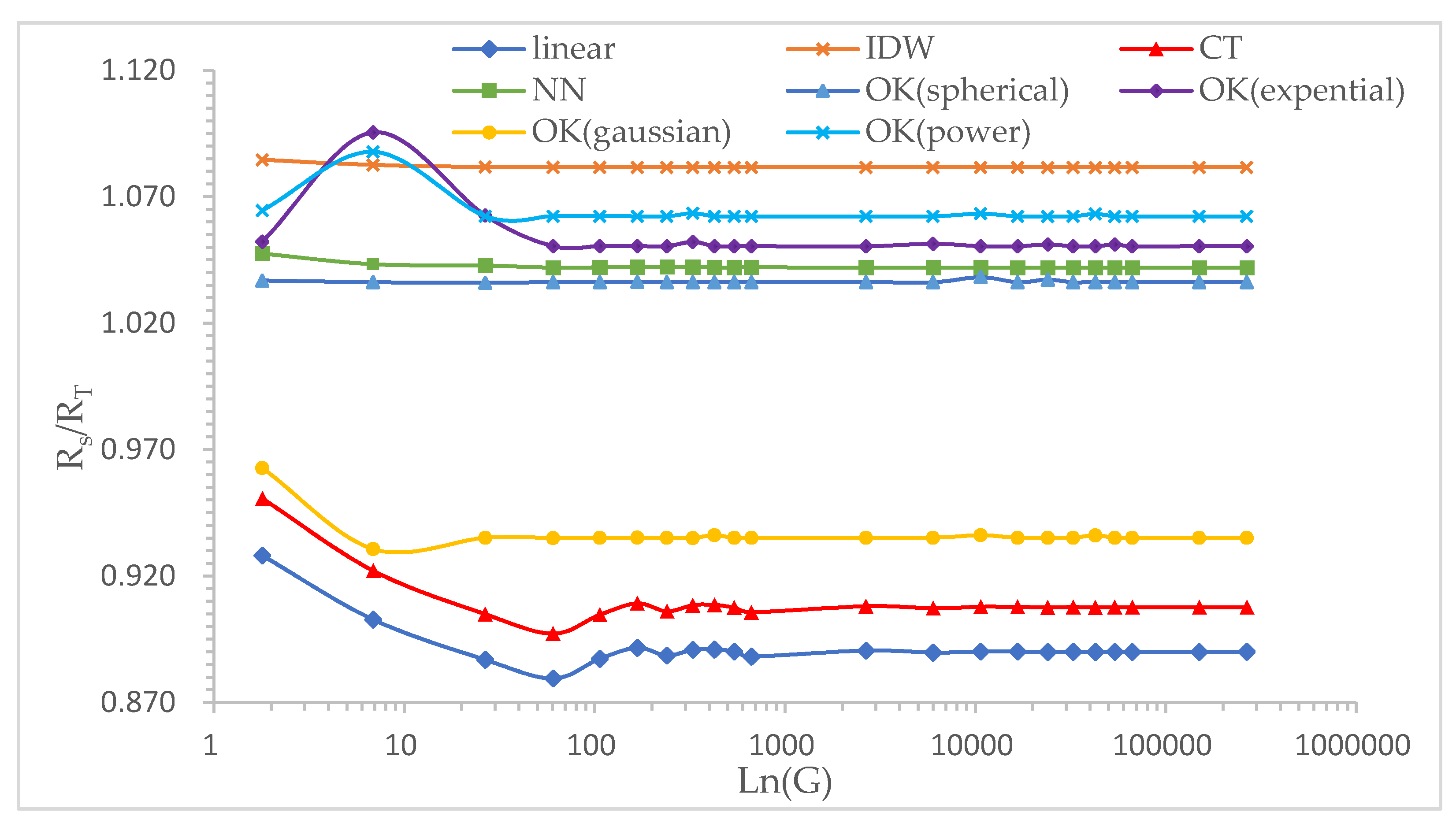
4.4. Cross-Validation and Error Analysis

Cross-validation, still one of the best methods to check interpolation efficiency, is used to test effectiveness of the estimation. One advantage of cross validation is that existing data can be used to evaluate accuracy of spatial distribution without additional sampling [41]. In order to use fitting variogram to achieve the goal, data will be deleted in each step, and its value will be estimated by using different interpolation methods according to other real data in the mining area. Then, the difference between estimated values and actual values is analyzed. The statistics of uranium grade error after cross-validation are obtained according to Formula (7)–(11) [42]. The following conclusions can be drawn from

Table 3. Error analysis after cross-validation of uranium grade.

	Linear	IDW	CT	NN	Spherical	Exponential	Gaussian	Power
MAE	0.0054	0.0037	0.0049	0.0036	0.0022	0.0027	0.0043	0.0031
RMSE	0.0060	0.0049	0.0056	0.0045	0.0032	0.0034	0.0051	0.0042
SD	0.0287	0.0237	0.0301	0.0225	0.0163	0.0166	0.0236	0.0191
COV	0.3743	0.2975	0.3812	0.2797	0.1958	0.2001	0.3084	0.2341

: (1) The MAE and RMSE of the methods all tend to be zero, which proves that these interpolation effects are good. (2) In general, the closer the RMSE is to zero, the closer the estimated value is to the actual value. It can be inferred from the RMSE that the order of interpolation effect from superior to inferior is: spherical > exponential > power > NN > IDW > gaussian > CT > linear. (3) The coefficient of variation (COV) value of the five methods (spherical, exponential, power, NN and IDW) is within 30%, while the COV value of the other three interpolation methods (gaussian, CT and linear) is controlled within 39%. (4) It can also be concluded from cross-validation that the estimated value of gaussian is generally low compared to the other three OK methods mentioned in the current study.

$$\mathrm{Standard} \mathrm{deviation} (\mathrm{SD}): \sigma =\sqrt{\frac{1}{n}{\displaystyle \sum _{i=1}^n{[Z(x_i)-\overline{Z}(x_i)]}^2}} \mathrm{or} \sigma =\sqrt{\frac{1}{n}{\displaystyle \sum _{i=1}^n{[\widehat{Z}(x_i)-\overline{\widehat{Z}}(x_i)]}^2}}$$

(7)

$$\mathrm{Coefficient} \mathrm{of} \mathrm{variation} (\mathrm{COV}): c_v=\frac{\sigma }{\overline{Z}(x_i)}\times 100\% \mathrm{or} c_v=\frac{\sigma }{\overline{\widehat{Z}}(x_i)}\times 100\%$$

(8)

$$\mathrm{Root} \mathrm{mean} \mathrm{squared} \mathrm{error} (\mathrm{RMSE}): \mathrm{RMSE}=\sqrt{\frac{1}{n}{\displaystyle \sum _{i=1}^n{[Z(x_i)-\widehat{Z}(x_i)]}^2}}$$

(9)

$$\mathrm{Mean} \mathrm{absolute} \mathrm{error} (\mathrm{MAE}): \mathrm{MAE}=\frac{1}{n}{\displaystyle \sum _{i=1}^n|Z(x_i)-\widehat{Z}(x_i)|}$$

(10)

$$\mathrm{Mean}: \overline{Z}(x_i)=\frac{1}{n}{\displaystyle \sum _{i=1}^{n}Z(x_i}) \mathrm{or} \overline{\widehat{Z}}(x_i)=\frac{1}{n}{\displaystyle \sum _{i=1}^n\widehat{Z}(x_i})$$

(11)

where $Z(x_i)$ is the observed (known) value, $\widehat{Z}(x_i)$ is the predicted value and n is the number of values in the dataset.

5. Comparison of Traditional Calculation and Interpolation Estimation Results of Uranium Reserves

5.1. Traditional Calculation Formulas and Interpolation Estimation Formulas

Currently, reserve prediction of sandstone uranium is mainly based on quantitative gamma logging data of exploration boreholes. The main calculation method is to use the weighted average of all drilling grades in the unit as the average ore grade in the block, and the thickness is the weighted average of all drilling thicknesses. Finally, the uranium metal reserves in the block are estimated in combination with ore density and other data [10], as follows:

$${\mathrm{R}}_{\mathrm{T}}=\mathrm{U}\times \mathrm{A}$$

(12)

$$\mathrm{Or} {\mathrm{R}}_{\mathrm{T}}=\mathrm{c}\times \mathrm{m}\times \mathrm{d}\times \mathrm{A}$$

(13)

where ${\mathrm{R}}_{\mathrm{T}}$ is uranium reserves (kg), subscript T represents the traditional calculated value, A is the total area of uranium distribution (m²), U is uranium content per square meter (kg/m²), c is the average grade (%), m is ore thickness (m) and d is ore density (kg/m³).

The calculation formula of uranium content per square meter is similar to both single project and block section, as shown below [2]:

$$\mathrm{U}=\mathrm{c}\times \mathrm{m}\times \mathrm{d}$$

(14)

Accuracy of the calculation results obtained from Formula (12) or (13) depends on the borehole data. The more boreholes, the more detailed the data, and the more accurate the calculation results. However, from an economic viewpoint, numbers of boreholes in each mining area are not large, so there is a gap between the calculated results and the actual reserves.

In order to reduce calculation error caused by limited borehole data, the tool of interpolation and data calculation of GMS software is used to calculate uranium reserves. The formula is as follows:

$${\mathrm{R}}_{\mathrm{s}}={\displaystyle \sum _{\mathrm{i}=1}^{\mathrm{n}}{\mathrm{c}}_{\mathrm{i}}\times {\mathrm{m}}_{\mathrm{i}}\times {\mathrm{d}}_{\mathrm{i}}\times {\mathrm{A}}_{\mathrm{i}}}$$

(15)

$$\mathrm{Or} {\mathrm{R}}_{\mathrm{s}}={\displaystyle \sum _{\mathrm{i}=1}^{\mathrm{n}}{\mathrm{U}}_{\mathrm{i}}\times {\mathrm{A}}_{\mathrm{i}}}$$

(16)

where ${\mathrm{R}}_{\mathrm{s}}$ is the total reserves of uranium in the mining area (kg), the subscript S represents the estimated value, ${\mathrm{c}}_{\mathrm{i}}$ is the uranium grade of the i grid cell (%), ${\mathrm{m}}_{\mathrm{i}}$ is the ore thickness of the i grid cell (m), ${\mathrm{d}}_{\mathrm{i}}$ is the ore density of the i grid cell (kg/m³), ${\mathrm{A}}_{\mathrm{i}}$ is the area of the i grid cell (m²) and ${\mathrm{U}}_{\mathrm{i}}$ is the uranium content per square meter of the i grid cell (kg/m²).

Since the depth is less than 500 m, when uranium grade, ore thickness and uranium content per square meter are zero, and the parameter values are set as follows: (1) In the boundary area, the uranium grade is set to 0.01%. The uranium content per square meter is set to 1 kg/m². (2) In non-boundary areas, the uranium grade is estimated to be 0.005%. The uranium content per square meter is 0.5 kg/m² [12]. The ore thickness is equal to the minimum value of the interpolation near the point.

5.2. Comparative Analysis of Uranium Reserve Estimation Results

The parameter G is set as the ratio of the number of grids in the mining area model to the actual number of geological boreholes in the mining area. R_S/R_T and parameter G logarithmic function ln(G) curves are constructed as shown in Figure 5, where, R_T and R_S represent traditionally calculated uranium reserves and estimated uranium reserves, respectively.

Figure 5 shows that linear interpolation and CT interpolation have similar function changes, which can be divided into three stages (1) when ln(G) is within 60, the curves decrease sharply with the increase of the number of grids; (2) when ln(G) is within the range of 60 to 664, the curves oscillate slightly with the increase of the grid number; (3) when ln(G) is larger than 664, the curves basically remain unchanged with the increase of ln (G). The variation curves obtained by NN and IDW are similar. The curves decrease slightly within 7 with the increase of ln(G) and remain basically unchanged when larger than 7. The spherical interpolation curve is basically a straight line, which means that the ratio of grid setting value to the number of boreholes has little effect on reserve related parameters of spherical calculation. The exponential curve, power curve and gaussian curve are also very similar: when ln(G) is above 7, the relative errors all show an upward trend; when ln(G) is between 7 and 27, the relative errors all show a downward trend; when ln(G) is equal to 7, the relative error $\mathsf{\delta }$ (Formula (17)) of exponential is larger than that of power and gaussian; however, when ln(G) is equal to 60, the three curves begin to stabilize. The absolute value of the relative error is compared as: ${\mathsf{\delta }}_{\mathrm{gaussian}}$ > ${\mathsf{\delta }}_{\mathrm{exponential}}$ > ${\mathsf{\delta }}_{\mathrm{poewr}}$. As the number of boreholes increases, the estimated values of the three methods will not change much.

The estimation of uranium reserves is evaluated in combination with Figure 5 and relative error. The simulation results of Rs showed that estimation values of the five methods (IDW, power, exponential, NN and spherical) are all larger than the traditional calculation values, while the interpolation results of the other three methods (gaussian, CT and linear) are less than the traditional calculation values. As shown in

Table 4. Relative error of uranium reserves.

	Linear	IDW	NN	CT
Relative error	−10.98%	+8.16%	+4.20%	−9.22%
	Spherical	Exponential	Gaussian	Power
Relative error	+3.62%	+5.13%	−6.49%	+6.32%

, the relative errors of several interpolation methods are all controlled within ±10.98%. The relative error here is the approximate value when the curve in Figure 5 tends to be stable. The relative error of spherical interpolation result is the smallest and closest to actual calculated value. The relative error of other OK methods is also relatively small, which further verifies the advantage of kriging. In this case, NN is a traditional interpolation method whose simulation effect is second only to spherical, closer to the traditional calculation value than IDW. The likely reason is that in the interpolation process the frequency of low value (= 0.005%) in uranium grade is too high in linear, IDW and CT when excluding the zero value outside the boundary, which results in increased calculation error.

$$\mathsf{\delta }=\frac{{\mathrm{R}}_{\mathrm{S}}-{\mathrm{R}}_{\mathrm{T}}}{{\mathrm{R}}_{\mathrm{T}}}\times 100\%$$

(17)

The above rule showed that the design of grids number has a certain relationship with the actual number of boreholes. Different interpolation methods have certain requirements for the design of grid numbers. When value in the appropriate range is reached, the simulation results will reach a higher accuracy. If the number of grids increases continuously, the effect on the interpolation results will be very small, while computer running time and storage space will increase substantially. However, the spherical method does not seem to be affected by the ratio of the number of grids to the number of boreholes. Appropriate grid design still needs to be considered to avoid large errors in the interpolation estimation of other reserve parameters. In this case, the measured data values are compared to optimize the number of grids.

6. Conclusions and Future Works

In the process of uranium exploration and development, the distribution of mineral resources and reserve estimation are of great significance to the economic evaluation of uranium deposits. Through the analysis of sandstone uranium deposit data in the Xinjiang Region, the following conclusions are drawn:

(1)

Due to complexity of the underground environment in which the sandstone uranium mine is located and the particularity of the leaching method, the study here chooses GMS to combine traditional geological research with computer applications, and the exploration data is quickly converted into a visual 3D model through different interpolation methods, saving calculation time and improving work efficiency. It does not require a large number of auxiliary drawings like the traditional calculation methods. Even if the design conditions change, as long as the corresponding parameters and commands are altered, a new geological model can be built, and a dynamically changing uranium value can be obtained in the subsequent leaching process.

(2)

The differences of various interpolation methods are analyzed quantitatively by comparing and analyzing the distribution characteristic map, frequency histogram and statistical characteristic value. These interpolation methods are linear, IDW, CT, NN, spherical, exponential, gaussian and power. The last four models are based on the kriging principle. Both the regional prediction of reserve parameters and estimation of reserve value verified the advantages of the kriging method in interpolation calculation, especially the spherical model, and the relative error of reserves is +3.62%.

(3)

Using software to analyze geological data, design of the grid should refer to number of boreholes, and the ratio of the two should be set in an appropriate range (different interpolation methods use different ratios) to improve accuracy and save calculation time and storage space.

(4)

Although object of the study is proven (pre-feasibility study) economic basic reserves (121b), the calculation method is also applicable to resource/reserve estimation of other sandstone uranium mines.

(5)

Due to limitation of exploration data in the study, uranium distribution of the same borehole is assumed to be homogeneous, and the mineral density is equal to the mean value. The future research can be extended to the field of three-dimensional heterogeneity, so the established model will be more in line with the realistic and complex geological conditions, which will reduce estimation errors.

References

1. Afeni, T.B.; Akeju, V.O.; Aladejare, A.E. A comparative study of geometric and geostatistical methods for qualitative reserve estimation of limestone deposit. Geosci. Front. 2020, 12, 243–253. [Google Scholar] [CrossRef]
2. Zhang, J.D.; Wang, C.; Yu, S.Q.; Chen, S.D.; Guo, S.M.; Ding, M.S.; Tan, H.Z. Exploration Specifications on In-Situ Leaching Sandstone Type Uranium Deposits; Standard No. EJ/T 1157-2002; National Defense Science, Technology and Industry Commission: Beijing, China, 2002. [Google Scholar]
3. Abzalov, M.Z.; Drobov, S.R.; Gorbatenko, O.; Vershkov, A.F.; Bertoli, O.; Renard, D.; Beucher, H. Resource estimation of In Situ leach uranium projects. Appl. Earth Sci. 2014, 123, 71–85. [Google Scholar] [CrossRef] [Green Version]
4. Turcotte, D.L. A fractal approach to the relationship between ore grade and tonnage. Econ. Geol. 1986, 81, 152–1532. [Google Scholar] [CrossRef]
5. Skvortsova, T.; Beucher, H.; Armstrong, M.; Forkes, J.; Thwaites, A.; Turner, R. Simulating the Geometry of a Granite-Hosted Uranium Orebody. In Geostatistics Rio 2000, Proceedings of the 31st International Geological Congress, Rio de Janeiro, Brazil, 6–17 August 2000; Quantitative Geology and Geostatistics; Armstrong, M., Bettini, C., Champigny, N., Galli, A., Remacre, A., Eds.; Kluwer Academic Publishers: Dordrecht, The Netherlands, 2002. [Google Scholar] [CrossRef]
6. Petit, G.; Boissezon, H.D.; Langlais, V.; Rumbach, G.; Khairuldin, A.; Oppeneau, T.; Fiet, N. Application of stochastic simulations and quantifying uncertainties in the drilling of roll front uranium deposits. In Geostatistics Oslo 2012; Springer: Dordrecht, The Netherlands, 2012; pp. 321–332. [Google Scholar] [CrossRef]
7. Yang, L.R. Research on 3D Modeling of Complex Orebody Structure and Reserve Calculation with Uranium Deposits as an Example. Ph.D. Thesis, Chengdu University of Technology, Chengdu, China, 2013. [Google Scholar]
8. Qi, J.Q.; Zhang, J.X.; Liu, Y. The Application of Digital Geological Survey System in Resource Estimation for Uranium Deposit and 3D Orebody Modeling. Uranium Geol. 2019, 35, 373–377. [Google Scholar] [CrossRef]
9. Bai, Y.; Zhu, P.F.; Zhu, J.; Kong, W.H.; Li, X.C.; Cao, K.; Sun, L.; Liu, L.Y. Application of geo-statistics in calculation of a uranium deposit. In Earth Geological Energy Mining and Landform Protection, Proceedings of the 2020 2nd International Conference on Geoscience and Environmental Chemistry (ICGEC 2020), Tianjin, China, 9–11 October 2020; E3S Web of Conferences; EDP Sciences: Les Ulis, France, 2020; Volume 206, pp. 1–7. [Google Scholar] [CrossRef]
10. Li, Z.K.; Yang, R.; Hu, B.S.; Du, Z.M.; Zhao, L.X. Reserve prediction method of sandstone uranium reservoir based on data of natural gamma logging while drilling. At. Energy Sci. Technol. 2021, 55 (Suppl. S2), 373–379. [Google Scholar] [CrossRef]
11. Cui, T.; Yang, Y. An advanced uranium ore grade estimation method based on photofission driven by an e-LINAC. Nucl. Instrum. Methods Phys. Res. Sect. A Accel. Spectrom. Detect. Assoc. Equip. 2021, 1014, 165710. [Google Scholar] [CrossRef]
12. Zhang, J.D.; Yu, H.X.; Yu, S.Q.; Liu, X.Y. Guidebook on Resources/Reserves Estimation for In-Situ Leaching Sandstone Type Uranium Deposits; Standard No. EJ/T 1214-2016; State Administration of Science, Technology and Industry for National Defense: Beijing, China, 2016. [Google Scholar]
13. Liang, H.J. China’s Mineral Resources/Reserves Estimation Method. Master’s Thesis, China University of Geosciences, Beijing, China, 2018. [Google Scholar]
14. Lan, Y.R.; Tang, Y. What is the SD method. Geol. Rev. 2000, 46 (Suppl. S1), 329–336. [Google Scholar]
15. Gandhi, S.M.; Sarkar, B.C. Chapter 12—Geostatistical resource/reserve Estimation. In Essentials of Mineral Exploration and Evaluation; Elsevier Inc.: Amsterdam, The Netherlands, 2016; pp. 289–308. [Google Scholar] [CrossRef]
16. Haldar, S.K. Chapter 9—Statistical and Geostatistical Applications in Geology. In Mineral Exploration, 2nd ed.; Elsevier Inc.: Amsterdam, The Netherlands, 2018; pp. 167–194. [Google Scholar] [CrossRef]
17. Jalloh, A.B.; Kyuro, S.; Jalloh, Y.; Barrie, A.K. Integrating artificial neural networks and geostatistics for optimum 3D geological block modeling in mineral reserve estimation: A case study. Int. J. Min. Sci. Technol. 2016, 26, 581–585. [Google Scholar] [CrossRef]
18. Kreuzer, O.P.; Markwitz, V.; Porwal, A.K.; McCuaig, T.C. A continent-wide study of Australia’s uranium potential. Ore Geol. Rev. 2010, 38, 334–366. [Google Scholar] [CrossRef]
19. Joly, A.; Porwal, A.; McCuaig, T.C.; Chudasama, B.; Dentith, M.C.; Aitken, A.R.A. Mineral systems approach applied to GIS-based 2D-prospectivity modelling of geological regions: Insights from Western Australia. Ore Geol. Rev. 2015, 71, 673–702. [Google Scholar] [CrossRef]
20. Zhou, D.; Jiang, Y.B. The building and application of three-dimensional geological model with the 3DMine software in the third belt of Zoujiashan uranium deposit. J. Geol. 2017, 41, 91–96. [Google Scholar] [CrossRef]
21. Ciputra, R.; Suharji, S.; Kamajati, D.; Syaeful, H. Application of geostatistics to complete uranium resources estimation of Rabau Hulu Sector, Kalan, West Kalimantan. In Land, Water, and Natural Resources, Proceedings of the 1st Geosciences and Environmental Sciences Symposium (ICST 2020), Yogyakarta, Indonesia, 7–8 September 2020; E3S Web of Conferences; EDP Sciences: Les Ulis, France, 2020; pp. 1–7. [Google Scholar] [CrossRef]
22. Wang, H.M.; Kong, F.H.; Song, Q.L. Micromine software application on 3D modeling and resource estimate in the ferrum desposit: An example from Cameroon Lobi iron deposit. North China Geol. 2014, 2, 144–148. [Google Scholar] [CrossRef]
23. Taghvaeenezhad, M.; Shayestehfar, M.; Moarefvand, P.; Rezaei, A. Quantifying the criteria for classification of mineral resources and reserves through the estimation of block model uncertainty using geostatistical methods: A case study of khoshoumi uranium deposit in Yazd, Iran. Geosyst. Eng. 2020, 23, 216–225. [Google Scholar] [CrossRef]
24. Hou, M.Q.; Wu, Z.C.; Guo, F.S.; Luo, J.Q.; Wang, F. Establishment of a three-dimensional geological model of the Zoujiashan-Julong’an area in Le’an of Jiangxi Province. J. Geol. 2016, 40, 118–124. [Google Scholar] [CrossRef]
25. GMS: What Is GMS. Available online: https://www.xmswiki.com/wiki/GMS:What_Is_GMS (accessed on 17 July 2021).
26. GMS: Linear. Available online: https://www.xmswiki.com/wiki/GMS:Linear (accessed on 17 July 2021).
27. Bartier, P.M.; Keller, C.P. Multivariate interpolation to incorporate thematic surface data using inverse distance weighting (IDW). Comput. Geosci. 1996, 22, 795–799. [Google Scholar] [CrossRef]
28. GMS: Inverse Distance Weighted. Available online: https://www.xmswiki.com/wiki/GMS:Inverse_Distance_Weighted (accessed on 17 July 2021).
29. Sibson, R. A brief description of natural neighbor interpolation. In Interpreting Multivariate Data; Wiley: Hoboken, NJ, USA, 1981; pp. 21–36. [Google Scholar]
30. Beutel, A.; Mølhave, T.; Agarwal, P.K. Natural neighbor interpolation based grid DEM construction using a GPU. In Proceedings of the 18th SIGSPATIAL International Conference on Advances in Geographic Information Systems—GIS ‘10, San Jose, CA, USA, 2–5 November 2010; Agrawal, D., Zhang, P., Abbadi, A.E., Mokbel, M., Eds.; Association for Computing Machinery: New York, NY, USA, 2010. [Google Scholar] [CrossRef] [Green Version]
31. Clough, R.W.; Tocher, J.L. Finite element stiffness matrices for analysis of plate bending. In Proceedings of the Conference on Matrix Methods in Structural MechFinite Element Stiffness Matrices for Analysis of Plate Bendinganics, Fairborn, OH, USA, October 1965. [Google Scholar]
32. Lancaster, P.; Šalkauskas, K. Curve and Surface Fitting: An Introduction; Academic Press: London, UK, 1986; Volume 31, pp. 155–157. [Google Scholar] [CrossRef]
33. Oqielat, M.N. Surface fitting methods for modelling leaf surface from scanned data. J. King Saud Univ.-Sci. 2019, 31, 215–221. [Google Scholar] [CrossRef]
34. Ali Akbar, D. Reserve estimation of central part of Choghart north anomaly iron ore deposit through ordinary kriging method. Int. J. Min. Sci. Technol. 2012, 22, 573–577. [Google Scholar] [CrossRef]
35. Oliver, M.A.; Webster, R. Kriging: A method of interpolation for geographical information systems. Int. J. Geogr. Inf. Syst. 1990, 4, 313–332. [Google Scholar] [CrossRef]
36. Shao, A.J.; Chen, J.H.; Huang, Y. 3D Visual Geology-Modeling in Wannian Mine of Fengfeng Coalfield. Adv. Mater. Res. 2013, 671–674, 2072–2075. [Google Scholar] [CrossRef]
37. Zhang, L.; Dong, D.; Zhang, F.; Xu, Z. A novel three-dimensional mine area hydrogeological model based on groundwater modeling systems. J. Coast. Res. 2020, 105 (Suppl. S1), 141–146. [Google Scholar] [CrossRef]
38. Jabbari, E.; Fathi, M.; Moradi, M. Modeling groundwater quality and quantity to manage water resources in the Arak aquifer, Iran. Arab. J. Geosci. 2020, 13, 663. [Google Scholar] [CrossRef]
39. Gao, L.M.; Li, J.; Ju, J.H.; Bo, Z.P.; Wang, F.; Yang, Q.; Chen, H.; Wang, H.Y.; Wan, H.; Song, F.; et al. General Requirements for Mineral Exploration; Standard No. GB/T13908-2020; China Quality and Standards Publishing & Media Co., Ltd.: Beijing, China, 2020. [Google Scholar]
40. Maroufpoor, S.; Bozorg-Haddad, O.; Chu, X. Chapter 9—Geostatistics: Principles and methods. In Handbook of Probabilistic Models; Pijush, S., Dieu, T.B., Subrata, C., Ravinesh, C.D., Eds.; Butterworth-Heinemann: Kidlington, UK, 2020; pp. 229–242. [Google Scholar] [CrossRef]
41. Wadoux, A.M.J.-C.; Heuvelink, G.B.M.; De Bruin, S.; Brus, D.J. Spatial cross-validation is not the right way to evaluate map accuracy. Ecol. Model. 2021, 457, 109692. [Google Scholar] [CrossRef]
42. Robinson, T.P.; Metternicht, G. Testing the performance of spatial interpolation techniques for mapping soil properties. Comput. Electron. Agric. 2006, 50, 97–108. [Google Scholar] [CrossRef]
Figure 1. Mining area model constructed by GMS. (a) Three-dimensional geological profile of the mining area; (b) Three-dimensional stratigraphic map of the mining area.
Processes 10 00067 g001
Figure 2. Distribution characteristics of uranium grade under different interpolation methods. (a) Linear; (b) IDW; (c) CT; (d) NN; (e) OK(spherical); (f) OK(exponential); (g) OK(gaussian); (h) OK(power).
Processes 10 00067 g002aProcesses 10 00067 g002b
Figure 3. Frequency histogram of uranium grade distribution under different interpolation algorithms. (a) Linear(interval = 18); (b) IDW(interval = 18); (c) CT(interval = 18); (d) NN(interval = 18); (e) OK(spherical)(interval = 18); (f) OK(exponential)(interval = 18); (g) OK(gaussian)(interval = 11); (h) OK(power)(interval = 18).
Processes 10 00067 g003
Figure 4. Experimental variogram and model variogram of uranium grade. (a) OK(spherical); (b) OK(exponential); (c) OK(gaussian); (d) OK(power).
Processes 10 00067 g004
Figure 5. The relationship curve between RS/RT and Ln(G).
Processes 10 00067 g005