Development of a Contactless Conductivity Sensor in Flowing Micro Systems for Cerium Nitrate

Abstract

Impedance spectroscopy has a high potential to detect chemical reactions in flowing systems. In this work, the approach using impedance spectroscopy as a possible analytical tool for a continuous hydrothermal syntheses (CHTS) is presented. With the CHTS-process, it is possible to produce metalloxide nanoparticles with a close particle size distribution and specific surface properties. For this, it is necessary to evaluate the electrode geometry, frequency and other factors influencing the impedance with respect to concentration measurements. In case of frequency-sweep measurements possible electrode geometries for ${\mathrm{C}}^4\mathrm{D}$-Sensors (capacitively coupled contactless conductivity detection) are evaluated. Then distinguishability and reproducibility are tested applying titration measurements to show the ability for concentration detection in constant flow systems. The possibility to measure concentration changes in flowing systems in a reproducible and fast manner as well as with high distinguishability for the test solution cerium nitrate will be presented. Furthermore, the major influencing-factors like electrode geometry, frequency etc. could be determined. It has been shown that with increasing electrode spacing and electrode width, the distinguishability of the concentrations increases and shifts them to lower frequencies.

1. Introduction

Over time, the focus of chemical reactions has shifted from analysis of the final product to in situ analysis in the process. Therefore, in recent decades, more and more measurement methods have been developed that can characterize different components in flowing systems. An extremely powerful method for this are high-frequency impedance measurements. The first investigation of high-frequency impedance measurements were conducted in the 1950s [1,2]. With proceeding technical developments, the measurements became more simple, cheaper and flexible. Therefore, in the 1990s, a high interest developed into this measurements and a rapid growing in research began, continuing up to now [3,4]. Since then, high-frequency impedance measurements mostly called “capacitively coupled contactless conductivity detection”, abbreviated as ${\mathrm{C}}^4\mathrm{D}$ have been applied. Most of the published research is related to the detection in capillary zone electrophoresis (CE) [5,6,7,8]. The present work deals with typical geometric arrangements of the detection electrodes. There are some other works, which investigated the influence of the electrode width and distance already [9,10]. New in this work is a high wall thickness of the isolating tube, which is necessary for the application at the CHTS—plant (Continuous Hydrothermal Synthesis) in the laboratory and the use of cerium nitrate as electrolyte. The CHTS—process deals with near- or supercritical water [11]. Furthermore, this paper evaluates the influences of cell geometry, frequency, tube wall thickness and the concentration of ${\mathrm{Ce}(\mathrm{NO}}_3{)}_3$ on the impedance. Therefore, the aim of this work is to increase the distinguishability of cerium nitrate concentration by means of impedance by optimizing the aforementioned influencing factors. Finally, this work shows a possibility for an indirect concentration measurement method in flowing systems. This concentration measurement makes it possible to determine the residual concentration after the reaction in order to be able to estimate the conversion of the reaction.

2. Basic Theoretical Considerations

Figure 1a represents a simplified electric equivalent circuit and Figure 1b a schematic picture of the used impedance cell. The measurement principle is based on an applied alternating voltage at high frequencies at the working electrode. At the counter electrode the interaction of the alternating electrical field with the electrolyte is monitored in the form of an impedance signal. At this test setup, the two electrodes were separated from the electrolyte by a thick alumina tube, which is like a dielectric layer and represents two capacitors. In Figure 1a the two capacitors are combined to one Constant Phase Element $\left({CPE}_{cpl}\right)$ according to Kirchhoff’s law. The capacitance of this Constant Phase Element is depended predominantly on the permittivity and thickness of the dielectric layer. Due to the less than ideal smooth surface of the tubes, a CPE is used for these capacities. The electrical behavior of the electrolyte are described by a parallel combination of the capacity and the resistance of the electrolyte. The capacity of the electrolyte is not ideal, therefore a constant phase element ($CP{E}_m$) instead of a ideal capacitor is used. Another part of the electrical energy is a stray (parasitic) capacitance $C_x$, which is represented in the equivalent circuit with the capacitor $C_x$, parallel to the main path. To avoid the effect of stray capacitance, there is often a shielding foil between the electrodes [12,13].

The analytical equation for the impedance of the equivalent circuit contained all impedances of each part. In general, the impedance (Z) is given by equation:

$$Z=R+iX$$

(1)

where the resistance R represents the real part and it is a function of the electrical conductivity of the electrolyte and the cell geometry. There are several factors influencing the imaginary part $\left(X\right)$, which occurs, for example, in capacitors or inductors. These are on the one hand the geometry of the electrodes and on the other hand the relative permittivities of the electrolyte and likewise of the dielectric layer. Furthermore, the imaginary part depends on the frequency of the alternating input signal. Here, i is the imaginary unit. In fact, there are many influencing factors on the behavior of the impedance cell and all of them affects each other. Therefore, it is necessary to consider all these parameters combined when investigating the behavior of an impedance cell. It is also important to determine the best cell geometry for the contactless conductivity detection. In this case, the resistance term ($R_m$) has to predominate, otherwise if the capacitance dominate, it is a dielectrometrical measurement [14]. The impedance of the electric equivalent circuit in Figure 1a can be given, considering Kirchhoff’s law as:

$$Z={\left[\frac{1}{Z\left(CP{E}_{cpl}\right)+{\left[\frac{1}{Z\left(CP{E}_m\right)}+\frac{1}{Z\left(R_m\right)}\right]}^{-1}}+\frac{1}{Z\left(C_x\right)}\right]}^{-1}$$

(2)

$CP{E}_{cpl}$ represents the two coupled capacitors of the electrodes (Figure 1b). $CP{E}_m$ is the capacitive impedance of the electrolyte and $R_m$ is the resistance of the electrolyte. $C_x$ is the parasitic capacitance. Due to these definitions and the definitions of each impedance equation, Equation (2) transforms to Equation (3), with $Q_1$, ${\alpha }_1$ as parameters of $CP{E}_m$ and $Q_2$ and ${\alpha }_2$ as parameters of $CP{E}_{cpl}$:

$$Z=\frac{1+R_m(Q_2{\left(i\omega \right)}^{{\alpha }_2}+Q_1{\left(i\omega \right)}^{{\alpha }_1})}{i\omega (Q_2{\left(i\omega \right)}^{{\alpha }_2-1}+C_x)\left(1+i\omega R_m\left(\frac{Q_2{Q}_1{\left(i\omega \right)}^{{\alpha }_2+{\alpha }_1-2}+C_x{Q}_1{\left(i\omega \right)}^{{\alpha }_1-1}+Q_2{\left(i\omega \right)}^{{\alpha }_2-1}{C}_x}{Q_2{\left(i\omega \right)}^{{\alpha }_2-1}+C_x}\right)\right)}$$

(3)

In the literature, tubular electrode geometries are studied most thoroughly so far [10,15]. It is proven, that the parameter $R_m$ in Equation (3) can be expressed as:

$$R_m=\frac{1}{\kappa }·\frac{l}{{\left(\pi r_i\right)}^2}$$

(4)

and if $\alpha$ of the $CP{E}_{cpl}$ is close to one, the $CP{E}_{cpl}$ becomes an ideal capacitance $C_{cpl}$.

$$\underset{\alpha \to 1}{lim}CP{E}_{cpl}=C_{cpl}=\frac{2\pi {ϵ}_0{ϵ}_{r}w}{ln(r_o/r_i)}$$

(5)

In Equation (4) $R_m$ depends on the specific conductance $\kappa$, the length of the tubular cell l (see Figure 1b) and the inner radi $r_i$ of the tube. $C_{cpl}$ in Equation (5) represents the capacitance of the tubular detection cell and is calculated with the inner ($r_i$) and outer ($r_o$) radii of the tube, the length of the electrodes w and the relative permittivity ${ϵ}_r$ of the tube material. For this work, it is important to understand the relationship between the impedance and the concentration of the electrolyte. In Equations (1)–(5) it can be seen that only in Equation (4) a resistance depends on a parameter of the fluid, the specific conductivity. This increases, up to certain limits with an increase in salt concentration, because the salt in water dissociates to the respective ions and these conduct the electric current better. As a result, the conductivity of the electrolyte will increase at higher concentrations, or the resistance will decrease.

$$\theta =arctan\frac{X}{R}$$

(6)

The phase angle ($\theta$) indicates the delay from the voltage to the current in the AC circuit. An ideal capacitance has an angle of $-{90}^{\circ }$ and an ideal ohmic resistance has a phase angle of $0^{\circ }$. The phase angle can be calculated with Equation (6). Since the impedance measurement and the phase shift are measured in the impedance measurement, Equation (6) can be used to determine the real and imaginary parts. Deeper theory should be looked up here a more relevant technical literature, as [16].

3. Materials and Methods

3.1. Principle of Operation

The proposed current concentration measurement method of a flowing salt mixture is based on the change of molar conductivity at different concentrations. Here, the change in impedance of a salt solution is used to infer its concentration.

3.2. Fitting Procedure

Data fitting were made with the “ZView” ^® Version 3.5f. The equivalent circuit of Figure 1a is used in the “ZView” program. The initial values of the individual parameters for the fit were estimated using the measured value of the capacitance, the impedance and Equations (4) and (5).

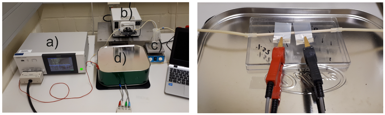
3.3. Setup and Procedure

The results were obtained in a small test setup (Figure 2). The solution, which is measured, is presented in a beaker and the opening of the beaker is covered with a PARAFILM ^® “M” (Bemis, Chicago, IL, USA) sealing film to avoid evaporation effects during the measurement. This solution is transported by an ISMATEC MC-MS CA4/6 (ISMATEC, Wertheim, Germany) peristaltic pump through the ceramic reactor in a circuit. In this testing setup, a DEGUSSIT AL23 (KYOCERA, Mannheim, Germany) tube, made of alumina with an outer diameter of 3 mm and an inner diameter of 1.6 mm served as the reactor. Furthermore, two different glass tubes (Hilgenberg, Malsfeld, Germany) with an outer diameter of 2 mm and an inner diameter of 1 mm or 1.6 mm were used for the investigation of the influence of the wall thickness. During measurement the testing solution is stirred by an IDL MEA30 magnetic stirrer (IDL, Nidderau, Germany). The electrodes are glued on the outer wall of the ceramic tube and electrically connected with the HIOKI IM3536 LCR—Meter (HIOKI E.E. Corporation, Ueda, Japan). The used schematic measuring cell is depicted in Figure 1b. This type of tubular cells are common for flowing systems [3,17]. The whole setup is placed in a Faraday cage. Two measuring methods are used: frequency sweep measurement and interval measurement at one specific frequency. First, sweep measurements were performed to determine the influence of frequency and salt concentration on the impedance. The frequency was varied from 1000 Hz to 8 MHz and repeated several times for each concentration. The concentration of the cerium nitrate solution was increased from zero (pure deionized water) to one mol/L. The different concentration levels are shown in

Table 1. Different concentration levels of cerium nitrate for the sweep measurements.

solution number	1	2	3	4	5	6	7	8	9
concentration /mol/L	0	0.001	0.005	0.01	0.02	0.05	0.1	0.2	1
abs. error /mmol/L	0	0.0013	0.063	0.13	0.25	0.61	1.12	2.24	5.10
rel. error ± /%	0	0.13	1.26	1.26	1.25	1.23	1.19	1.12	0.51

. Furthermore, tube-material, electrode-material, electrode distance and the electrode area are varied.

Table 2. Electrode configuration.

Designation	Tube-Material	Electrode -Material	Distance /mm	Width /mm	L /mm
Geo1	alumina	aluminum	5	5	15
Geo2	alumina	aluminum	10	5	20
Geo3	alumina	aluminum	20	5	30
Geo4	alumina	aluminum	5	10	25
Geo5	alumina	aluminum	10	10	30
Geo6	alumina	aluminum	20	10	40
Geo7	alumina	aluminum	5	20	45
Geo8	alumina	aluminum	10	20	50
Geo9	alumina	aluminum	20	20	60
Geo10	alumina	aluminum	10	15	40
GT0.2	glass	aluminum	5	20	45
GT0.5	glass	aluminum	5	20	45

shows the different used electrode configuration. Based on these measurements, the frequency for the interval measurements was localized. At this measurements the change of the impedance are determined by variation of the concentration. For the interval measurement, 5 mL of pure deionized water was used as a template and then 1 mL of a certain concentration was added every minute. An exemplary titration process is shown in

Table 3. Exemplary titration process.

Titration Step	Titration Volume /mL	Concentration /mol/L	Abs. Concentration /mol/L	Rel. Error ± /%
0	5	0	0	0
1	1	0.02	0.00333	1.48
2	1	0.04	0.00857	1.49
3	1	0.04	0.0125	1.58
4	1	0.04	0.0156	1.66
5	1	0.06	0.02	1.70
6	1	0.06	0.0236	1.75
7	1	0.06	0.0267	1.81
8	1	0.06	0.0292	1.86
9	1	0.1	0.0343	1.87
10	1	0.1	0.0387	1.89
11	1	0.1	0.0425	1.92
12	1	0.1	0.0459	1.94
13	1	0.2	0.0544	1.90
14	1	0.2	0.0621	1.88
15	1	0.2	0.069	1.87
⋮	⋮	⋮	⋮	⋮

. The addition of the solution was realized with a 1000 µL Eppendorf Pipette (Eppendorf, Hamburg, Germany). The used water is a HPLC specific water from FISHER CHEMICAL (Fisher Scientific, Schwerte, Germany) and the used cerium nitrate was ordered from Carl Roth (Cer(III)-nitrate hexahydrate, Karlsruhe, Germany). The used ceria nanoparticles were obtained at Merck (Merck, Darmstadt, Germany).

The error for the different concentrations levels of cerium nitrate, depicted in Table 1 and the error for the titration process (Table 3) is calculated according to Gaussian error propagation.

4. Results and Discussion

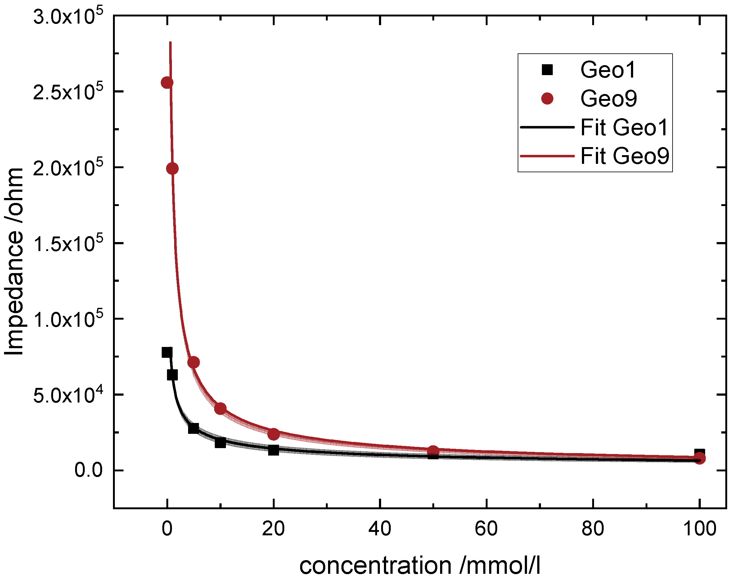
4.1. Fit and Modelling

Figure 3 represents the behavior of the equivalent circuit from Figure 1. For the evaluation of Equation (3), following values are used: $CP{E}_{cpl}=5.775·{10}^{-11}F$, ${\alpha }_{cpl}=0.75023$, $Q_m=1.029·{10}^{-15}F$, ${\alpha }_m=0.54822$, $C_x=6.986·{10}^{-14}F$ and $R_m=1.0646·{10}^7\Omega$. These values were obtained from fits of experimental data measuring water for electrode design Geo9 (see Table 2 Geo9).

The impedance modulus courses feature one region, were the influence of $R_m$ is measurable. If the resistance decrease ($R_m/10$), the flattened region moves to higher frequencies and the impedance is lower than $R_m$. If the resistance increase ($R_m·10$), the flattened region moves to lower frequencies and the impedance at this region is higher than $R_m$. The same behavior is shown by the phase angle $\theta$. With increasing values of $R_m$, the minimum of the phase angle shifts to lower frequencies and the value of the phase angle at the minimum increases. The changing phase minimum follows from the use of a CPE instead of an ideal capacitor in the equivalent circuit. Furthermore, it can be seen in Figure 3 that the phase minimum maps exactly to the frequency at which the impedance has the lowest slope. This is due to the fact that in the range in which $R_m$ dominates over the capacitance, the phase angle must approach zero, since a pure ohmic resistance has a phase angle of $0°$. A pure ideal capacitance, on the other hand, has a phase angle of $-90°$ and thus a small influence on the capacitance. This modeling shows the high ability to distinguish different concentrations of electrolytes with the described measuring cell, because of the decreasing resistance of the electrolyte by increasing concentration. For this calculation, the assumption was made that the capacitance of water and electrolyte is constant and equal, because of the constant electrode design. This does not correspond to reality but this assumption is considered practical. The focus for this examination is on the frequency range where the conductivity of the solution dominates over the capacitance, to distinguish different electrolyte concentrations. Therefore, the frequency range where the capacitance dominates can be neglected.

4.2. Measurements with Alumina Tubes as Reactor

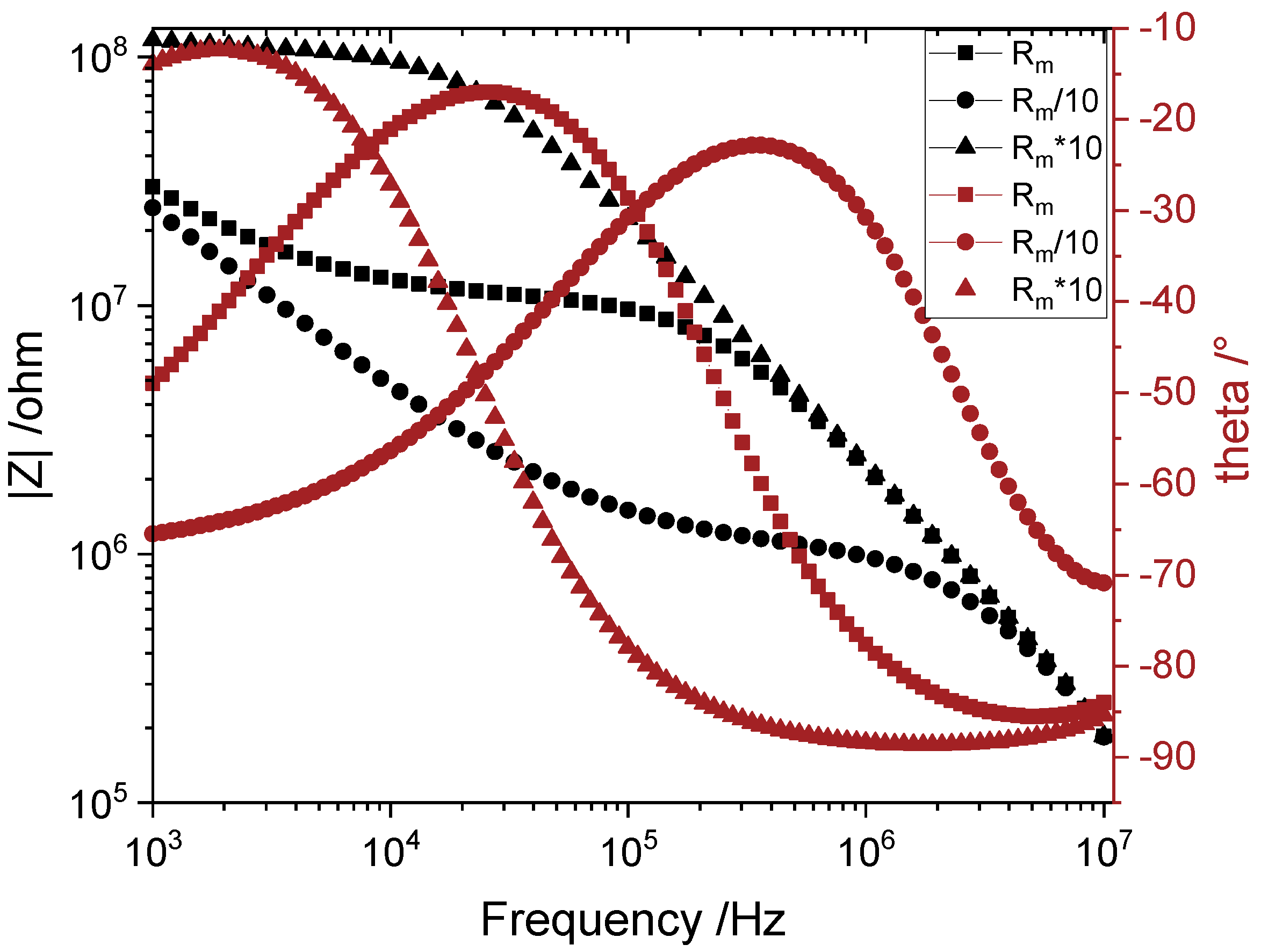
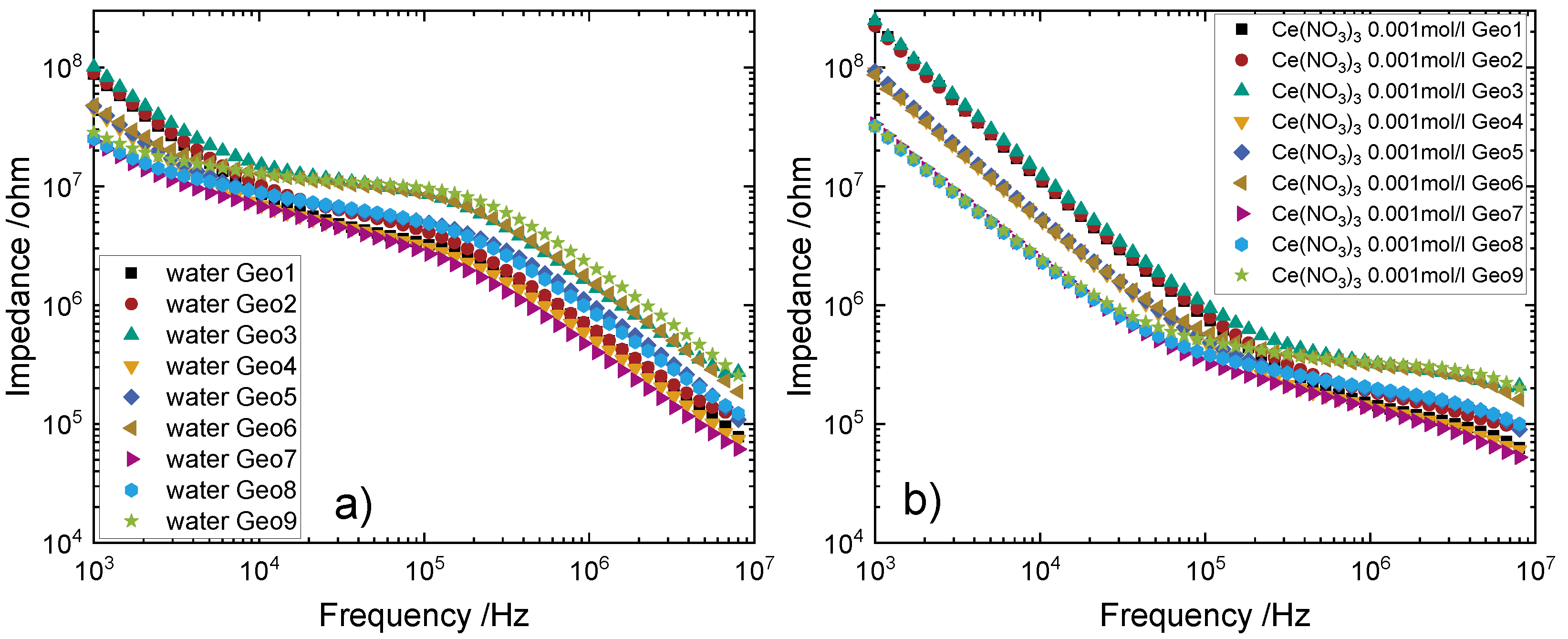
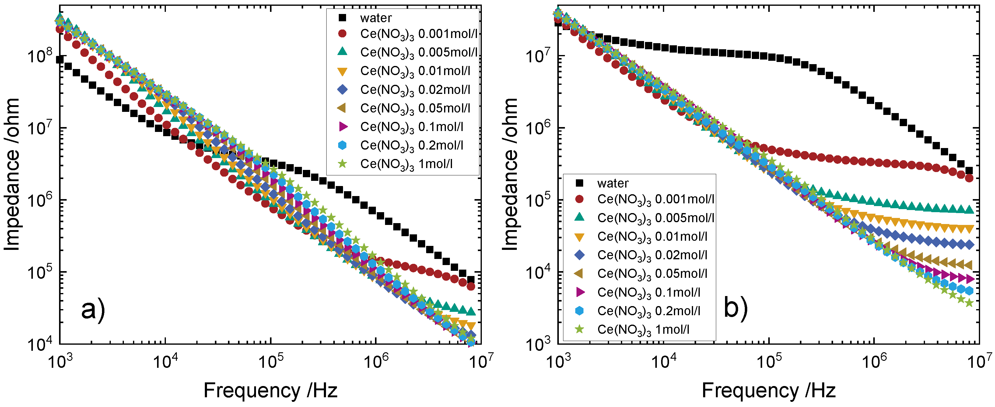
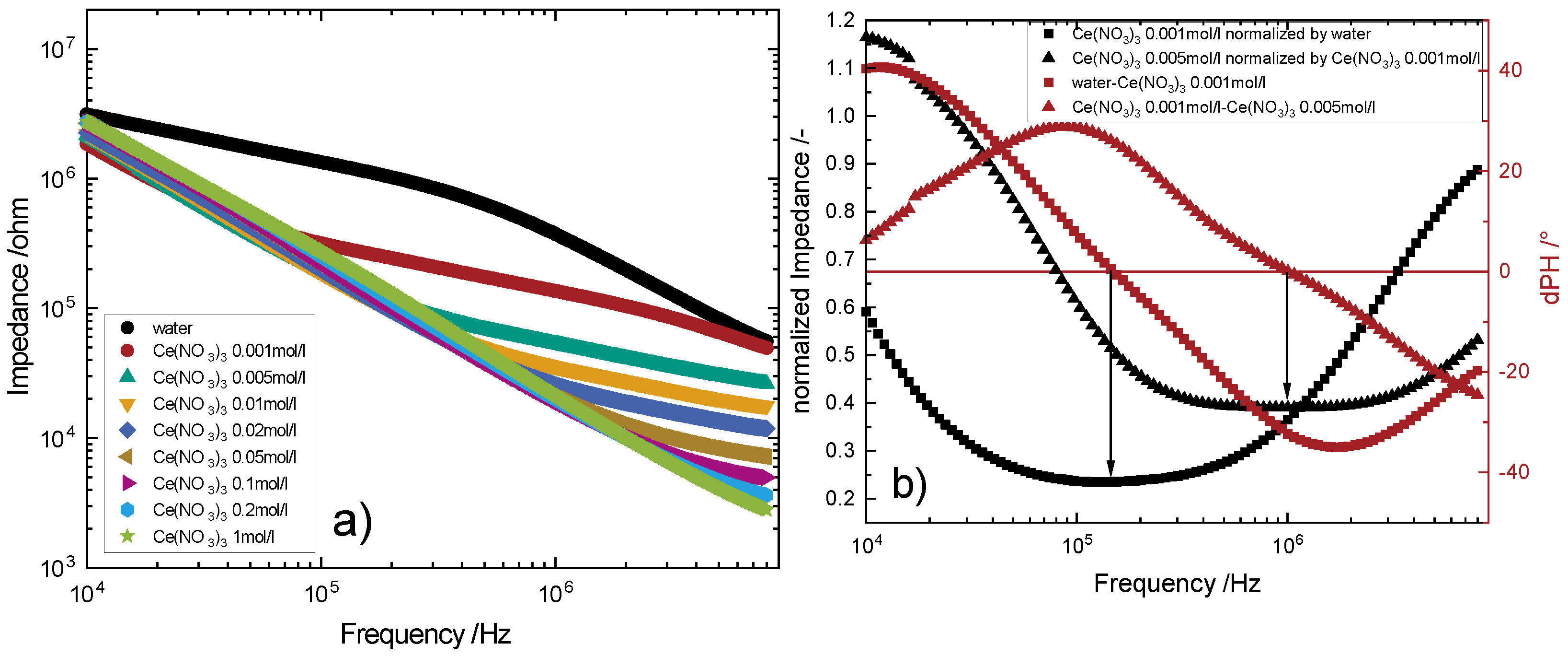
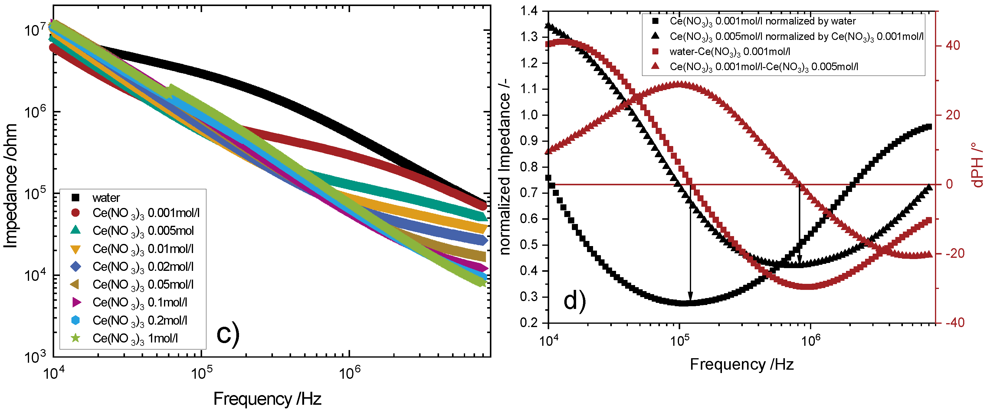
4.2.1. Sweep Measurements

Figure 4 shows the change of the impedance at different electrode designs with increasing frequency. The left diagram (a) represents water and the right diagram (b) cerium nitrate solution of 0.001 mol/L for nine different electrode designs. For all of them the impedance of water can divided in three parts. First, the impedance decreases linear, in this double logarithm diagram, with increasing frequency. Then a flattened curve is observed, in this part the conductivity of the fluid predominates compared to the capacitance. Finally a linear decrease of the impedance of water with increasing frequency. This result follows the calculated curves in Figure 3.

This nine electrode designs are different in the electrode distance and electrode width. The designs one to three have the same electrode width (5 mm) and the electrode distance doubles twice from 5 to 10 and to 20 mm. Designs four to six have a electrode width of 10 mm and distances of 5, 10 and 20 mm. Similar to this, designs seven to nine have a electrode width of 20 mm and distances of 5, 10 and 20 mm, as mentioned in Table 2. In the first linear decreasing part the electrode width predominates compared to the electrode distance. This is evident because the impedance of Geo1-3 lie on top of each other. The same applies to Geo4-6 and Geo7-9. In the second part, the flattening one, however, the impedance lie on top of each other, which have the same electrode distances. In the third sloping part, the impedance with the same electrode widths lie on top of each other. In addition, two further statements about the influence of electrode spacing and width can be made here. First, the larger the electrode spacing, the more the curve flattens in the middle part. This means, concerning to the equivalent circuit, that the influence of the capacitance (${CPE}_m$) decreases in comparison to the resistance of the liquid ($R_m$) and is therefore better suited to determine the resistance or the conductivity of the liquid. Secondly, it can be seen that with a larger electrode width, the middle part shifts to lower frequencies and the frequency span becomes larger. This has the advantage that a wider frequency range is available for the measurements. The right diagram (b) with the cerium nitrate solution is similar to the curves of water, with small differences. The overall impedance changes in all three parts. In the flattening part, the overall impedance is lower than that of water by more than a factor of 10. This is due to the fact that in this part the ohmic resistance $R_m$ predominates over the capacitance. By increasing the conductivity of the fluid, which was achieved here by increasing or adding the cerium nitrate salt, $R_m$ decreases according to Equation (4) and thus the overall impedance according to Equation (3) also decreases. Another point to add is, that the flattened part shifts to higher frequencies for cerium nitrate compared to water. The falling first and third part of the curve is not relevant for further consideration and is therefore not described further here.

Figure 5 shows the influence of the electrode design on the distinguishability of differently concentrated cerium nitrate solutions. The left (a) diagram represents the smallest investigated electrode design Geo1 with 5 mm distance and 5 mm width. The right diagram (b) shows the biggest investigated electrode design Geo9 with 20 mm distance and 20 mm width. The impedance of Geo1 to Geo9 changes in different ways. As long as the course of the impedance decreases linearly, in this double logarithmic diagram, the impedance of Geo9 is smaller than that of Geo1. This is due to the fact that the electrode width of Geo9 increases in comparison to Geo1, which according to Equation (5) leads to an increase of ${CPE}_{cpl}$ and thus to a reduction of the impedance Z. On the other hand, in the flattening region where $R_m$ dominates over capacitance, the impedance of Geo9 is higher than that of Geo1. This is due to the increase in the total cell length l, which was achieved in Geo9 by increasing the electrode distance and width. This increases the resistance $R_m$ and leads to a higher overall impedance. This curve can be observed not only for water, but also for all other salt concentrations. The difference is that the flattening section shifts to higher frequencies with increasing salt concentration or decreasing resistance. This is due to the frequency dependence of the capacitive resistances which tend towards infinity at a frequency of zero and towards zero for a frequency of infinity. Another difference between Geo1 and Geo9 is, that the flattened part of the course is bigger for all differently concentrations and started at lower frequencies at Geo9 than at Geo1. In addition, it can be observed that the impedance of the cerium nitrate solutions at Geo1 overlie or even cross each other over a large frequency range, making it impossible to distinguish the individual concentrations. Only the concentration of 0.001 mol/L and water can be distinguished between a frequency of about 100 kHz and 1 MHz. However, since in this range also the high concentrations around 1 mol/L intersect the range it is important to know the initial maximum concentration to be able to measure a change of the concentration later. In comparison with Geo9, however, this phenomenon of crossing and overlapping the impedance of cerium nitrate solutions occurs at lower frequencies. This, and the wider flat part of the impedance, resulting in better discrimination between concentrations over a wider frequency range. However, again, the initial concentration must be known. Furthermore, it can be observed with Geo9 that the distinguishability between the concentration curves shown here is shifted to higher frequencies with increasing concentration.

In comparison to the calculated equivalent circuit (Figure 3) there is a difference at lower frequencies. In the measurements, pure deionized water and the cerium nitrate salt solution have not the same impedance at low frequencies, but if the difference between water and the salt solution is only in the conductance, the impedance shout be equal like in the calculation. However, there is a difference between water and the salt solutions and moreover there are small differences between the salt solutions with different concentrations at Geo9 and bigger differences at Geo1. This follows from the ideal assumption, as already discussed above. This point shows, that the capacity of the electrolyte (${CPE}_m$) has also an influence on the behavior of the impedance. Nevertheless, the capacity influence is negligible at the focused frequency-range, where the resistance predominate. The same differences between measurement and calculation were observed from Blume et al. [18] for a KCl—solution before. Therefore it’s necessary to know the frequency-range for each cell geometry in which the resistance of the fluid predominates.

Figure 6 shows the impedance versus concentration for Geo1 and Geo9. This are the same measurements as in Figure 5 at 8 MHz. The dots are the measured impedance and the line are the fitted impedance. As can be seen here, a continuous curve of impedance as a function of concentration can be generated with a few sweep measurements. This has the advantage that a reference curve can be prepared with a few measurements in order to determine the concentration by means of impedance in subsequent titration experiments.

Figure 6. Calibration−Fit for Geo1 and Geo9 with statistical consideration. The impedance measurements were made at 8 MHz. The fitting parameter for the asymptotic-fit are shown in

Table 4. Fitting Parameter for fit Geo1 and Geo9.

Label	Equation	a	b	R${}^2$
Geo1	$y=a·x^b$	62,231.2 ± 2400	−0.488 ± 0.031	0.988
Geo9	$y=a·x^b$	199,725.9 ± 2598.7	−0.678 ± 0.016	0.998

.

Figure 6. Calibration−Fit for Geo1 and Geo9 with statistical consideration. The impedance measurements were made at 8 MHz. The fitting parameter for the asymptotic-fit are shown in Table 4.

In summary, the following statements can be made about the two influencing variables of the electrodes (width and distance).

• The larger the electrode width, the more distinguishable is the measurement at lower concentrations for cerium nitrate.
• Higher distances between the electrodes lead to more distinguishable measurements at lower concentrations and till higher concentrations.

Based on these findings, the most accurate results up to very high concentrations should be obtained with the largest possible electrodes having a large distance.

4.2.2. Titration Measurements

Figure 7 represents titration measurements of cerium nitrate salt solutions. The left diagram shows electrode design Geo6, this reactor has aluminum electrodes with electrode width of 10 mm and a distance of 20 mm. The right diagram shows electrode design Geo10, with aluminum electrodes with a width of 15 mm and a distance of 10 mm. This two electrode geometries are selected for the titration measurements, because of the application on the real CHTS-plant. Currently, only electrode geometries with a maximum length of 50 mm are possible. All measurements were performed at 8 MHz. As a comparison, the blue dots represents the Impedance values of the sweep measurements at 8 MHz. At the left diagram, the black squares and red circles are measured with the same titration procedure. The green triangle upwards and orange triangle down represents another titration procedure. It is noticeable that the green and yellow measurement three and four are equal over the hole concentration range, but measurement one and two are only identical at a concentration above 0.1 mol/L. At lower concentrations, especially between zero and 0.05 mol/L there are some measurement points with a larger difference.

This diagram shows that the measurements are reproducible at concentrations above 0.05 mol/L. Each measuring point at Figure 7 shows the average of one minute of measuring which includes about 60 measuring points and the error bars are really close (≈0.1–0.6%). By the aspect, that the impedance measurement at lower concentration are more sensitive it is not aberrant that the differences between each measurement are higher than at high concentrations. A deviation had to be assumed due to measurement inaccuracies, mainly errors during titration and preparation of the batch. It should be emphasized that the impedance values of the sweep measurements are fairly close to the titration values (

Table 5. Error between titration measurement and sweep measurement of Geo6.

Concentration /mol/L	Rel. Error Concentration/%	Rel. Error Impedance/%	Rel. Error Solution/%
0	0	2.4	0
0.02	0	1.5	1.7
0.04	3.4	2.3	1.9
0.06	4.7	0.8	1.9
0.08	3.4	1.3	1.9
0.2	0.6	4.0	1.3

). Therefore, in order to determine the concentration of a flowing salt solution, it is important to create a calibration line first. Similar to the left diagram, the black squares and red circles at the right diagram represents the same titration procedure. The green and yellow triangles show a different titration procedure to illustrate the behavior for bigger concentration ranges. With different titration procedures, the same impedance values are obtained for the respective concentrations. Therefore, it is irrelevant whether the concentration increases or decreases, the impedance value for the respective concentrations is the same. The calibration measurements for reactor Geo10 has small differences to the titration measurement at high concentrations and higher differences at lower concentrations (

Table 6. Error between titration measurement and sweep measurement of Geo10.

Concentration /mol/L	Rel. Error Concentration/%	Rel. Error Impedance/%	Rel. Error Solution/%
0	0	0.3	0
0.02	0	15.2	1.7
0.04	3.4	13.4	1.9
0.06	5.4	5.5	1.9
0.08	3.4	6.9	1.9
0.1	2.8	7.6	1.6
0.2	1.8	7.9	1.3
0.5	0.2	7.3	1.2

). The error bars follow this observation. After adding of solution to the testing volume, a sudden increase of the concentration leads to the larger error bars at the individual measuring points in case of high sensitivity at low concentrations. By stirring the solution, a stable measurement signal is obtained after a few seconds. The relative concentration change is smaller at high concentrations compared to low concentrations, thus the error bars are smaller at high concentrations.

4.2.3. Ternary Systems

Figure 8 shows the influence of the product of the CHTS-process (ceria nanoparticles) on the impedance. Water is compared with a water-ceria-suspension (CeO${}_2$) and a cerium nitrate solution with the suspension of the cerium nitrate solution and CeO${}_2$. In addition, the difference in distinguishability for two different cell geometries (Geo1, Geo9) is shown. No differences between water and the corresponding suspension of water and ceria can be observed, either for the geometry on the left side nor on the right side. In Geo9, moreover, no influence of a higher concentration of CeO${}_2$ nanoparticles is visible. This statement can also be made for the cerium nitrate suspension and the cerium nitrate solution. This corresponds to the intensity of the measurement. By adding a metal oxide nanoparticle to water or to a metal salt solution, the conductivity of the solution or suspension should not change, since the oxide does not dissociate into ions. In addition, it is well known that ceramics with their ionic bonds act as electrical insulators. The errors of the measurement between the solutions and the suspensions depend on the frequencies which are maximum ±4%. For this purpose, the measurements of the suspensions were normalized with the measurements of the solutions. As mentioned before, larger electrode areas leads to smaller impedances, a bigger frequency-range to distinguish different salt concentrations and the ability to use smaller frequencies for the measurement, like Geo9 compared to Geo1. This observation allows with defined reactant concentration to determine the conversion of the reaction by measuring the residual concentration of the salt, because the ceria nanoparticles do not change the impedance. Thus, this method has the ability to immediately, continuously and directly determine the reaction conversion in the plant. Furthermore, embedded in a control loop it would be possible to control the conversion by varying the process parameters. This eliminate the need for chemical analysis of the product.

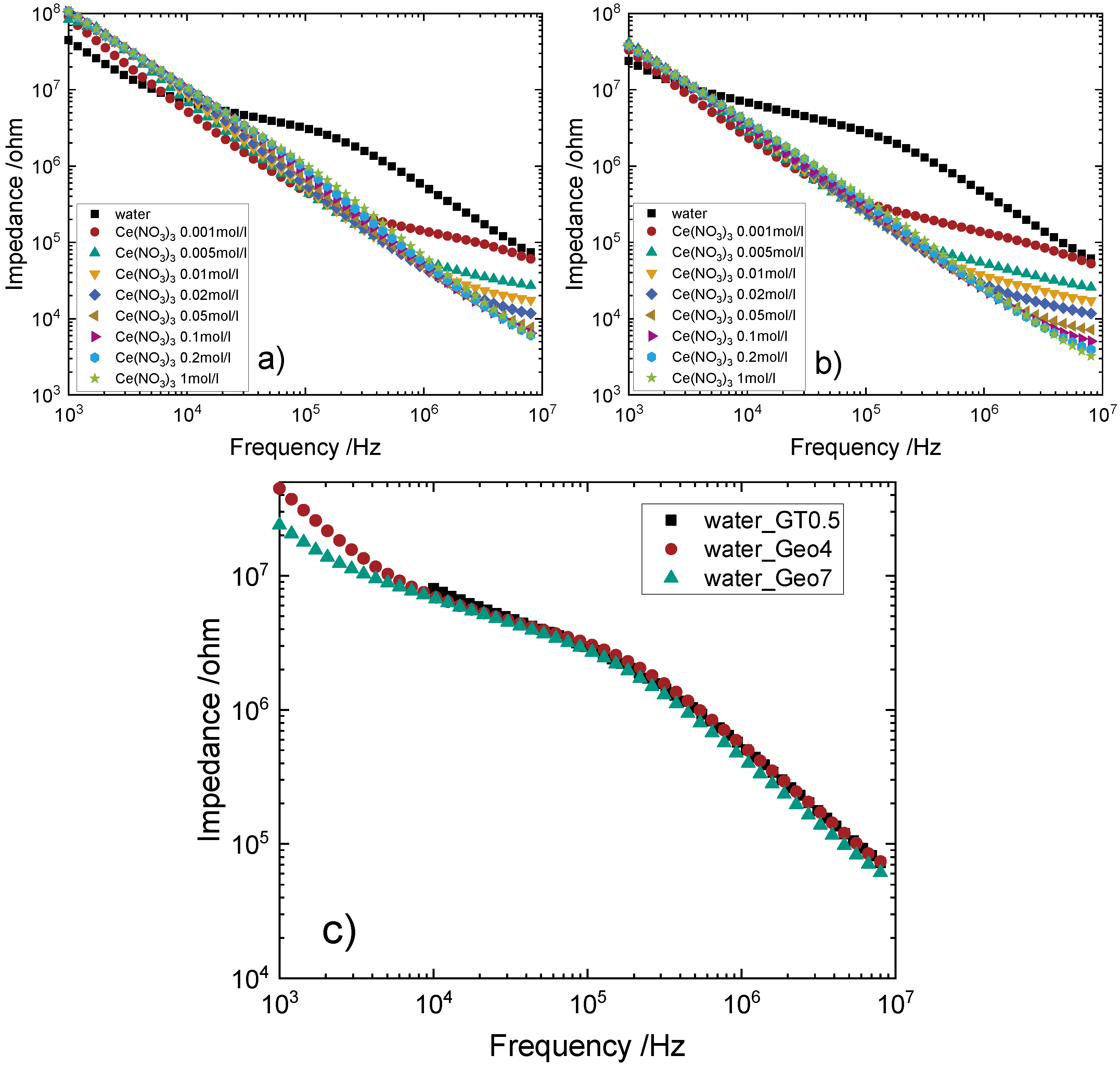
4.3. Measurements with Glass Tubes as Reactor

The aforementioned results were generated with alumina tubes. Figure 9 compares two different wall thicknesses of glass tubes. Glass tubes were used for the variation of the wall thickness, because no alumina tubes are commercially available in which the outer diameter is constant and the inner diameter, i.e., the wall thickness, is varied. The wall thickness of the used tube has a great influence on the behavior of the measuring cell, because of the change in the capacity ${CPE}_{cpl}$ in Equation (3). The diagram (a) and (b) shows the behavior of the measuring cell with a glass thickness of 0.2 mm and measuring cell (c) and (d) represents a wall thickness of 0.5 mm. The two diagrams (a) and (c) differ in so far as, with increasing wall thickness the overall impedance increase, which can be explained with Equation (5). With increasing of $r_i$ and a constant value of $r_o$, the capacitance ${CPE}_{cpl}$ is also increasing and the overall impedance decreases corresponding to Equation (3). An other difference is the distinctness of concentrations of Ce(NO${}_3$)${}_3$ solutions. There is a bigger gap between each course at diagram (a) at high frequencies, than at diagram (c). Therefore, the distinctness of concentrations at high frequencies increases with decreasing wall-thickness [19,20]. However, a disadvantage at high frequencies is, that there is no difference of the impedance values at lower concentrations between pure water and 0.001 mol/L. The biggest difference between the impedance values at low concentrations shifts to lower frequencies. The diagrams (b) and (d) shows, at the left Y-axes normalized impedance and at the right Y-axes phase shift, two measurements of the corresponding glass-tube-reactor from diagram (a) and (c). Here, the Ce(NO${}_3$)${}_3$ solution with the concentration of 0.001 mol/L is normalized by the water spectrum. In order to this, the Ce(NO${}_3$)${}_3$ solution with the concentration of 0.005 mol/L is normalized by the cerium nitrate solution of 0.001 mol/L. Through this normalization, a minimum is obtained which represents the maximum difference in impedance between two concentration solutions. The frequency at which this maximum difference occurs is also the frequency at which the phase difference between the respective concentrations becomes zero. This makes it possible to determine a suitable frequency at which the difference in impedance is maximized and the discrimination between the individual concentrations is also maximized. For example, the example in Figure 9 shows that a change in concentration from zero to 0.001 mol/L of cerium nitrate is most appropriately measured at a frequency of about $1.5·{10}^5$ Hz, while a change in concentration from 0.001 to 0.005 mol/L is most appropriately determined at a frequency of $1·{10}^6$ Hz. In order to a continuous measurement for a large concentration range, it is necessary to use more than one frequency to get high distinguishability for the hole concentrations range. To sum up, thin wall thicknesses are more suitable for the indirect concentration measurements of electrolytes with a C${}^4$D-Sensor, because of the higher distinguishability.

Another factor influencing the overall impedance is the electrical permittivity, as can be seen in Equation (5). Therefore, two different electrode geometries are shown in Figure 10a,b, using an alumina tube as a reactor. As shown in Table 2, the outer diameter of the alumina tubes is 3 mm, which is larger than the outer diameter of the glass tubes, which is 2 mm. In addition, the wall thickness of 0.2 mm and 0.5 mm is smaller for the glass tubes than for the alumina tubes with 0.7 mm. Since there are no glass tubes with the same dimensions as the aluminum oxide tubes and vice versa commercially available, not optimal comparisons are used here. Nevertheless, the influence on the overall impedance of the permittivity can be obtained from this. In Figure 9, it can be observed that a lower wall thickness lowers the impedance and increases the distinguishability of the individual electrolyte solutions. In Figure 10c the electrode geometries of Geo4, Geo7 and GT0.5 are compared for water. All three have an electrode spacing of 5 mm. As shown in Section 4.2.1, the three curves therefore overlap in the middle frequency range, since the conductivity of the water outweighs the capacitance here. Due to the different electrode areas, the curves do not overlap in the low and high frequency range. The impedance curve of the GT0.5 glass tube shows three different parameters in contrast to the aluminum oxide tubes. The wall thickness of the glass tube, the electrode area and the permittivity. Geo4 should have a significantly higher impedance in the low and high frequency range due to the higher wall thickness and the smaller electrode area. However, this cannot be seen. Due to the higher permittivity of alumina (8–10 at 1 MHz) in contrast to glass (4–8 at 1 MHz), the impedance drops in these two frequency ranges and is comparable to GT0.5. This shows the influence of the permittivity of the material of the insulation tube on the impedance. This can also be understood by means of Equations (3) and (5).

5. Conclusions

In this work, a possible method for determining the concentration of cerium nitrate in a flowing system using impedance spectroscopy and the application of C${}^4$D Sensors was described. For this purpose, the influences of the electrode distance and -width, as well as the wall thickness of the tube and the material of the tube on the impedance were investigated. It was found that with a larger electrode width and a larger electrode distance, the distinguishability of individual cerium nitrate concentrations increases. In addition, the maximum difference in impedance between two different salt concentrations was found to shift to higher frequencies with increasing concentration. It has also been shown that a reduction in the wall thickness of the tube leads to higher discrimination, as does the use of glass instead of aluminum oxide as an insulating material. In this work, with electrodes of 20 mm width and 20 mm spacing, cerium nitrate could be distinguished in a frequency range of $1·{10}^5$–$8·{10}^6$ Hz in a concentration of 0–1 mol/L. Therefore, the impedance spectroscopy combined with C${}^4$D Sensors is a powerful method to determine concentration changes in flowing systems. In this case, it could be a possible method to detect chemical reactions in continuous processes, especially for the continuous hydrothermal syntheses, which were developed in this research project [21].

References

1. Hall, J.L.; Gibson, J.A. High-Frequency Titration. Anal. Chem. 1951, 23, 966–970. [Google Scholar] [CrossRef]
2. Hall, J.L. High-Frequency Titration: Theoretical and Practical Aspects. Anal. Chem. 1952, 24, 1236–1240. [Google Scholar] [CrossRef]
3. Zemann, A.J.; Schnell, E.; Volgger, D.; Bonn, G.K. Contactless conductivity detection for capillary electrophoresis. Anal. Chem. 1998, 70, 563–567. [Google Scholar] [CrossRef] [PubMed]
4. Kubáň, P.; Hauser, P.C. 20th anniversary of axial capacitively coupled contactless conductivity detection in capillary electrophoresis. TrAC Trends Anal. Chem. 2018, 102, 311–321. [Google Scholar] [CrossRef]
5. Kubán, P.; Hauser, P.C. Ten years of axial capacitively coupled contactless conductivity detection for CZE—A review. Electrophoresis 2009, 30, 176–188. [Google Scholar] [CrossRef] [PubMed]
6. Kubáň, P.; Hauser, P.C. Contactless Conductivity Detection in Capillary Electrophoresis: A Review. Electroanalysis 2004, 16, 2009–2021. [Google Scholar] [CrossRef]
7. Kubán, P.; Hauser, P.C. A review of the recent achievements in capacitively coupled contactless conductivity detection. Anal. Chim. Acta 2008, 607, 15–29. [Google Scholar] [CrossRef] [PubMed]
8. Hauser, P.C.; Kubáň, P. Capacitively coupled contactless conductivity detection for analytical techniques—Developments from 2018 to 2020. J. Chromatogr. A 2020, 1632, 461616. [Google Scholar] [CrossRef] [PubMed]
9. Cahill, B.P. Optimization of an impedance sensor for droplet-based microfluidic systems. In Smart Sensors, Actuators, and MEMS V; Schmid, U., Sánchez-Rojas, J.L., Leester-Schaedel, M., Eds.; SPIE Proceedings; SPIE: New York, NY, USA, 2011; p. 80660F. [Google Scholar] [CrossRef]
10. Tůma, P.; Opekar, F.; Štulík, K. A contactless conductivity detector for capillary electrophoresis: Effects of the detection cell geometry on the detector performance. Electrophoresis 2002, 23, 3718–3724. [Google Scholar] [CrossRef]
11. Türk, M. Design metalloxidischer Nanopartikel mittels kontinuierlicher hydrothermaler Synthese. Chem. Ing. Tech. 2018, 90, 436–442. [Google Scholar] [CrossRef]
12. Brito-Neto, J.G.A.; Fracassi da Silva, J.A.; Blanes, L.; do Lago, C.L. Understanding Capacitively Coupled Contactless Conductivity Detection in Capillary and Microchip Electrophoresis. Part 2. Peak Shape, Stray Capacitance, Noise, and Actual Electronics. Electroanalysis 2005, 17, 1207–1214. [Google Scholar] [CrossRef]
13. Gaš, B.; Zuska, J.; Coufal, P.; van de Goor, T. Optimization of the high-frequency contactless conductivity detector for capillary electrophoresis. Electrophoresis 2002, 23, 3520–3527. [Google Scholar] [CrossRef]
14. Opekar, F.; Tůma, P.; Stulík, K. Contactless impedance sensors and their application to flow measurements. Sensors 2013, 13, 2786–2801. [Google Scholar] [CrossRef] [PubMed] [Green Version]
15. Novotný, M.; Opekar, F.; Štulík, K. The Effects of the Electrode System Geometry on the Properties of Contactless Conductivity Detectors for Capillary Electrophoresis. Electroanalysis 2005, 17, 1181–1186. [Google Scholar] [CrossRef]
16. Barsoukov, E.; Macdonald, J.R. Impedance Spectroscopy; Wiley: Hoboken, NJ, USA, 2005. [Google Scholar] [CrossRef]
17. Fracassi da Silva, J.A.; do Lago, C.L. An Oscillometric Detector for Capillary Electrophoresis. Anal. Chem. 1998, 70, 4339–4343. [Google Scholar] [CrossRef]
18. Blume, S.O.; Ben-Mrad, R.; Sullivan, P.E. Characterization of coplanar electrode structures for microfluidic-based impedance spectroscopy. Sens. Actuators B Chem. 2015, 218, 261–270. [Google Scholar] [CrossRef]
19. Tanyanyiwa, J.; Hauser, P.C. High-voltage capacitively coupled contactless conductivity detection for microchip capillary electrophoresis. Anal. Chem. 2002, 74, 6378–6382. [Google Scholar] [CrossRef] [PubMed]
20. Mark, J.J.P.; Coufal, P.; Opekar, F.; Matysik, F.M. Comparison of the performance characteristics of two tubular contactless conductivity detectors with different dimensions and application in conjunction with HPLC. Anal. Bioanal. Chem. 2011, 401, 1669–1676. [Google Scholar] [CrossRef] [PubMed]
21. Schüßler, C.; Zürn, M.; Hanemann, T.; Türk, M. Überwachung der kontinuierlichen hydrothermalen Synthese mittels Impedanzspektroskopie. Chem. Ing. Tech. 2021, 38, 242. [Google Scholar] [CrossRef]
Figure 1. (a): Equivalent circuit of the impedance cell with the following components: ( C P E c p l ) (cpl: coupled layer) represents the two electrodes, R m represents the resistance of the medium, C P E m represents the capacitive resistance of the medium and C x represents the stray capacitance between the two electrodes. (b): Scheme of the impedance cell.
Processes 10 02075 g001
Figure 2. (left): Test setup with the (a) HIOKI IM3536 LCR meter, (b) peristaltic pump, (c) magnetic stirrer and (d) the test cell, covered in the faraday cage. (right): test cell.
Processes 10 02075 g002
Figure 3. Bode−Plot for three different R m . Left Y−axis represents absolute Impedance versus frequency and the right Y−axis shows the phase angle theta versus frequency.
Processes 10 02075 g003
Figure 4. Impedance over frequency for deionized water (a) and cerium nitrate (b) with different electrode geometries, which are mentioned in Table 2.
Processes 10 02075 g004
Figure 5. Impedance over frequency for deionized water and cerium nitrate with different concentrations. (a), Geo1 (5 mm distance, 5 mm width) and (b), Geo9 (20 mm distance, 20 mm width).
Processes 10 02075 g005
Figure 7. Impedance versus concentration of titration measurements. (a) electrode design Geo6 and (b) reactor electrode design Geo10. Every titration measurements were measured at 8 MHz.
Processes 10 02075 g007
Figure 8. Impedance versus frequency for deionized water, cerium nitrate with a concentration of 0.001 mol/L and ternary systems of water, cerium nitrate and ceria. (a) electrode design Geo1 (5 mm distance, 5 mm width) and (b) electrode design Geo9 (20 mm distance, 20 mm width).
Processes 10 02075 g008
Figure 9. (a,c) Impedance over frequency for deionized water and cerium nitrate with different concentrations. (b,d) normalized impedance and phase shift over frequency. (a,b), glass-tube-reactor with a wall thickness of 0.2 mm and (c,d) glass-tube-reactor with a wall thickness of 0.5 mm. With tubular electrodes of 5 mm distance and 20 mm width for both glass-tube-reactors.
Processes 10 02075 g009aProcesses 10 02075 g009b
Figure 10. Impedance over frequency for deionized water and cerium nitrate with different concentrations. (a) Geo4 with an electrode width of 10 mm and a distance of 5 mm, (b) Geo7 with an electrode width of 20 mm and a distance of 5 mm. At both electrode designs, alumina tube are used. (c) Comparison of water with different electrode geometries, see Table 2 and different tube materials. Black square, glass tube are used, red circles and green triangle alumina tube are used.
Processes 10 02075 g010