
Remote Wind Farm Path Planning for Patrol Robot Based on the Hybrid Optimization Algorithm
by
 ,
,
Luobing Chen
1, 
Zhiqiang Hu
2,*,
Fangfang Zhang
1,*,
Zhongjin Guo
3,
Kun Jiang
4,
Changchun Pan
5 and
Wei Ding
6 1
School of Information and Automation Engineering, Qilu University of Technology (Shandong Academy of Sciences), Jinan 250353, China
2
College of Mechanical and Architectural Engineering, Taishan University, Taian 271000, China
3
School of Mathematics and Statistics, Taishan University, Taian 271000, China
4
College of Mechanical and Control Engineering, Guilin University of Technology, Guilin 541000, China
5
Key Laboratory of Navigation and Location Based Services, Shanghai Jiao Tong University, Shanghai 200030, China
6
Shandong Computer Science Center (National Supercomputer Center in Jinan), Qilu University of Technology (Shandong Academy of Sciences), Jinan 250353, China
*
Authors to whom correspondence should be addressed.
Processes 2022, 10(10), 2101; https://doi.org/10.3390/pr10102101
Submission received: 8 July 2022
/
Revised: 12 October 2022
/
Accepted: 13 October 2022
/
Published: 17 October 2022
(This article belongs to the Special Issue Modelling, Monitoring, Control and Optimization for Complex Industrial Processes)
Abstract
:Globally, wind power plays a leading role in the renewable energy industry. In order to ensure the normal operation of a wind farm, the staff will regularly check the equipment of the wind farm. However, manual inspection has some disadvantages, such as heavy workload, low efficiency and easy misjudgment. In order to realize automation, intelligence and high efficiency of inspection work, inspection robots are introduced into wind farms to replace manual inspections. Path planning is the prerequisite for an intelligent inspection robot to complete inspection tasks. In order to ensure that the robot can take the shortest path in the inspection process and avoid the detected obstacles at the same time, a new path-planning algorithm is proposed. The path-planning algorithm is based on the chaotic neural network and genetic algorithm. First, the chaotic neural network is used for the first step of path planning. The planning results are encoded into chromosomes to replace the individuals with the worst fitness in the genetic algorithm population. Then, according to the principle of survival of the fittest, the population is selected, hybridized, varied and guided to cyclic evolution to obtain the new path. The shortest path obtained by the algorithm can be used for the robot inspection of the wind farms in remote areas. The results show that the proposed new algorithm can generate a shorter inspection path than other algorithms.
1. Introduction
In recent years, power enterprises have been paying more attention to wind power generation, developing new energy power generation and promoting the sustainable development of the power generation industry [1,2]. Yet at the same time, the equipment used by wind farms is prone to malfunction when large-scale wind farms are affected by extreme operating environments, such as extremely high or low temperature, corrosion, and strong high pressure. Equipment failure causes a huge economic loss. Patrol inspection and maintenance of wind farms can reduce the probability of equipment failure, thereby avoiding some economic losses.
With the development of intelligent technology, inspection robots have been widely used at wind farms to complete inspection work. At present, wind farms have begun to reduce their number of inspection personnel. By using inspection robots to carry out intelligent inspections on the wind farm, inspection efficiency is improved and the safe operation of the wind farm is guaranteed. Global path planning is a prerequisite for an intelligent inspection robot to complete inspection tasks. Therefore, it is of great significance to study the global path planning of robot wind farm inspections.
Many scholars have discussed the path planning of wind farms for patrol robots and proposed a variety of algorithms. Path planning is essentially a traveling salesman problem. Generally, these algorithms can be divided into biology-based metaheuristic algorithms, physics-based metaheuristic algorithms, group-based metaheuristic algorithms and so on. In addition, there are hybrid algorithms that combine these methods [3,4], which are shown in Table 1.
For small-scale path-planning problems, a single algorithm [5,6,7] can quickly obtain the optimal solution. However, it is difficult to cope with large-scale and complicated structures. Therefore, the scholars proposed some hybrid algorithms. These algorithms can find high-quality approximate solutions to solve road-planning problems, such as hybrid algorithms based on genetic algorithms, analog annealing algorithms and other algorithms [10].
For reference [8], high quality initial solutions of genetic algorithms can improve problem-solving speed and even improve the quality of final solutions. For reference [9], the ant colony algorithm has strong robustness. The ant colony algorithm has fewer parameters and is easy to set up, so it is easy to apply to other combinatorial optimization problems. The algorithms proposed in [8,9] all involve the simulated annealing algorithm. However, the chaotic annealing mechanism of transient chaotic neural network (TCNN) is better than the traditional analog annealing algorithm in regard to global search capabilities and learning rates [11,12].
Based on the above discussions, we combine the advantages of genetic algorithms and TCNN, propose a hybrid optimization algorithm, and apply it to the path planning of a patrol robot. This algorithm can obtain a higher-quality path solution, thereby reducing the costs of wind farm operation and maintenance. The main contributions are as follows:
In order to optimize the patrol path of the wind farm in the remote area, a new hybrid optimization algorithm based on the chaotic neural network and genetic algorithm is proposed. To verify its effectiveness, the proposed algorithm is firstly applied to the traveling salesman problem, then compared with other algorithms. The simulation results show that the algorithm has better path search capabilities and can be extended to other related engineering fields, such as path planning for wind farms.
In path planning for wind farms, if there are some obstacles between any two adjacent wind farms that can be detoured around, the original distance is replaced with the detour length. The proposed algorithm can obtain a shorter patrol path than other algorithms. In this case, it is still an unconstrained problem.
In path planning for wind farms, if we consider the obstacles such as mountains and rivers that cannot be detoured around, or other constrained conditions, such as the inability of the patrol robot to move from one wind farm to the special wind farm, the model of path planning is established, and the proposed algorithm also obtains a shorter patrol path than other algorithms. In this case, it is, in essence, one constrained problem.
The content of this paper is arranged as follows: Section 2 introduces the patrol path model of wind farms. Section 3 introduces a new hybrid optimization algorithm and introduces the simulation experiment of the traveling salesman problem to verify the effectiveness of the proposed algorithm. In Section 4, we apply the proposed algorithm to the path planning for the patrol robot in remote areas. Section 5 summarizes the main work of this paper.
2. The Model of Path Planning
2.1. Path Planning
A redundant inspection path will cause the problems of heavy workload and low efficiency [13]. The location coordinates of each wind farm are known. A reasonable routing planning scheme must meet the following conditions:
Condition (1): Path length problem. The patrol robot visits each wind farm at a fixed position once, then returns to the original wind farm after the entire visit. Based on ensuring the effective completion of the inspection task, the patrol robot selects the optimal forward path to reduce the operation and maintenance cost of the wind farms.
Condition (2): If there is a barrier between the two wind farms, the robot can detour around the barrier from the current wind farm to the next wind farm.
Condition (3): If there are obstacles that cannot be detoured around between the two wind farms, the patrol robot will find other wind farms to ensure that the patrol task can be completed.
2.2. Objective Function
2.2.1. Constraints
The function corresponding to condition (1) is as follows:
where xi0 = xin, xin + 1 = xi1, W2 is the coupling coefficient corresponding to the constrained cost function. Condition (3) discussed in this paper is embodied in the form of algorithms. For example,
where p is the matrix that measures the obstacle between two points. pij stands for path condition from city i to city j, where 1 indicates that there is an obstacle, and 0 indicates that there is no obstacle. When the solution matrix dot multiplied by matrix p is 0, the scheme satisfies condition (3). The case for condition (2) is described in Section 4.1.
2.2.2. Objective Function
The essence of the wind farms inspection problem is the path-planning problem. The goal is to minimize the length of the patrol path. Assuming that the output xij is the order j of accessing the city i, the value of the output xij is initialized randomly. xij means that city i is visited on the jth order. For example,
where 1 indicates the arrival to the city, and 0 indicates no access to the city. x12 means city 1 is visited at the second time.
Then, the objective function corresponding to the problem is as follows:
where W1 is the coupling coefficient corresponding to the cost function of the path length, and dij is the distance between city i and city j, xi0 = xin, xin + 1 = xi1, W2 is the coupling coefficient corresponding to the constrained cost function.
3. The Proposed Hybrid Optimization Algorithm
3.1. Transient Chaotic Neural Network
Based on a Hopfield neural network, the self-feedback term with simulated annealing mechanism is added, which is called the transient chaotic neural network (TCNN). The dynamic equation is as follows:
where yi (t) is the internal state of neurons, xi (t) is the output of neurons, k is the damping factor of the neural diaphragm , α is a positive proportion parameter. It represents the effect of energy function on chaotic dynamics, , ε is the steepness parameter of the activation function , I0 is the positive parameter, zi (t) is the self-feedback connection weight, β is the annealing attenuation factor of zi (t).
A positive Lyapunov exponent indicates that the model has chaotic characteristics, and the larger the Lyapunov exponent, the stronger the degree of chaos. Lyapunov exponent is defined as follows:
Therefore, for the TCNN chaotic neuron model:
where
Set parameters: k = 1, β = 0.02, I0 = 0.65, z (0) = 0.8, α = 0.07, ε = 0.05. The inverse bifurcation diagram and Lyapunov exponent time evolution diagram of the TCNN are shown in Figure 1 and Figure 2, respectively.
It can be seen from Figure 1 and Figure 2 that in the early stage of the evolution of the TCNN model, zi (t) takes a larger initial value, and the model is chaotic. Since zi (t) decays continuously with time until it is 0, the model undergoes an inverse bifurcation transition and degenerates to a Hopfield neural network (HNN) with gradient convergent. The model finally converges to the stable point to obtain the optimal solution [14].
The mechanism of the TCNN is to map the objective function of the problem into the energy function of the network and then evolve the dynamics of the network into the process of the objective function. When the network converges to the stable point, the corresponding neuron output is the optimal/suboptimal solution to the problem. According to the following principles of TCNN:
Kwok and Smith [15] proposed a modified energy function as follows:
where , N is the number of neurons, xi (t) is the output of the ith neuron at time t, Ii is the threshold of the ith neuron, and Wij is the connection weight between neuron i and neuron j, τi is the time constant of the ith neuron, is the inverse function of the activation function, and H is the additional energy term. H represents the energy value of the self-feedback term, and its selection form determines the variation characteristics of chaotic dynamics. The variation characteristics of different chaotic dynamics will obtain different CNN models.
3.2. Genetic Algorithm
The genetic algorithm (GA) is a population intelligent meta-heuristic algorithm, which is similar to evolution theory. The process of the genetic algorithm is as follows: firstly, a population is initialized to determine the individual size of the population and the chromosome of each individual in the population; secondly, the learning model is established according to the learning object, and the iteration times of the algorithm are determined; thirdly, the chromosome information of all individuals in the population is changed through selection, crossover, variation and changes in the information of all individual chromosomes in the population. Among them, we use the roulette method to select individuals to enter the next generation; Finally, when the number of iterations of the algorithm reaches designated number of iterations, the solution with the highest fitness function value is the global solution [16,17].
3.3. New Hybrid Optimization Algorithm
Genetic algorithms have strong path-planning ability, and they are extensively used in practical engineering. However, they have some shortcomings, such as partial search capability and poor convergence performance. These shortcomings hinder the promotion and application of genetic algorithms.
The transient chaotic neural network has ergodicity and pseudo-randomness of chaos. It can improve the problem of HNN falling into local minimum value. Therefore, the optimization result obtained by transient chaotic neural network is better than that obtained by HNN [18]. However, no matter how slow the annealing speed of TCNN may be, it may not converge to the global optimum [19].
With the continuous increase of complexity, a single algorithm has exhibited limitations in its convergence and solving speed. Therefore, the mixing learning strategy used in combination with multiple algorithms has gradually become a new research hotspot [20,21]. The algorithm proposed in this paper is a hybrid optimization algorithm for combining transient chaotic neural networks with a genetic algorithm. The algorithm flow is as follows:
Step 1: The appropriate TCNN parameters and the maximum number of iterations are selected. Set parameters of TCNN: memory constant k = 1, positive proportion parameter α = 0.07, positive parameter I0 = 0.65, initial annealing value z (0) = 0.8, annealing attenuation factor β = 0.008, Sigmoid steepness parameter ε = 0.05. The initial state of a network is randomly selected.
Step 2: Run the TCNN dynamics Equation (1).
Step 3: Judge whether the discrete output of the network is an effective solution. The judging rules are as follows.
Every row and every column of a valid solution has only one 1. The valid solution is a binary square matrix. This rule indicates that each city traversed is visited once.
If the discrete output of the network is not an effective solution, turn to Step 2. If the discrete output of the network is an effective solution, calculate the value of the energy function corresponding to the discrete output. If the energy function value does not change for a number of iterations, turn to Step 4, otherwise, turn to Step 2.
Step 4: The fitness of the effective solution obtained by Step 3 is compared to the fitness of the worst individual in the genetic algorithm. If the fitness of the effective solution is better, encode and express the obtained effective solution as a chromosome, and replace the least adaptable individuals in the genetic algorithm’s initial population.
Step 5: Evaluate the fitness of the individual corresponding to each chromosome.
Step 6: According to the principle that the higher the fitness is, the greater the selection probability is, select two individuals from the population as the parents, apply a crossover operation on the chromosomes of the parents to produce the offspring. Repeat Step 5 and Step 6 until the optimal solution is obtained.
The flow chart of the optimization algorithm is shown in Figure 3.
3.4. The Simulation of Travelling Salesman Problem (TSP)
In this section, the simulation experiment of the travelling salesman problem is used to verify whether the proposed hybrid algorithm has better route-planning ability. The travelling salesman problem (TSP) is a typical NP problem, and it is often used to test the optimization performance of an algorithm. If the algorithm has a better search capability, it can be extended to the actual industrial scene.
It is assumed that there are N cities with known locations and mutual distance. A closed path is sought. Each city in the closed path is visited once. After accessing all cities, the traveler goes back to the starting city; thus, a closed path is formed. Among all closed paths, we adopt the proposed hybrid optimization algorithm to search for the closed path with the shortest distance.
3.4.1. TSP of 75 Cities
Select 75 cities to normalize the coordinates. See Appendix A for normalized coordinates. In many references, the ideal shortest path for this instance is 5.434474 [22].
It is assumed that the output xij of neurons is the order j of visiting city i. The value of the neuron output xij is randomly initialized. The objective function of TSP is Equation (1). From Equation (3), the internal state dynamics equation of TCNN neurons describing the model is as follows:
The selection parameters are as follows: k = 1, α = 0.07, β = 0.08, I0 = 0.65, z (0) = 0.8, ε = 0.05, W1 = 1, W2 = 1, Pc = 0.8, Pm = 0.07. The sum of distances in this problem is used as the fitness function to measure whether the solution is optimized. The optimized path is shown in Figure 4.
The parameters in Equation (9) determine the number of legal paths of the algorithm. The more legal paths the algorithm obtains, the more efficient it is to obtain the optimal path. The number of legal paths varies with parameters as shown in Table 2, Table 3, Table 4, Table 5, Table 6, Table 7 and Table 8. The parameter corresponding to the maximum number of valid paths is selected.
Table 7 and Table 8 give the influence of parameters in genetic algorithm on the optimization effect [23]. In different simulation experiments, different values of Pc and Pm have different effects on the optimization performance of the algorithm. Therefore, the parameters corresponding to the best optimal result of the algorithm are selected.
In order to reflect the fairness of experimental simulation, we added the element of optimization rate. The lower the optimization rate, the closer the path-planning scheme calculated by the algorithm is to the ideal scheme. The formula of optimization rate is [22]
In the simulation experiment, 100 independent experiments are set and each independent experiment is iterated 3000 times. In our proposed method, the first 3000 iterations are the path-planning process of the TCNN, and the last 300 iterations are the path-planning process of the genetic algorithm. The simulation results are shown in Table 9. As can be seen from Table 9, there is a 0.000026 difference between the TSP shortest path result obtained by our proposed algorithm and the known optimal TSP path result. Under the condition that each city is visited once, the average operation time of our proposed algorithm is relatively shorter and the path optimization result is better.
3.4.2. TSP of Other Cities
In order to further test the optimization ability of the model for medium–large scale problems, TSP of 50,100 and 1000 cities are selected.
Select 50 cities to normalize the coordinates. See Appendix B for normalized co-ordinates. The ideal shortest path for these 50 cities’ TSP is 5.4604.
In the simulation experiment, 150 independent experiments are set and each independent experiment is iterated 2500 times. In our proposed method, the first 2500 iterations are the path-planning process of the TCNN, and the last 500 iterations are the path-planning process of the genetic algorithm. The simulation results are shown in Table 10.
As can be seen from Table 10, there is a 0.1196 difference between the TSP shortest path result obtained by our proposed algorithm and the known optimal TSP path result. Under the condition that each city is visited once, the average operation time of our proposed algorithm is relatively shorter and the path optimization result is better.
Select 100 cities to normalize the coordinates. See Appendix C for normalized co-ordinates. The ideal shortest path for these 100 cities’ TSP is 7.9782.
In the simulation experiment, 150 independent experiments are set and each independent experiment is iterated 3000 times. In our proposed method, the first 3000 iterations are the path-planning process of the TCNN, and the last 300 iterations are the path-planning process of the genetic algorithm. The simulation results are shown in Table 11.
As can be seen from Table 11, there is a 0.0563 difference between the TSP shortest path result obtained by our proposed algorithm and the known optimal TSP path result. Under the condition that each city is visited once, the average operation time of our proposed algorithm is relatively shorter and the path optimization result is better.
Select 1000 cities to normalize the coordinates. See Appendix D for normalized coordinates.
In the simulation experiment, 150 independent experiments are set and each independent experiment is iterated 3500 times. In our proposed method, the first 3500 iterations are the path-planning process of the TCNN, and the last 500 iterations are the path-planning process of the genetic algorithm. The simulation results are shown in Table 12.
Under the condition that each city is visited once, the average operation time of our proposed algorithm is relatively shorter and the path optimization result is better.
It can be seen from Table 9, Table 10, Table 11 and Table 12 that the algorithm in this paper has the best path-planning effect and a short operation time. Although the operation time of the TCNN is shorter than that of our proposed algorithm, its patrol path is much longer than that of our proposed algorithm. The actual operation and maintenance cost of the TCNN will be higher than that of our proposed algorithm. This will reduce the efficiency of wind farm inspection planning. Compared with the TCNN and the genetic algorithm, the experimental results of our algorithm are significantly improved. This shows that the hybrid optimization algorithm improves the ability to jump out of local minima. The initial population quality generated by the hybrid algorithm is significantly better than that generated by the completely random population. From Table 9, Table 10, Table 11 and Table 12, it can be seen that the path scheme obtained by our proposed algorithm is closer to the best solution. The proposed algorithm is feasible and effective.
By setting the number of iterations, we can obtain the scheme that is closest to the optimized path, as shown in Table 9, Table 10, Table 11 and Table 12. In addition, in the simulation experiments of traveling salesman problem in different cities, we added two groups of instances respectively. To further make the algorithms comparable, each algorithm is run for the same amount of time to compare the metric “% Improvement”. The experimental results are shown in Table 13, Table 14 and Table 15. The Improvement can reflect the effect of the optimization algorithm. The higher the value of improvement is, the better the optimization performance is. The formula of Improvement is defined as:
3.4.3. Friedman Test
The Friedman test was introduced to further verify the best results of the algorithms.
D1, D2, D3 and D4 are used to represent the datasets corresponding to the traveling salesman problem for 50 cities, 75 cities, 100 cities and 1000 cities, respectively. According to the previous experiments, the test results of each algorithm on each dataset are ranked from best to worst. If the test performance of the algorithm is the same, the sequence value is bisected. The obtained algorithm comparison sequence values are shown in Table 16.
The Friedman test is used to determine whether these algorithms all perform equally. Let ri denote the average sequence value of the ith algorithm. The variable is as follows:
The variable is as follows:
where follows the F distribution with degrees of freedom (k − 1) and (k − 1)(N − 1). Table 17 shows some commonly used critical values of .
If the performance of the algorithms is significantly different, a “follow-up test” should be carried out to further distinguish the performance of each algorithm. The Nemenyi test is commonly used.
The Nemenyi test calculates the critical range of the difference in mean serial values. The critical range is defined as follows.
Table 18 shows the qα values commonly used for α = 0.1. If the difference between the average sequence values of the two algorithms exceeds the critical range CD, the assumption that the performance of the two algorithms is the same is denied with corresponding confidence.
According to Equations (11) and (12), we calculated τF = 102.26. According to Table 17, when τF is greater than α = 0.1, the critical value of F-test is 2.273. Therefore, the assumption that all algorithms perform equally is rejected. Using the Nemenyi test, we found in Table 18 that q0.05 = 2.589 when k = 6, and the critical range CD = 3.42096 was calculated according to Equation (13).
The above test comparison can be visually shown with the Friedman test figure. According to the sequence value results in Table 17, Figure 5 can be drawn. In the figure, the vertical axis shows each algorithm, and the horizontal axis is the average sequence. For each algorithm, a dot displays its average sequence value. The horizontal line with the dot as the center indicates the size of the critical range. According to Figure 5, if the horizontal lines of the two algorithms overlap, it means that there is no significant difference between the two algorithms; otherwise, there is a significant difference between the two algorithms.
From Figure 5, it can be easily seen that the proposed algorithm significantly outperforms the TCNN algorithm, FA algorithm and GWO algorithm, because their horizontal line segments have no overlapping regions.
4. The Application of Path Planning for Patrol Robot
Select the actual locations of the 30 wind farms in remote areas to normalize the coordinates, and the values are: (0.41,0.94), (0.37, 0.84), (0.54, 0.67), (0.25, 0.62), (0.07, 0.64), (0.02, 0.99), (0.68, 0.58), (0.71, 0.44), (0.54, 0.62), (0.83, 0.69), (0.64, 0.60), (0.18, 0.54), (0.22, 0.60), (0.83, 0.46), (0.91, 0.38), (0.25, 0.38), (0.24, 0.42), (0.58, 0.69), (0.71, 0.71), (0.74, 0.78), (0.87, 0.76), (0.18, 0.40), (0.13, 0.40), (0.82, 0.07), (0.62, 0.32), (0.58, 0.35), (0.45, 0.21), (0.41, 0.26), (0.44, 0.35), (0.04, 0.50). In this section, simulation experiments are conducted for conditions (2) and (3) to verify the performance of the hybrid optimization algorithm proposed.
The path-planning diagram is shown in Figure 6.
The experimental computer is configured with Inter Intel (R) Core (TM) I5-8300H CPU @ 2.30GHz and NVIDIA GTX 1050Ti 4G video memory (Beijing, China). The simulation calculation is carried out on MATLAB 2017 platform. The robot obtains the planned path offline from the wind farm inspection auxiliary intelligent system. The system uses the algorithm proposed in this paper to formulate the optimal path scheme for wind farm inspection and eliminate the scheme with non-detour obstacles. From the starting point of the planned path, the robot moves along the planned offline path for inspection.
The wind farm belongs to a time-varying environment to some extent, and there may be detour obstacles on the planned path in a certain period of time. Even for the optimal offline path planning, it is difficult to fully consider all obstacles in the robot path plan. Therefore, sensor technology is also needed to track the obstacles in the path of the robot in real time.
Sensing technology is applied to path planning, which can effectively make up for the unavoidable obstacles in offline path planning. Through position sensors and speed sensors, the robot can obtain its own trajectory and information about surrounding obstacles, and calculate the ideal path to avoid encountering obstacles. The robot only needs to offset the shortest distance without touching the obstacle. When the robot bypasses an obstacle, it returns to the planned path offline and resumes the original inspection path.
When there are devious obstacles, the system adopts the grid method to adjust the forward direction. The concrete principle of the grid method is as follows.
Since the environment is known, the number of obstacles and the location of obstacles are known. The workspace of the robot is set as a two-dimensional plane, denoted as SG. The upper left corner of SG is the two-dimensional plane coordinate origin. The horizontal direction of the origin to the right is the positive direction of the X-axis of the coordinate plane, and the vertical direction of the origin is the positive direction of the Y-axis of the coordinate plane. The maximum range that the mobile robot can move in the horizontal direction X and vertical direction Y are denoted as XMax and YMax, respectively. The environment model obtained through MATLAB programming is shown in Figure 7, where obstacle grids are represented in black and free grids are represented in white.
In this paper, the grid is represented by serial number method. In the constructed raster map, each raster is numbered separately from left to right and from top to bottom, where “0” represents the start point of the robot path and “63” represents the end point of the path. The serial number of the raster model was coded by MATLAB, as shown in Figure 8.
In Figure 7, coordinates corresponding to grids and serial numbers corresponding to grids are mapped one by one. The cartesian coordinates of serial number P(i,j) can be expressed as follows:
where mod denotes the remainder operation and floor denotes the rounding down operation. When calculating the fitness of each path individual, the serial number is transformed into cartesian coordinates.
As shown in Figure 9, a feasible path of the mobile robot is taken as an individual and represented by cartesian coordinates. The robot inspects from point 0 to point 63. These coordinates are {(0.5,0.5), (1.5,1.5), (1.5,2.5), (1.5,3.5), (1.5,4.5), (2.5,5.5), (3.5,5.5), (4.5,5.5), (5.5,5.5), (6.5,6.5), (7.5,7.5)}. If the raster number method is used, the path can be expressed as [0 9 10 11 12 21 29 37 45 54 63].
4.1. Condition (2): Obstacles That Can Be Detoured
In order to improve the complexity of the actual environment and make the algorithm more practical, the simulation test environment is modified based on the existing grid graph. Here, we consider condition (2) in Section 2.1.
When there are some detour obstacles between two wind farms, the straight-line distance can be replaced by the detour distance during robot inspection. The constrained problem is transformed into an unconstrained problem.
The path-planning simulation environment is an 8 × 8 grid environment. Figure 10 shows the path of robot inspection when there are obstacles between wind farms 8 and 9. The yellow point is the starting point, the blue point is the target point, and the path is the red line.
If we set up one barrier between wind farm 8 and wind farm 9, one barrier between wind farm 25 and wind farm 26, one barrier between wind farm 1 and wind farm 6, and one barrier between wind farm 3 and wind farm 9, the comparison of the hybrid optimization algorithm, heuristic algorithm, and TCNN algorithm in the routing results of wind farms in 30 remote areas is shown in Table 19.
In the simulation experiment, 200 independent experiments are set and each independent experiment is iterated 2000 times. In our proposed method, the first 2000 iterations are the path-planning process of the TCNN, and the last 200 iterations are the path-planning process of the genetic algorithm. The simulation results are shown in Table 19. From Table 19, the optimization algorithm in this paper is better than meta-heuristic algorithms such as the genetic algorithm and the TCNN. Therefore, it has better global search ability.
4.2. Condition (3): Obstacles That Cannot Be Detoured
Considering the actual route of remote wind farms, for example, the two wind farms are separated by the Yangtze River, the patrol path cannot only consider the straight-line distance. It is assumed that there are some mountains between the 8th wind farm and the 9th wind farm, there are some rivers between the 25th wind farm and the 26th wind farm, there are some rivers between the 1st wind farm and the 6th wind farm, and there are some mountains between the 3rd wind farm and the 9th wind farm. This means that inspection robots cannot directly move from one wind farm to the next special wind farm. The positions of wind farms are shown in Figure 11.
The energy function of the problem is Equation (3).
From Equation (3), the internal state dynamics equation of TCNN neurons describing the model is Equation (9).
- (1)
- The first step of feasible path is obtained by Equation (14), and the selected parameters are as follows: k = 1, α = 0.07, β = 0.008, I0 = 0.65, z (0) = 0.8, ε = 0.05, W1 = 1, W2 = 1.
- (2)
- In a genetic algorithm, the crossover probability is 0.5, the variation probability is 0.05, and the fitness function takes the reciprocal of the path length.
200 independent experiments were conducted to optimize the patrol path of wind farms in remote areas by using the new algorithm and each independent experiment is iterated 2200 times. The path length of the TCNN, the genetic algorithm and our proposed method changes with the number of iterations, as shown in Figure 12.
In our proposed method, the first 2000 iterations are the path-planning process of the TCNN, and the last 200 iterations are the path-planning process of the genetic algorithm. As can be seen from Figure 12, our hybrid optimization algorithm has better optimization ability than a single algorithm.
The results of the path planning are shown in Figure 13. The yellow five-pointed star in Figure 8 represents the starting point.The shortest path length of the proposed hybrid optimization algorithm for patrol inspection is 4.5755.
Since the patrol path from 15 is the shortest, this can be set as their starting point.
The comparison of the hybrid optimization algorithm, genetic algorithm and TCNN algorithm in the path planning of 30 wind farms in remote areas is shown in Table 20. From Table 20, our proposed algorithm is better than other algorithms.
It can be seen from Table 19 and Table 20 that the algorithm in this paper has the best path-panning effect and a short operation time. Although the operation time of the TCNN is shorter than that of our proposed algorithm, its patrol path is much longer than that of our proposed algorithm. The actual operation and maintenance cost of the TCNN will be higher than that of our proposed algorithm. Compared with the TCNN and the genetic algorithm, the experimental results of our algorithm are significantly improved. This shows that the initial population quality generated by the hybrid algorithm is significantly better than that generated by the completely random population. Therefore, the path scheme obtained by our proposed algorithm is closer to the best solution. The proposed algorithm is feasible and effective.
5. Conclusions
Global path planning is a prerequisite for robot inspection of wind farms. The design and implementation of global path planning is beneficial to the development, application and commercial promotion of wind farm inspection robots. In order to reduce the inspection cost of wind farms in remote areas, a hybrid optimization algorithm is proposed based on a chaotic neural network algorithm and a traditional genetic algorithm. The algorithm is applied to the path planning of wind farms for patrol robots. This algorithm has better search performance and shorter running time than a heuristic algorithm based on TSP and TCNN, and thus, has higher application value.
However, there are still some shortcomings that can be further studied.
- (1)
- The hybrid algorithms proposed in this paper are based on theoretical analysis and simulation. We could consider more possible influencing factors for modeling and apply our hybrid algorithm to the actual project.
- (2)
- This paper refers to the patrol path planning of a single robot. We could deeply study the collaborative scheduling of multiple robots to improve the efficiency of wind farm inspection.
Author Contributions
Conceptualization, L.C., F.Z. and Z.H.; methodology, L.C. and F.Z.; software, L.C. and W.D.; validation, L.C., F.Z. and Z.H.; formal analysis, L.C., F.Z. and Z.G.; investigation, L.C., F.Z. and Z.H.; resources, L.C., C.P. and W.D.; data curation, L.C., K.J. and W.D.; writing—original draft preparation, L.C. and F.Z.; writing—review and editing, L.C. and F.Z.; visualization, L.C., K.J. and Z.G.; supervision, F.Z. and Z.H.; project administration, F.Z., Z.H., K.J., Z.G. and C.P.; funding acquisition, Z.H., K.J., Z.G. and C.P. All authors have read and agreed to the published version of the manuscript.
Funding
This research was funded by National key research and development program under grant number 2019YFB1705800, International Collaborative Research Project of Qilu University of Technology under grant number QLUTGJHZ2018020, the Shandong Provincial Natural Science Foundation of China under Grant ZR2021MF022, ZR2021QF065, and ZR2019MA017, and Major scientific and technological innovation projects of Shandong Province under grant number 2019JZZY010731 and 2020CXGC010901.
Institutional Review Board Statement
Not applicable.
Informed Consent Statement
Not applicable.
Data Availability Statement
Not applicable.
Conflicts of Interest
The authors declare no conflict of interest.
Appendix A
Select the actual locations of the 75 cities in remote areas to normalize the coordinates, and the values are: (0.48,0.21), (0.52,0.26), (0.55,0.50), (0.50,0.50), (0.41,0.46), (0.51,0.42), (0.55,0.45), (0.38,0.33), (0.33,0.34), (0.45,0.35), (0.40,0.37), (0.50,0.30), (0.55,0.34), (0.54,0.38), (0.26,0.13), (0.15,0.05), (0.21,0.48), (0.29,0.39), (0.33,0.44), (0.15,0.14), (0.16,0.19), (0.12,0.17), (0.50,0.40), (0.22,0.53), (0.21,0.36), (0.20,0.30), (0.26,0.29), (0.40,0.20), (0.36,0.26), (0.62,0.48), (0.67,0.41), (0.62,0.35), (0.65,0.27), (0.62,0.24), (0.55,0.20), (0.35,0.51), (0.30,0.50), (0.45,0.42), (0.21,0.45), (0.36,0.06), (0.06,0.25), (0.11,0.28), (0.26,0.59), (0.30,0.60), (0.22,0.22), (0.27,0.24), (0.30,0.20), (0.35,0.16), (0.54,0.10), (0.50,0.15), (0.44,0.13), (0.35,0.60), (0.40,0.60), (0.40,0.66), (0.31,0.76), (0.47,0.66), (0.50,0.70), (0.57,0.72), (0.55,0.65), (0.02,0.38), (0.07,0.43), (0.09,0.56), (0.15,0.56), (0.10,0.70), (0.17,0.64), (0.55,0.57), (0.62,0.57), (0.70,0.64), (0.64,0.04), (0.59,0.05), (0.50,0.04), (0.60,0.15), (0.66,0.14), (0.66,0.08), (0.43,0.26).
Two additional sets of normalized coordinates for 75 cities will be uploaded as attachments for spatial reasons.
Appendix B
Select the actual locations of the 50 cities in remote areas to normalize the coordinates, and the values are: (0.41,0.94), (0.37,0.84), (0.54,0.67), (0.25,0.62), (0.07,0.64), (0.02,0.99), (0.68,0.58), (0.71,0.44), (0.54,0.62), (0.83,0.69), (0.64,0.60), (0.18,0.54), (0.22,0.60), (0.83,0.46), (0.91,0.38), (0.25,0.38), (0.24,0.42), (0.58,0.69), (0.71,0.71), (0.74,0.78), (0.87,0.76), (0.18,0.40), (0.13,0.40), (0.82,0.07), (0.62,0.32) (0.58,0.35), (0.45,0.21), (0.41,0.26), (0.44,0.35), (0.04,0.50), (0.48,0.21), (0.52,0.26), (0.55,0.50), (0.50,0.50), (0.41,0.46), (0.51,0.42), (0.55,0.45), (0.38,0.33), (0.33,0.34), (0.45,0.35),(0.40,0.37), (0.50,0.30), (0.55,0.34), (0.54,0.38), (0.26,0.13), (0.15,0.05), (0.21,0.48), (0.29,0.39), (0.33,0.44), (0.15,0.14).
Two additional sets of normalized coordinates for 50 cities will be uploaded as attachments for spatial reasons.
Appendix C
Select the actual locations of the 100 cities in remote areas to normalize the coordinates, and the values are: (0.48, 0.21), (0.52, 0.26), (0.55, 0.50), (0.50, 0.50), (0.41, 0.46), (0.51, 0.42), (0.55, 0.45), (0.38, 0.33), (0.33, 0.34), (0.45, 0.35), (0.40, 0.37), (0.50, 0.30), (0.55, 0.34), (0.54, 0.38), (0.26, 0.13), (0.15, 0.05), (0.21, 0.48). (0.29, 0.39), (0.33, 0.44), (0.15, 0.14), (0.16, 0.19), (0.12, 0.17), (0.50, 0.40), (0.22, 0.53), (0.21, 0.36), (0.20, 0.30). (0.26, 0.29), (0.40, 0.20), (0.36, 0.26), (0.62, 0.48), (0.67, 0.41), (0.62, 0.35), (0.65, 0.27), (0.62, 0.24), (0.55, 0.20). (0.35, 0.51), (0.30, 0.50), (0.45, 0.42), (0.21, 0.45), (0.36, 0.06), (0.06, 0.25), (0.11, 0.28), (0.26, 0.59), (0.30, 0.60). (0.22, 0.22), (0.27, 0.24), (0.30, 0.20), (0.35, 0.16), (0.54, 0.10), (0.50, 0.15), (0.44, 0.13), (0.35, 0.60), (0.40, 0.60). (0.40, 0.66), (0.31, 0.76), (0.47, 0.66), (0.50, 0.70), (0.57, 0.72), (0.55, 0.65), (0.02, 0.38), (0.07, 0.43), (0.09, 0.56), (0.15, 0.56), (0.10, 0.70), (0.17, 0.64), (0.55, 0.57), (0.62, 0.57), (0.70, 0.64), (0.64, 0.04), (0.59, 0.05), (0.50, 0.04). (0.60, 0.15), (0.66, 0.14), (0.66, 0.08), (0.43, 0.26), (0.10,0.10), (0.90,0.50), (0.90,0.10), (0.45,0.90), (0.90,0.80), (0.70,0.90), (0.10,0.45), (0.45,0.10), (0.40,0.44), (0.24,0.15), (0.17,0.23), (0.23,0.71), (0.51,0.94), (0.87,0.65), (0.68,0.52), (0.84,0.36), (0.66,0.25), (0.61,0.26), (0.91,0.45), (0.83,0.72), (0.16,0.82), (0.66,0.10), (0.79,0.79), (0.82,0.70), (0.22,0.98).
Two additional sets of normalized coordinates for 100 cities will be uploaded as attachments for spatial reasons.
Appendix D
Select the actual locations of the 1000 cities in remote areas to normalize the coordinates. Due to space reasons, the coordinates will be uploaded as an attachment.
References
- Gao, Z.W.; Liu, X.X. An Overview on Fault Diagnosis, Prognosis and Resilient Control for Wind Turbine Systems. Processes 2021, 9, 300. [Google Scholar] [CrossRef]
- Gao, Z.W.; Sheng, S. Real-time monitoring, prognosis, and resilient control for wind turbine systems. Renew. Energy 2018, 116, 1–4. [Google Scholar] [CrossRef]
- Alatas, B.; Bingol, H. A Physics Based Novel Approach for Travelling Tournament Problem: Optics Inspired Optimization. Inf. Technol. Control 2019, 48, 373–388. [Google Scholar] [CrossRef] [Green Version]
- Akyol, S.; Alatas, B. Plant intelligence based metaheuristic optimization algorithms. Artif. Intell. Rev. 2016, 47, 417–462. [Google Scholar] [CrossRef]
- Liu, X.K.; Liu, H.B.; Wang, J. Research on path optimization of substation inspection robot based on ant colony algorithm. Elect. Apps. 2019, 38, 113–117. [Google Scholar]
- Dong, X.Y.; Ji, K.; Zhu, J.; Yang, B. A retrofitted ant colony algorithm for inspection robot path planning in UHV substations. Power Syst. Prot. Control. 2021, 49, 154–160. [Google Scholar]
- Chen, N.K.; Wang, Y.N.; Jia, L. Multi-mobile robot cooperative inspection operation based on improved biological excitation neural network algorithm in substation. Control Decis. 2022, 37, 1453–1459. [Google Scholar]
- He, Q.; Wu, Y.L.; Xu, T.W. Application of improved genetic simulated annealing algorithm in TSP optimization. Control Decis. 2018, 33, 219–225. [Google Scholar]
- Yuan, J.Q.; Li, S.; Wu, Y.F.; Guo, J. Robot Path Planning Method Based on Simulated Annealing Ant Colony Algorithm. Comput. Integr. Manuf. Syst. 2019, 36, 329–333. [Google Scholar]
- Liu, J. Applied Research of Hybrid Genetic Algorithm and Simulated Annealing Algorithm in Traveling Salesman Problem. Master′s Thesis, South China University of Technology, Guangzhou, China, 2014. [Google Scholar]
- Hu, Z.Q.; Li, W.J.; Qiao, J.F. Frequency-conversion sinusoidal chaotic neural network with disturbance feature. CAAI Trans. Intell. Syst. 2018, 13, 493–499. [Google Scholar]
- Wang, L.; Li, S.; Tian, F.; Fu, X.J. A noisy chaotic neural network for solving combinatorial optimization problems: Stochastic chaotic simulated annealing. IEEE Trans. Syst. Man Cybern. 2004, 34, 2119–2125. [Google Scholar] [CrossRef]
- Wang, L.; Zhang, Z.J. Automatic Detection of Wind Turbine Blade Surface Cracks Based on UAV-Taken Images. IEEE Trans. Ind. Electron. 2017, 64, 7293–7303. [Google Scholar] [CrossRef]
- Hu, Z.Q.; Li, W.J.; Qiao, J.F. Variable frequency sinusoidal chaotic neural network and its application. Acta Phys. Sin. 2017, 66, 12–22. [Google Scholar]
- Kwok, T.; Smith, K.A. A unified framework for chaotic neural-network approaches to combinatorial optimization. IEEE Trans. Neural Netw. 2004, 10, 978–981. [Google Scholar] [CrossRef] [PubMed]
- Liu, Q.H.; Li, X.Y.; Gao, L.; Li, Y.L. A Modified Genetic Algorithm With New Encoding and Decoding Methods for Integrated Process Planning and Scheduling Problem. IEEE Trans. Cybern. 2021, 51, 4429–4438. [Google Scholar] [CrossRef] [PubMed]
- Ling, Z.X.; Tao, X.Y.; Zhang, Y.; Chen, X. Solving Optimization Problems Through Fully Convolutional Networks: An Application to the Traveling Salesman Problem. IEEE Trans. Syst. Man Cybern. 2021, 51, 7475–7485. [Google Scholar] [CrossRef]
- Hu, Z.Q.; Li, W.J.; Qiao, J.F. Variable frequency sinusoidal chaotic neural network based on adaptive simulated annealing. Acta Electron. Sin. 2019, 47, 613–622. [Google Scholar]
- Cong, S.; Wang, Z.N. Improved Algorithm of Transient Chaotic Neural Network and Its Application in TSP. Sci. Technol. Rev. 2009, 27, 60–63. [Google Scholar]
- Jia, S.J.; Du, B. Hybrid optimized algorithms based on the Rosenbrock search method and dynamic inertia weight PSO. Control Decis. 2011, 26, 1060–1064. [Google Scholar]
- Zhao, G.Q.; Peng, X.Y.; Sun, N. A Modified Differential Evolution Algorithm with Hybrid Optimization Strategy. Acta Electron. Sin. 2006, 34, 2402–2405. [Google Scholar]
- Yu, Y.Y.; Chen, Y.; Li, Y.Y. Improved genetic algorithm for solving TSP. Control Decis. 2014, 29, 1483–1488. [Google Scholar]
- Jin, H.D.; Leung, K.S.; Wong, M.L.; Xu, Z.B. An efficient self-organizing map designed by genetic algorithms for the traveling salesman problem. IEEE Trans. Syst. Man Cybern. Part B 2003, 33, 877–888. [Google Scholar]
Figure 1.
Inverted bifurcation diagram.

Figure 2.
Lyapunov exponent diagram.

Figure 3.
Algorithm flow chart.

Figure 4.
Optimal path of 75 cities (Note: yellow five-pointed star 65 indicates the starting city, green five-pointed star 63 indicates the second city).
Figure 4.
Optimal path of 75 cities (Note: yellow five-pointed star 65 indicates the starting city, green five-pointed star 63 indicates the second city).

Figure 5.
Friedman test figure.

Figure 6.
The path-planning diagram.

Figure 7.
Environmental model represented by raster method.

Figure 8.
The correspondence between raster coordinates and serial numbers.
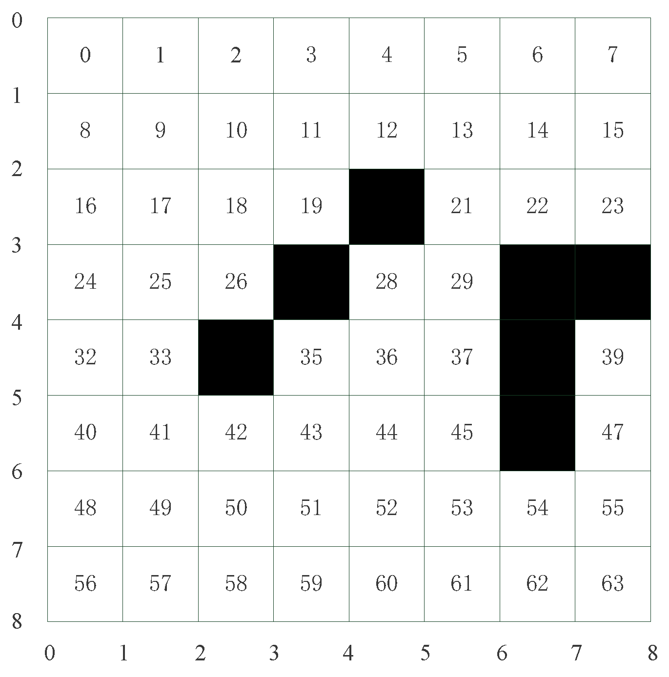
Figure 9.
Path diagram.

Figure 10.
The path image generated by the proposed algorithm.

Figure 11.
Location of remote wind farms. The green line represents mountains and the blue line represents rivers.
Figure 11.
Location of remote wind farms. The green line represents mountains and the blue line represents rivers.

Figure 12.
Solution of path planning.

Figure 13.
The results of path planning (Note: The yellow star represents the starting point).


Table 1.
Classification of literature review on path planning.
| Whether It Is a Hybrid Optimization Algorithm | Time | Main Research Work | Algorithm cATEGORY |
|---|---|---|---|
| No | 2019 | Liu et al. [5] used an ant colony algorithm to find the optimal path for inspection robots. Through simulation analysis, the ant colony algorithm reduces the time of shortest path searching, and increases the success rate of finding the optimal path. | Metaheuristic methods based on swarm |
| No | 2021 | Dong et al. [6] proposed a path planning method for an ultra-high voltage substation based on an ant colony optimization algorithm. Experimental results show that the algorithm could significantly improve the number of iterations. | Metaheuristic methods based on swarm |
| No | 2022 | In 2022, based on the improved biologically inspired neural network algorithm, Chen et al. [7] proposed a method of multi-mobile robot cooperative full-area coverage inspection. Simulation experiments verify the feasibility of the proposed multi-robot cooperative inspection scheme. | Metaheuristic methods based on biology |
| Yes | 2018 | He et al. [8] proposed an improved genetic simulated annealing algorithm. Compared with the optimization results of other path optimization algorithms, the proposed algorithm can obtain better travel path. | Metaheuristic methods based on biology and metaheuristic methods based on physics |
| Yes | 2019 | Yuan et al. [9] proposed a robot path-planning method based on simulated an annealing ant colony algorithm. Simulation results show that the algorithm can quickly plan the shortest and optimal inspection path. | Metaheuristic methods based on swarm and metaheuristic methods based on physics |
Table 2.
The number of legal paths varies with α.
| The Value of α | Number of Valid Paths n |
|---|---|
| 0 < α ≤ 0.03 | 0 < n ≤ 25 |
| 0.03 < α ≤ 0.05 | 30 < n ≤ 60 |
| 0.06 < α ≤ 0.08 | 80 < n < 100 |
| 0.09 < α ≤ 0.1 | 30 < n ≤ 50 |
| 0.11 < α ≤ 0.13 | 0 < n ≤ 10 |
| α > 0.13 | n = 0 |
Table 3.
The number of legal paths varies with β.
| The Value of β | Number of Valid Paths n |
|---|---|
| 0.001 < β ≤ 0.004 | 0 < n ≤ 15 |
| 0.005 < β ≤ 0.007 | 30 < n ≤ 70 |
| 0.008 < β ≤ 0.009 | 80 < n < 100 |
| 0.01 < β ≤ 0.02 | 30 < n ≤ 50 |
| 0.025 < β ≤ 0.04 | 0 < n ≤ 10 |
| 0.4 < β < 1 | n = 0 |
Table 4.
The number of legal paths varies with I0.
| The Value of I0 | Number of Valid Paths n |
|---|---|
| 0 < I0 ≤ 0.1 | 0 < n ≤ 15 |
| 0.1 < I0 ≤ 0.45 | 30 < n ≤ 75 |
| 0.45 < I0 ≤ 0.65 | 80 < n < 100 |
| 0.65 < I0 ≤ 0.75 | 30 < n ≤ 40 |
| 0.75 < I0 ≤ 0.8 | 0 < n ≤ 10 |
| 0.8 < I0 < 1 | n = 0 |
Table 5.
The number of legal paths varies with z (0).
| The Value of z (0) | Number of Valid Paths n |
|---|---|
| 0 < z (0) ≤ 0.3 | 0 < n ≤ 20 |
| 0.3 < z (0) ≤ 0.6 | 30 < n ≤ 50 |
| 0.6 < z (0) ≤ 0.8 | 80 < n < 100 |
| 0.8 < z (0) ≤ 0.9 | 45 < n ≤ 60 |
| 0.9 < z (0) ≤ 1 | 10 < n ≤ 30 |
| z (0) > 1 | n = 0 |
Table 6.
The number of legal paths varies with ε.
| The Value of ε | Number of Valid Paths n |
|---|---|
| 0 < ε ≤ 0.02 | 0 < n ≤ 30 |
| 0.02 < ε ≤ 0.04 | 40 < n ≤ 60 |
| 0.04 < ε ≤ 0.1 | 80 < n < 100 |
| 0.1 < ε ≤ 0.3 | 20 < n ≤ 30 |
| 0.3 < ε ≤ 0.5 | 10 < n ≤ 30 |
| ε > 0.5 | n = 0 |
Table 7.
The number of legal paths varies with Pc.
| The Value of Pc | Algorithm Optimization Performance |
|---|---|
| Pc < 0.4 | The speed of producing new individuals is slow |
| 0.4 ≤ Pc ≤ 0.99 | Obtain the optimal solution |
| Pc > 0.99 | The excellent pattern of population is easily destroyed |
Table 8.
The number of legal paths varies with Pm.
| The Value of Pm | Algorithm Optimization Performance |
|---|---|
| Pm < 0.01 | The ability to generate new individuals and inhibit premature phenomenon will be poor, which will affect the optimization performance of the algorithm. |
| 0.01 ≤ Pm ≤ 0.1 | Obtain the optimal solution |
| Pm > 0.1 | More new individuals can be generated, and many good patterns may be destroyed. The performance of the genetic algorithm is similar to that of a random search algorithm. |
Table 9.
Comparison of TSP City Travel Business Problem (75 cities).
| Operation Results | Best Results | Worst Result | Average Time | Average Optimization Rate | |
|---|---|---|---|---|---|
| Algorithm | |||||
| Grey Wolf Optimizer (GWO) | 9.5523 | 15.0516 | 56.619 s | 75.77% | |
| Firefly Algorithm (FA) | 7.1349 | 7.0772 | 159.6186 s | 31.29% | |
| Ant Colony Algorithm (ACA) | 5.6281 | 6.5804 | 107.784 s | 3.56% | |
| Genetic algorithm (GA) | 6.0926 | 6.9553 | 77.56 s | 12.11% | |
| TCNN | 6.124 | 8.9322 | 26.545 s | 12.69% | |
| proposed algorithm | 5.4345 | 6.2969 | 33.94 s | ≈0 | |
Note: k = 1, α = 0.07, β = 0.08, I0 = 0.65, z (0) = 0.8, ε = 0.05, W1 = 1, W2 = 1, Pc = 0.8, Pm = 0.07.
Table 10.
Comparison of TSP City Travel Business Problem (50 cities).
| Operation Results | Best Results | Worst Result | Average Time | Average Optimization Rate | |
|---|---|---|---|---|---|
| Algorithm | |||||
| Grey Wolf Optimizer (GWO) | 7.4258 | 8.4002 | 34.87 s | 35.99% | |
| Firefly Algorithm (FA) | 7.30 | 11.38 | 120.1204 s | 33.69% | |
| Ant Colony Algorithm (ACA) | 5.58 | 7.204 | 90.435 s | 2.19% | |
| Genetic algorithm (GA) | 5.7495 | 7.6771 | 64.608 s | 5.29% | |
| TCNN | 6.3398 | 7.153 | 21.7 s | 16.11% | |
| proposed algorithm | 5.5551 | 6.6146 | 28.94 s | 1.73% | |
Note: k = 1, α = 0.06, β = 0.08, I0 = 0.5, z (0) = 0.8, ε = 0.04, W1 = 1, W2 = 1, Pc = 0.65, Pm = 0.06.
Table 11.
Comparison of TSP City Travel Business Problem (100 cities).
| Operation Results | Best Results | Worst Result | Average Time | Average Optimization Rate | |
|---|---|---|---|---|---|
| Algorithm | |||||
| Grey Wolf Optimizer (GWO) | 17.6394 | 20.1142 | 76.809 s | 94.45% | |
| Firefly Algorithm (FA) | 14.65 | 27.03 | 2905.2109 s | 58.56% | |
| Ant Colony Algorithm (ACA) | 8.1728 | 16.0399 | 115.314 s | 2.44% | |
| Genetic algorithm (GA) | 8.6926 | 13.4465 | 99.79 s | 8.96% | |
| TCNN | 16.7864 | 19.0772 | 58.545 s | 72.8% | |
| proposed algorithm | 8.0345 | 10.2969 | 66.94 s | 0.71% | |
Note: k = 1, α = 0.08, β = 0.09, I0 = 0.65, z (0) = 0.8, ε = 0.08, W1 = 1, W2 = 1, Pc = 0.85, Pm = 0.09.
Table 12.
Comparison of TSP City Travel Business Problem (1000 cities).
| Operation Results | Best Results | Worst Result | Average Time | |
|---|---|---|---|---|
| Algorithm | ||||
| Grey Wolf Optimizer (GWO) | 421.7637 | 482.7657 | 690.728 s | |
| Firefly Algorithm (FA) | 328.65 | 437.03 | 11,322.9213 s | |
| Ant Colony Algorithm (ACA) | 265.5747 | 328.1901 | 915.314 s | |
| Genetic algorithm (GA) | 287.3142 | 326.639 | 444.598 s | |
| TCNN | 331.8651 | 349.1945 | 271.265 s | |
| proposed algorithm | 251.0795 | 279.5731 | 300.807 s | |
Note: k = 1, α = 0.08, β = 0.09, I0 = 0.65, z (0) = 0.8, ε = 0.1, W1 = 1, W2 = 1, Pc = 0.95, Pm = 0.1.
Table 13.
“Improvement” of different instances for 75 cities (The running time is 110s).
| % Improvement | Instance 1 | Instance 2 | Instance 3 | |
|---|---|---|---|---|
| Algorithm | ||||
| Grey Wolf Optimizer (GWO) | 52.696% | 54.47% | 57.64% | |
| Firefly Algorithm (FA) | 17.42% | 18.74% | 18.97% | |
| Ant Colony Algorithm (ACA) | 18.41% | 18.92% | 19.62% | |
| Genetic algorithm (GA) | 76.79% | 79.67% | 79.51% | |
| TCNN | 45.24% | 47.31% | 48.54% | |
| proposed algorithm | 79.65% | 80.99% | 82.35% | |
Table 14.
“Improvement” of different instances for 50 cities (The running time is 100s).
| % Improvement | Instance 1 | Instance 2 | Instance 3 | |
|---|---|---|---|---|
| Algorithm | ||||
| Grey Wolf Optimizer (GWO) | 55.40% | 57.89% | 47.71% | |
| Firefly Algorithm (FA) | 20.20% | 21.38% | 19.42% | |
| Ant Colony Algorithm (ACA) | 16.74% | 17.66% | 12.91% | |
| Genetic algorithm (GA) | 70.26% | 77.34% | 69.22% | |
| TCNN | 49.10% | 53.47% | 47.81% | |
| proposed algorithm | 77.09% | 79.03% | 76.45% | |
Table 15.
“Improvement” of different instances for 100 cities (The running time is 150 s).
| % Improvement | Instance 1 | Instance 2 | Instance 3 | |
|---|---|---|---|---|
| Algorithm | ||||
| Grey Wolf Optimizer (GWO) | 54.63% | 52.31% | 53.36% | |
| Firefly Algorithm (FA) | 19.58% | 16.52% | 17.34% | |
| Ant Colony Algorithm (ACA) | 20.16% | 17.99% | 18.67% | |
| Genetic algorithm (GA) | 81.48% | 78.75% | 79.26% | |
| TCNN | 53.45% | 50.78% | 51.48% | |
| proposed algorithm | 84.52% | 81.96% | 82.49% | |
Table 16.
The obtained algorithm comparison sequence values.
| Data Set | Proposed Algorithm | TCNN | GA | ACA | FA | GWO |
|---|---|---|---|---|---|---|
| D1 | 1 | 4 | 3 | 2 | 5 | 6 |
| D2 | 1 | 4 | 3 | 2 | 5 | 6 |
| D3 | 1 | 5 | 3 | 2 | 4 | 6 |
| D4 | 1 | 5 | 3 | 2 | 4 | 6 |
| The average sequence value | 1 | 4.5 | 3 | 2 | 4.5 | 6 |
Table 17.
Commonly used critical values for F-test.
| α = 0.1 | |||||||||
|---|---|---|---|---|---|---|---|---|---|
| Number of Data Sets N | Number of Algorithms k | ||||||||
| 2 | 3 | 4 | 5 | 6 | 7 | 8 | 9 | 10 | |
| 4 | 5538 | 3.463 | 2.813 | 2.480 | 2.273 | 2.130 | 2.023 | 1.940 | 1.874 |
| 5 | 4.545 | 3.113 | 2.606 | 2.333 | 2.158 | 2.035 | 1.943 | 1.870 | 1.811 |
| 8 | 3.589 | 2.726 | 2.365 | 2.157 | 2.019 | 1.919 | 1.843 | 1.782 | 1.733 |
| 10 | 3.360 | 2.624 | 2.299 | 2.108 | 1.980 | 1.886 | 1.814 | 1.757 | 1.710 |
| 15 | 3.102 | 2.503 | 2.219 | 2.048 | 1.931 | 1.845 | 1.779 | 1.726 | 1.682 |
| 20 | 2.990 | 2.448 | 2.182 | 2.020 | 1.909 | 1.826 | 1.762 | 1.711 | 1.668 |
Table 18.
qα values commonly used in Nemenyi test.
| α | Number of Algorithms k | ||||||||
|---|---|---|---|---|---|---|---|---|---|
| 2 | 3 | 4 | 5 | 6 | 7 | 8 | 9 | 10 | |
| 0.1 | 1.645 | 2.052 | 2.291 | 2.459 | 2.589 | 2.693 | 2.780 | 2.855 | 2.920 |
Table 19.
Comparison of wind farm path inspection results with detour obstacles.
| Operation Results | Best Results | Worst Result | Average Time | |
|---|---|---|---|---|
| Algorithm | ||||
| Grey Wolf Optimizer (GWO) | 7.1136 | 9.8808 | 18.219 s | |
| Firefly Algorithm (FA) | 5.2821 | 7.6176 | 86.3244 s | |
| Ant Colony Algorithm (ACA) | 4.7551 | 6.7835 | 30.939 s | |
| Genetic algorithm (GA) | 4.8965 | 5.0656 | 46.053 s | |
| TCNN | 4.9696 | 5.8965 | 23.354 s | |
| proposed algorithm | 4.5366 | 4.7446 | 22.09 s | |
Note: k = 1, α = 0.07, β = 0.08, I0 = 0.6, z (0) = 0.8, ε = 0.06, W1 = 1, W2 = 1, Pc = 0.85, Pm = 0.07.
Table 20.
Comparison of wind farm path inspection results with non-detour obstacles.
| Operation Results | Best Results | Worst Result | Average Time | |
|---|---|---|---|---|
| Algorithm | ||||
| Grey Wolf Optimizer (GWO) | 7.1525 | 8.9197 | 10.42 s | |
| Firefly Algorithm (FA) | 5.0085 | 7.6565 | 65.2261 s | |
| Ant Colony Algorithm (ACA) | 4.793 | 6.8224 | 22.939 s | |
| Genetic algorithm (GA) | 4.9354 | 5.1454 | 39.77 s | |
| TCNN | 5.321 | 6.4954 | 17.616 s | |
| proposed algorithm | 4.5755 | 4.7835 | 21.768 s | |
Note: k = 1, α = 0.07, β = 0.08, I0 = 0.55, z (0) = 0.8, ε = 0.06, W1 = 1, W2 = 1, Pc = 0.8, Pm = 0.07.
Publisher’s Note: MDPI stays neutral with regard to jurisdictional claims in published maps and institutional affiliations. |
© 2022 by the authors. Licensee MDPI, Basel, Switzerland. This article is an open access article distributed under the terms and conditions of the Creative Commons Attribution (CC BY) license (https://creativecommons.org/licenses/by/4.0/).
Share and Cite
MDPI and ACS Style
Chen, L.; Hu, Z.; Zhang, F.; Guo, Z.; Jiang, K.; Pan, C.; Ding, W. Remote Wind Farm Path Planning for Patrol Robot Based on the Hybrid Optimization Algorithm. Processes 2022, 10, 2101. https://doi.org/10.3390/pr10102101
AMA Style
Chen L, Hu Z, Zhang F, Guo Z, Jiang K, Pan C, Ding W. Remote Wind Farm Path Planning for Patrol Robot Based on the Hybrid Optimization Algorithm. Processes. 2022; 10(10):2101. https://doi.org/10.3390/pr10102101
Chicago/Turabian StyleChen, Luobing, Zhiqiang Hu, Fangfang Zhang, Zhongjin Guo, Kun Jiang, Changchun Pan, and Wei Ding. 2022. "Remote Wind Farm Path Planning for Patrol Robot Based on the Hybrid Optimization Algorithm" Processes 10, no. 10: 2101. https://doi.org/10.3390/pr10102101
Note that from the first issue of 2016, this journal uses article numbers instead of page numbers. See further details here.