A New Modified Exponent Power Alpha Family of Distributions with Applications in Reliability Engineering

Abstract

Probability distributions perform a very significant role in the field of applied sciences, particularly in the field of reliability engineering. Engineering data sets are either negatively or positively skewed and/or symmetrical. Therefore, a flexible distribution is required that can handle such data sets. In this paper, we propose a new family of lifetime distributions to model the aforementioned data sets. This proposed family is known as a “New Modified Exponent Power Alpha Family of distributions” or in short NMEPA. The proposed family is obtained by applying the well-known T-X approach together with the exponential distribution. A three-parameter-specific sub-model of the proposed method termed a “new Modified Exponent Power Alpha Weibull distribution” (NMEPA-Wei for short), is discussed in detail. The various mathematical properties including hazard rate function, ordinary moments, moment generating function, and order statistics are also discussed. In addition, we adopted the method of maximum likelihood estimation (MLE) for estimating the unknown model parameters. A brief Monte Carlo simulation study is conducted to evaluate the performance of the MLE based on bias and mean square errors. A comprehensive study is also provided to assess the proposed family of distributions by analyzing two real-life data sets from reliability engineering. The analytical goodness of fit measures of the proposed distribution are compared with well-known distributions including (i) APT-Wei (alpha power transformed Weibull), (ii) Ex-Wei (exponentiated-Weibull), (iii) classical two-parameter Weibull, (iv) Mod-Wei (modified Weibull), and (v) Kumar-Wei (Kumaraswamy–Weibull) distributions. The proposed class of distributions is expected to produce many more new distributions for fitting monotonic and non-monotonic data in the field of reliability analysis and survival analysis.

1. Introduction

In the field of reliability engineering as well as other related fields, the modeling of lifetime events is of great importance. Generally, numerous probability distributions are available to model such types of lifetime data that are uncertain and complex in nature. However, in many cases, these probability distributions are suitable to model lifetime data.

In the literature, the exponential and Rayleigh distributions are the most popular and widely used distributions in lifetime analysis. However, when the lifetime data sets are complex then these probability distributions are not suitable to represent data accurately. For example, the Exponentiated distribution is concerned with describing data that have a constant failure rate function; on the other hand, the Ray distribution is used to model data that possess an increasing failure rate function. Similarly, the Weibull (Wei) distribution is one of the important lifetime distributions, which has both the characteristic of Exponentiated and Rayleigh distributions and has widely been used in the field of reliability engineering and in other research areas; see, Lee et al. [1]. Although the Wei distribution is widely used in many fields, it is confined to the structure of its HF (hazard function) only increasing, decreasing, and constant. Generally, many significant issues require a flexible range of HF; for instance, human mortality and life cycles of electronic machines and components lifetime events possess a bathtub and unimodal-shaped HF. To overcome these difficulties, we need a more flexible version of the Wei distribution to model reliability data adequately. In this regard, researchers’ efforts have been devoted to deriving new models or families of statistical models to provide a better description of the problem under consideration. Such models have been constructed by inserting one or more new additional parameters to the baseline models to obtain new models that are analytically more flexible and provide better fits to the lifetime events than the other adapted models; see a new modified alpha power (MPA) family of distributions proposed by Hussein et al. [2]; the new exponential-X (NExp-X) family proposed by Shah et al. [3]; the Z-family introduced by Ahmad et al. [4]; the new generalized-X (NG-X) family proposed by Wang et al. [5]; the transmuted alpha power-G (TAP-G) family presented by Eghwerido et al. [6]; the unit extended Weibull (UEx-Wei) families proposed by Guerra et al. [7]; and a new lifetime-X (NLT-X) family introduced by Mohammed et al. [8].

Mudholkar and Srivastava [9] proposed a simple Exponentiated method by inserting an extra parameter into the family of distributions. The CDF (cumulative distribution function) is given by

$$K\left(y;\alpha ,\Delta \right)={\left[G\left(y;\Delta \right)\right]}^{\alpha },\hspace{1em}\hspace{1em}\alpha >0,y\in ℝ,$$

(1)

where $G\left(y;\Delta \right)$ is the CDF of any baseline distributions depending on the parameter vector $\Delta$. Cordeiro and de Castro [10] developed a method to incorporate an additional parameter to the baseline distribution, which has the following form,

$$K\left(y;\alpha ,\beta ,\Delta \right)=1-{\left[1-G{\left(y;\Delta \right)}^{\alpha }\right]}^{\beta },\hspace{1em}\alpha ,\beta >0, y\in ℝ,$$

(2)

using Equation (2), Cordiero and de Castro [10] defined four parameters of Kumaraswamy Wei distribution. Moreover, using Equation (2), different researchers extended the classical Wei distribution; see for example ([11,12,13,14]).

Similarly, Marshal and Olkin [15] introduced Marshall–Olkin generated (MO-G) family using the following CDF

$$K\left(y;\alpha ,\Delta \right)=\frac{G\left(y;\Delta \right)}{1-(1-\alpha )\left[1-G\left(y;\Delta \right)\right]},\alpha ,\beta ,\Delta >0,y\in ℝ,$$

(3)

using Equation (3), Marshal and Olkin [15] derived two special sub-models, namely, the Marshal–Olkin Exponential (MO-Exp) and Marshal–Olkin Wei (MO-Wei) distributions. Later on, using Equation (3), several probability distributions were proposed in the literature; for instance, see the work given in ([16,17,18]).

Recently, in this regard, Khan et al. [19] proposed an exponentiated odd generalized exponential (OGE2-G) family of distribution using the following CDF

$$K\left(y;\alpha ,\delta ,\Delta \right)={\left(1-e^{-\frac{1-\overline{G}{(y;\Delta )}^{\alpha }}{\overline{G}{(y;\Delta )}^{\alpha }}}\right)}^{\delta },\hspace{1em}\hspace{1em}\alpha ,\delta ,\Delta >0,y\in ℝ,$$

(4)

Using Equation (4), Khan et al. [19] also derived a four-parameter exponentiated odd generalized exponential Fréchet (OGE2Fr) distribution.

In this manuscript, we propose a new flexible class family of distributions by implementing the method of the T-X approach together with exponential distribution having density function $m\left(t\right)=e^{-t}$. The new proposed class is called an NMEPA family of distributions, which capitalizes on the weaknesses of the available distributions in the literature. The main motivations for using the NMEPA method in practice are the following: (i) the method has not been proposed/used so far; (ii) to improve the existing distributions, and numerous new distributions can also be proposed for data modeling in the different phenomenon; (iii) to generalize the existing distributions with a closed form of their distribution functions; (iv) to provide the best fit to real-world data as compared the other distributions having the fever, and same or higher number of parameters; and (v) to provide the best fit to the considered data sets, describing the reliability in engineering. In fact, we conclude empirically that the new modification of the Wei distribution offers the best fit to the considered data sets in comparison to the two, three, and four-parameter competing distributions.

2. The Proposed NMEPA Family

In this section, we introduce a new modified method to derive a new lifetime distribution. The proposed method is introduced by combining the exponential model having PDF (probability density function) $m\left(t\right)=e^{-t}$ with the T-X family proposed by Alzaatreh et al. [20].

Consider a random variable, say T be a baseline random variable with PDF $m\left(t\right)$, where $T\in$ [$a_1$, $a_2$] for $-\infty \le a_1<a_2\le \infty$. Let $y$ be a random variable with CDF (cumulative distribution function) $G\left(y;\Delta \right)$ depending on the parameter vector $\Delta$. In addition, suppose that $F\left[G\left(y;\Delta \right)\right]$ be a function of CDF of $y$, satisfying the following three conditions,

• $F\left[U\left(y;\Delta \right)\right]\in \left[a_1,a_2\right]$,

• $F\left[G\left(y;\Delta \right)\right]$ is differentiable and monotonically increasing,

• $F\left[G\left(y;\Delta \right)\right]\to a_1$ as $y\to -\infty$ and $F\left[G\left(y;\Delta \right)\right]\to a_2$ as $y\to \infty$.

Then, according to Alzaatreh et al. [20], the CDF of the T-X family is defined by

$$K_{T-X}\left(y\right)=K\left(y;\Delta \right)={\displaystyle {\int }_{a_1}^{F[G\left(y;\Delta \right) ]}m\left(t\right)dt,}$$

(5)

where $F\left[G(y;\Delta )\right]$ satisfies certain conditions given above. The PDF of T-X distribution, corresponding to Equation (5) is given by;

$$k_{T-X}\left(y\right)=k\left(y;\Delta \right)=m\left(F\left[G\left(y;\Delta \right)\right]\right)\frac{d}{dy}F\left[G\left(y;\Delta \right)\right]$$

(6)

Now, by using $m\left(t\right)=e^{-t}$ and setting $F\left[G(y;\Delta )\right]=-\log \left(1-\frac{G(y;\Delta )e^{\left(1-{\left(\overline{\alpha }\right)}^2\right)}}{e^{\left(1-{\left(1-\alpha G(y;\Delta )\right)}^2\right)}}\right)$ in Equation (5), we obtain the CDF $K\left(y;\alpha ,\Delta \right)$ of the NMEPA family of distributions, given by

$$K\left(y;\alpha ,\Delta \right)=\frac{e^{\left(1-{\left(\overline{\alpha }\right)}^2\right)}G(y;\Delta )}{e^{\left(1-{\left(1-\alpha G(y;\Delta )\right)}^2\right)}},\alpha >0, y\in ℝ,$$

(7)

the CDF may also be written in the following form,

$$K\left(y;\alpha ,\Delta \right)=\frac{G(y;\Delta )}{\exp \left({\left(\overline{\alpha }\right)}^2-{\left(1-\alpha G(y;\Delta )\right)}^2\right)},\hspace{1em}\hspace{1em}\alpha >0, y\in ℝ,$$

where $\overline{\alpha }=1-\alpha$, and $G\left(y;\Delta \right)$ is the CDF of the baseline distribution with parameters vector $\Delta$.

The PDF $k\left(y;\alpha ,\Delta \right)$ of the NMEPA family associated with Equation (7) is given by

$$k\left(y;\alpha ,\Delta \right)=\frac{g(y;\Delta )\left[1-2\alpha G(y;\Delta )\left(1-\alpha G(y;\Delta )\right)\right]}{{\mathrm{e}}^{\left({\left(\overline{\alpha }\right)}^2-{\left(1-\alpha G(y;\Delta )\right)}^2\right)}},\alpha >0, y\in ℝ,$$

(8)

where $\frac{d}{dy}G\left(y;\Delta \right)=g\left(y;\Delta \right)$.

Corresponding to Equations (7) and (8), the SF (survival function) and HF (hazard function) are given as follows:

$$S\left(y;\alpha ,\Delta \right)=1-\frac{G(y;\Delta )}{{\mathrm{e}}^{\left({\left(\overline{\alpha }\right)}^2-{\left(1-\alpha G(y;\Delta )\right)}^2\right)}},\hspace{1em}\alpha >0, y\in ℝ,$$

(9)

and

$$h\left(y;\alpha ,\Delta \right)=\frac{g(y;\Delta )\left[1-2\alpha G(y;\Delta )\left(1-\alpha G(y;\Delta )\right)\right]}{{\mathrm{e}}^{\left({\left(\overline{\alpha }\right)}^2-{\left(1-\alpha G(y;\Delta )\right)}^2\right)}-G(y;\Delta )}$$

(10)

In this article, using Equation (7) we propose a new generalized/extended version of the Wei distribution, namely, an NMEPA-Wei (new modified exponent power alpha Wei) distribution. The NMEPA-Wei model is compared with five other well-known probability distributions including (a) three-parameter APT-Wei (alpha power transformed Wei) [21], (b) Ex-Wei (exponentiated Wei), [9], (c) two-parameter classical Wei [22], (d) Sarhan and Zaindin Mod-Wei (Modified Wei) [23], and (e) four-parameter Ku-Wei (Kumaraswamy Wei) distributions [10], by analyzing two real data sets in the field of reliability engineering. The following Section 2.1, offers the CDF, PDF, SF, HF, and CHF (cumulative hazard function) of the NMEPA-Wei distribution. Furthermore, different PDF and HF behaviors are also presented graphically in the same section. The rest of the work in this study is organized as follows: In Section 3, the statistical properties of the proposed NMEPA family of distributions are also discussed. The method of MLE for the proposed distribution is described in Section 4. In Section 4.1, a brief Monte Carlo simulation study is carried out. The comprehensive analyses using two engineering data sets are discussed in Section 5. Finally, some concluding remarks are given in Section 6.

2.1. The NMEP-Wei Distribution

Consider the CDF $G(y;\Delta )$ and PDF $g(y;\Delta )$ of the classical two-parameter $\left(\gamma >0,\theta >0\right)$ Wei distribution given by

$$G(y;\Delta )=1-e^{-\gamma x^{\theta }},\hspace{1em}y\ge 0,$$

(11)

and

$$g(y;\Delta )=\gamma \theta x^{\theta -1}{e}^{-\gamma x^{\theta }},\hspace{1em}y>0,$$

(12)

where $\Delta =\left(\gamma ,\theta \right)$.

Using Equation (11) in Equation (7) yields the CDF $K\left(y;\alpha ,\Delta \right)$ of the NMEPA-Wei distribution, which is given by

$$K\left(y;\alpha ,\Delta \right)=\frac{e^{\left(1-{\left(\overline{\alpha }\right)}^2\right)}(1-e^{-\gamma y^{\theta }})}{e^{\left(1-{\left(1-\alpha (1-e^{-\gamma y^{\theta }})\right)}^2\right)}},\hspace{1em}\hspace{1em}y\ge 0,\alpha ,\gamma ,\theta >0,$$

(13)

with PDF

$$k\left(y;\alpha ,\Delta \right)=\frac{\gamma \theta x^{\theta -1}{e}^{-\gamma y^{\theta }}\left[1-2\alpha (1-e^{-\gamma y^{\theta }})\left(1-\alpha (1-e^{-\gamma y^{\theta }})\right)\right]}{{\mathrm{e}}^{\left({\left(\overline{\alpha }\right)}^2-{\left(1-\alpha (1-e^{-\gamma y^{\theta }})\right)}^2\right)}}, y>0$$

(14)

Different plots of the PDF $k\left(y;\alpha ,\Delta \right)$ of the NMEPA-Wei distribution are presented in Figure 1a,b for different values of the parameters $\alpha ,\gamma$ and $\theta$. From Figure 1a,b, we can see different PDF patterns including bio-modal, left-skewed, right-skewed, and symmetrical curves.

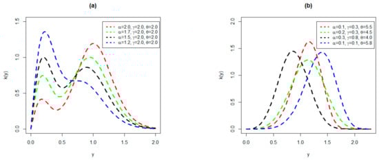
Figure 1. Plots of (a) bi-modal, and (b) left-skewed, right-skewed, and symmetrical PDF $k\left(y;\alpha ,\Delta \right)$ of the proposed NMEPA-Wei distribution.

Furthermore, the SF $S\left(y;\alpha ,\Delta \right)$, HF $h\left(y;\alpha ,\Delta \right)$, and CHF (cumulative hazard function) $H\left(y;\alpha ,\Delta \right)$ of the NMEPA-Wei distribution are given by

$$S\left(y;\alpha ,\Delta \right)=1-\frac{\left(1-e^{\gamma y^{\theta }}\right)}{{\mathrm{e}}^{\left({\left(\overline{\alpha }\right)}^2-{\left(1-\alpha (1-e^{\gamma y^{\theta }})\right)}^2\right)}},\hspace{1em}y>0,$$

(15)

$$h\left(y;\alpha ,\Delta \right)=\frac{\gamma \theta x^{\theta -1}{e}^{-\gamma y^{\theta }}\left[1-2\alpha (1-e^{-\gamma y^{\theta }})\left(1-\alpha (1-e^{-\gamma y^{\theta }})\right)\right]}{{\mathrm{e}}^{\left({\left(\overline{\alpha }\right)}^2-{\left(1-\alpha (1-e^{-\gamma y^{\theta }})\right)}^2\right)}-(1-e^{-\gamma y^{\theta }})},y>0,$$

(16)

and

$$H\left(y;\alpha ,\Delta \right)=\log \left(1-\frac{\left(1-e^{\gamma y^{\theta }}\right)}{{\mathrm{e}}^{\left({\left(\overline{\alpha }\right)}^2-{\left(1-\alpha (1-e^{\gamma y^{\theta }})\right)}^2\right)}}\right),\hspace{1em}y>0,$$

(17)

respectively.

Here, different plots of the HF $h\left(y;\alpha ,\Delta \right)$ of the NMEP-Wei distribution are presented in Figure 2a,b. From Figure 2a, we can see increasing and decreasing HF $h\left(y;\alpha ,\Delta \right)$, while in Figure 2b, we can see uni-modal HF $h\left(y;\alpha ,\Delta \right)$. Similarly, from Figure 3, we can see bathtub HF $h\left(y;\alpha ,\Delta \right)$ of the NMEPA-Wei distribution.

Figure 2. Plots of (a) increasing, and decreasing, and (b) unimodal HF $h\left(y;\alpha ,\Delta \right)$ of the NMEPA-Wei distribution.

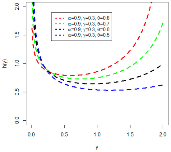
Figure 3. Plots of different bathtub shapes of HF $h\left(y;\alpha ,\Delta \right)$ of the proposed NMEPA-Wei distribution.

3. Statistical Properties of NMEPA Family

In this section, various mathematical properties of the proposed family of distributions such as QF (quantile function), and ordinary moments that can further be used to obtain some important characteristics of the model are discussed. In addition to these properties, the MGF (moment generating function) and OS (order statistics) are also derived.

3.1. Quantile Function

The QF also called IDF (inverse distribution function) is an important statistical characteristic used to generate random numbers (RNs). The QF of the NMEPA distribution is a function $Q\left(u;\Delta \right)$ that satisfies the following nonlinear equation

$$Q\left(K\left(u;\Delta \right);\Delta \right)=u$$

where $u\in \left(0,1\right)$. By using Equation (7) and after some algebraic manipulation the QF is derived as

$$Q\left(K\left(u;\Delta \right);\Delta \right)=K^{-1}\left(u\right)=G^{-1}\left(u\right)$$

(18)

where u is the solution of the nonlinear equation $\log \left(u\right)-{\left(1-\alpha G\left(y;\Delta \right)\right)}^2+{\overline{\alpha }}^2-\log G\left(y;\Delta \right)$. The expression (18) can also be used to measure the effect of parameters on Skewness and Kurtosis. Hence, the formulas for Skewness and Kurtosis are the following expression

$$\mathrm{Skewness}=\frac{Q\left(1/4\right)-2Q\left(1/2\right)+Q\left(3/4\right)}{Q\left(3/4\right)-Q\left(1/4\right)},$$

and

$$\mathrm{Kurtosis}=\frac{Q\left(7/8\right)-\left[Q\left(5/8\right)+Q\left(1/8\right)\right]+Q\left(3/8\right)}{Q\left(6/8\right)-Q\left(2/8\right)}.$$

The mean, variance, skewness, and kurtosis for $\gamma =$ 1, and different values of $\alpha$ and $\theta$, of the NMEPA-Wei distribution, are sketched in Figure 4.

Figure 4. Different plots of (a) mean, (b) variance, (c) skewness, and (d) kurtosis of the NMEPA-Wei model.

3.2. rth Moments

The rth moment is an important and useful statistical tool to obtain certain characteristics and features of a model. These characteristics are known as (i) central tendency, which deals with the mean point of distribution; (ii) dispersion, which measures the variance of a model; (iii) skewness, which describes the tail behavior of the model; and (iv) kurtosis, which helps in studying the peakedness of the distribution. Let $y$ be a random variable that follows the NMEPA-Wei distribution, then its rth moment can be expressed as follows,

$${\mu }_r^{\prime }={\displaystyle {\mathrm{\int }}_{-\infty }^{\infty }\stackrel{r}{y}} k\left(y;\alpha ,\Delta \right)dy.$$

(19)

Using Equation (8) in Equation (18), we have

$${\mu }_r^{\prime }={\displaystyle {\mathrm{\int }}_{-\infty }^{\infty }\stackrel{r}{y}}\frac{g(y;\Delta )\left[1-2\alpha G(y;\Delta )\left(1-\alpha G(y;\Delta )\right)\right]}{{\mathrm{e}}^{\left({\left(\overline{\alpha }\right)}^2-{\left(1-\alpha G(y;\Delta )\right)}^2\right)}}dy,$$

(20)

Using the following series

$${\mathrm{e}}^y={\displaystyle \sum _{i=0}^{\infty }\frac{y^i}{i!}}$$

(21)

and using $y=\left({\left(\overline{\alpha }\right)}^2-{\left(1-\alpha G(y;\Delta )\right)}^2\right)$ in Equation (20), we obtain

$${\mathrm{e}}^{\left({\left(\overline{\alpha }\right)}^2-{\left(1-\alpha G(y;\Delta )\right)}^2\right)}={\displaystyle \sum _{i=0}^{\infty }\frac{{\left({\left(\overline{\alpha }\right)}^2-{\left(1-\alpha G(y;\Delta )\right)}^2\right)}^i}{i!}}$$

$${\mathrm{e}}^{\left({\left(\overline{\alpha }\right)}^2-{\left(1-\alpha G(y;\Delta )\right)}^2\right)}={\displaystyle \sum _{i=0}^{\infty }\frac{{\left(\overline{\alpha }\right)}^2{}^i}{i!}}{\left(1-\frac{{\left(1-\alpha G(y;\Delta )\right)}^2}{{\left(\overline{\alpha }\right)}^2}\right)}^i$$

(22)

In addition, using the following series representation for Equation (22)

$${\left(1-y\right)}^i={\displaystyle \sum _{j=0}^i{\left(-1\right)}^j}\left(\begin{array}{c}v\\ j\end{array}\right)y^j$$

(23)

Using $y=\frac{{\left(1-\alpha G(y;\Delta )\right)}^2}{{\left(\overline{\alpha }\right)}^2}$ in Equation (23), we obtain

$${\mathrm{e}}^{\left({\left(\overline{\alpha }\right)}^2-{\left(1-\alpha G(y;\Delta )\right)}^2\right)}={\displaystyle \sum _{i=0}^{\infty }{\displaystyle \sum _{j=0}^i\frac{{\left(\overline{\alpha }\right)}^2{}^{i-2j}}{i!}{\left(-1\right)}^j\left(\begin{array}{c}i\\ j\end{array}\right)}{\left(1-\alpha G(y;\Delta )\right)}^{2j}}$$

(24)

again using series representation in Equation (23), and replacing $y=\alpha U(y;\Delta )$, we obtain

$${\mathrm{e}}^{\left({\left(\overline{\alpha }\right)}^2-{\left(1-\alpha G(y;\Delta )\right)}^2\right)}={\displaystyle \sum _{i=0}^{\infty }{\displaystyle \sum _{j=0}^i{\displaystyle \sum _{l=0}^{2j}\frac{{\alpha }^l{\left(\overline{\alpha }\right)}^2{}^{i-2j}}{i!}{\left(-1\right)}^{j+l}\left(\begin{array}{c}i\\ j\end{array}\right)}\left(\begin{array}{c}2j\\ l\end{array}\right)G{(y;\Delta )}^l}}$$

(25)

By inserting Equation (25) in Equation (20), we obtain the following expression

$${\mu }_r^{\prime }=\frac{1}{{\eta }_{i,j,l}}\left({\mathsf{\Psi }}_{r,-l}-2\alpha {\mathsf{\Psi }}_{r,1-l}-2{\alpha }^2{\mathsf{\Psi }}_{r,2-l}\right)$$

(26)

where ${\eta }_{i,j,l}={\displaystyle \sum _{i=0}^{\infty }{\displaystyle \sum _{j=0}^i{\displaystyle \sum _{l=0}^{2j}\frac{{\alpha }^l{\left(\overline{\alpha }\right)}^2{}^{i-2j}}{i!}{\left(-1\right)}^{j+l}\left(\begin{array}{c}i\\ j\end{array}\right)}\left(\begin{array}{c}2j\\ l\end{array}\right)}}$, from Equation (26), we have

$${\mu }_r^{\prime }=\frac{1}{{\eta }_{i,j,l}}\left({\mathsf{\Psi }}_{r,-l}-2\alpha \left({\mathsf{\Psi }}_{r,1-l}+\alpha {\mathsf{\Psi }}_{r,2-l}\right)\right)$$

(27)

where ${\mathsf{\Psi }}_{r,-l}={\displaystyle \underset{-\infty }{\overset{\infty }{\int }}{y}^{r}k\left(y;\alpha ,\Delta \right)K{\left(y;\alpha ,\Delta \right)}^{-l}dy}$, ${\mathsf{\Psi }}_{r,1-l}={\displaystyle \underset{-\infty }{\overset{\infty }{\int }}{y}^{r}k\left(y;\alpha ,\Delta \right)K{\left(y;\alpha ,\Delta \right)}^{1-l}dy}$, and ${\mathsf{\Psi }}_{r,2-l}={\displaystyle \underset{-\infty }{\overset{\infty }{\int }}{y}^{r}k\left(y;\alpha ,\Delta \right)K{\left(y;\alpha ,\Delta \right)}^{2-l}dy}$.

Furthermore, the MGF (moment generating function), say $M_y\left(t\right)$ of the NMEPA family of distribution, is derived as follows

$$M_y\left(t\right)={\displaystyle \underset{-\infty }{\overset{\infty }{\int }}{e}^{ty}k\left(y;\alpha ,\Delta \right)dy}$$

$$M_y\left(t\right)={\displaystyle \sum _{r=0}^{\infty }\frac{t^r}{r!}}{\displaystyle \underset{0}{\overset{\infty }{\int }}{y}^{r}k\left(y;\alpha ,\Delta \right)dy}$$

$$M_y\left(t\right)={\displaystyle \sum _{r=0}^{\infty }\frac{t^r}{r!}} {\mu }_r^{\prime }$$

(28)

By using Equation (27) in Equation (28), we can easily obtain the MGF of the NMEPA family of distributions.

3.3. Order Statistics

In distribution theory, order statistics has great significance and it makes its appearance in reliability analysis, problems of estimation theory, and life testing in different ways. It can characterize the lifetimes of elements or components of a reliability system.

Let $y_1, {\mathrm{y}}_2,\dots , {\mathrm{y}}_k$ be a random sample of $q$ observations chosen from the NMEPA family of distributions with CDF and PDF given by (7) and (8), respectively. Then, the density function of $w_{r:q}$ is given by

$$W_{r:q}\left(y\right)=\frac{1}{B\left(r,q-r+1\right)}k\left(y;\alpha ,\Delta \right){\left[K\left(y;\alpha ,\Delta \right)\right]}^{r-1}{\left[1-K\left(y;\alpha ,\Delta \right)\right]}^{q-r}.$$

(29)

We express the 1st order statistic as $y_{1:q}=\min \left(y_1, {\mathrm{y}}_2,\dots , {\mathrm{y}}_q\right)$ and the qth order statistic as $y_{q:q}=\max \left(y_1, {\mathrm{y}}_2,\dots , {\mathrm{y}}_q\right).$ Since $0<K\left(y;\alpha ,\Delta \right)<1$ for $y>0$. We utilize the binomial expansion of ${\left[1-K\left(y;\alpha ,\Delta \right)\right]}^{q-r}$ as follows:

$${\left[1-K\left(y;\alpha ,\Delta \right)\right]}^{q-r}={\displaystyle \sum _{i=0}^{q-r}{\left(-1\right)}^i}{\left[{\left[1-K\left(y;\alpha ,\Delta \right)\right]}^{q-r}\right]}^i.$$

(30)

Using Equation (30) in Equation (29), we obtain

$$w_{r:q}\left(y\right)=\frac{k\left(y;\alpha ,\Delta \right)}{B\left(r,q-r+1\right)}{\displaystyle \sum _{i=0}^{k-r}{\left(-1\right)}^i}{\left[K\left(y;\alpha ,\Delta \right)\right]}^{r+i-1}.$$

(31)

Using Equations (7) and (8), in Equation (31), we obtain the DF (density function) of $w_{r:q}$.

4. Estimation of Parameters and Monte Carlo Simulation

This section provides a detailed description of the maximum likelihood estimation implemented for estimating unknown parameters of the proposed NMEPA family of distribution. Furthermore, we conduct a comprehensive Monte Carlo simulation study for assessing the performance of these estimators. The same section also provides an assessment of the efficacy of the proposed method in modeling reliability engineering problems.

4.1. Maximum Likelihood Estimation

Several methods for estimating the parameters have been introduced in the literature. MLE is one of the most frequently used methods. This method furnishes estimators with several important properties and can be used in the construction of confidence intervals as well as other tests for checking statistical significance. For further details about MLEs, see [24]. This sub-section provides a discussion on the MLEs approach for estimating the parameters of the NMEPA family of distributions.

Suppose $y_1,y_2,\dots ,y_n$ are the observed values from the PDF given in Equation (8). Then, the LLF (Log-likelihood function) corresponding to Equation (8) is

$$\begin{array}{l}L\left(y;\alpha ,\Delta \right)={\displaystyle \sum _{i=1}^{\infty }\log g\left(y_i;\Delta \right)}-n\log (2)-n\log (\alpha )-{\displaystyle \sum _{i=1}^{\infty }\log \left\{1-\alpha G(y_i;\Delta )\right\}}\\ \hspace{1em}\hspace{1em}-\left({\left(\overline{\alpha }\right)}^2-{\left(1-\alpha G(y_i;\Delta )\right)}^2\right)\end{array}$$

(32)

Generally, the LLF (log-likelihood function) can be maximized either directly by using the R package (Adequacy Model), Ox program (subroutine Max BFGS), or SAS (PROC NLMIXED) (for further details, see Doornik, [25]), or by solving the nonlinear log-likelihood equations. Here, we obtain the partial derivative of Equation (32), on behalf of parameters and it is given as follows:

$$\begin{array}{l}\frac{\partial L\left(y;\alpha ,\Delta \right)}{\partial \alpha }={\displaystyle \sum _{i=1}^{\infty }G(y_i;\alpha ,\Delta )/\left(1-\alpha G(y_i;\Delta )\right)}+2\left(\overline{\alpha }\right)\\ \hspace{1em}\hspace{1em}-\frac{n}{\alpha }+2{\left(1-\alpha G(y_i;\Delta )\right)}^{2}G(y_i;\Delta ),\end{array}$$

(33)

and

$$\begin{array}{l}\frac{\partial L\left(y;\alpha ,\Delta \right)}{\partial \Delta }={\displaystyle \sum _{i=1}^{\infty }\frac{\partial g\left(y_i;\Delta \right)/\partial \Delta }{g\left(y_i;\Delta \right)}}+\alpha {\displaystyle \sum _{i=1}^{\infty }\frac{\partial G(y_i;\Delta )/\partial \Delta }{\left(1-\alpha G(y_i;\Delta )\right)}}\\ \hspace{1em}\hspace{1em}\hspace{1em}\hspace{1em} +2\alpha \left(1-\alpha G(y_i;\Delta )\right)\partial G(y_i;\Delta )/\partial \Delta .\end{array}$$

(34)

Equating Equation (33) $\frac{\partial L\left(y;\alpha ,\Delta \right)}{\partial \alpha }$ and Equation (34) $\frac{\partial L\left(y;\alpha ,\Delta \right)}{\partial \Delta }$ to zero, and solving simultaneously, yield the MLEs of $\left(\hat{\alpha },\hat{\Delta }\right)$.

4.2. Simulation Study

In this sub-section, a simulation is performed to study the behavior of $\hat{\alpha }MLE$, and $\hat{\Delta }MLE$ of the NMEPA-Wei distribution. The random numbers are successfully generated from PDF $k\left(y;\alpha ,\Delta \right)$ by using the inverse CDF approach. We are assumed to have three sets (Set 1, Set 2, and Set 3) of parameter combination values, given by (i) Set 1: $\alpha =$ 1.4, $\gamma =$ 1.0, $\theta =$ 1.6, (ii) Set 2: $\alpha =$ 2.4, $\gamma =$ 1.7, $\theta =$ 1.5, and (iii) Set 3: $\alpha =$ 0.5, $\gamma =$ 1.2, $\theta =$ 1.6.

To evaluate the performance of the $\hat{\alpha }MLE$, and $\hat{\Delta }MLE$, two statistical measures (i) MSE (mean square error), and (ii) Bias are considered. The formula of mean square error (MSEs) and bias (Bias) of the parameters are, respectively, computed as

$$MES(\hat{\alpha })={{\displaystyle \sum _{i=1}^{1000}\left({\hat{\alpha }}_i-\alpha \right)}}^2$$

and

$$Bias(\hat{\alpha })={\displaystyle \sum _{i=1}^{1000}\left({\hat{\alpha }}_i-\alpha \right)}$$

The above process is also repeated for $\Delta$.

Simulation results on estimated parameters in terms of MSEs and Bias values are reported in Table 1, while graphically the results are displayed in Figure 5, Figure 6, Figure 7, Figure 8, Figure 9 and Figure 10.

Table 1. Simulation results for NMEPA-Wei distribution of MLEs, MSEs, and Biases for Set 1, Set 2, and Set 3.

		$\mathit{S}\mathit{e}\mathit{t}1:\mathit{\alpha }=1.4, \mathit{\gamma }=1.0, \mathit{\theta }=1.6$			$\mathit{S}\mathit{e}\mathit{t}2:\mathit{\alpha }=2.4, \mathit{\gamma }=1.7, \mathit{\theta }=1.5$			$\mathit{S}\mathit{e}\mathit{t}3:\mathit{\alpha }=0.5, \mathit{\gamma }=1.2, \mathit{\theta }=1.6$
n	par	MLE	MSE	Bias	MLE	MSE	Bias	MLE	MSE	Bias
25	$\hat{\alpha }$	1.41090	0.07820	0.01090	2.67742	0.66393	0.02774	0.56813	0.20871	0.06813
	$\hat{\gamma }$	1.05926	0.11310	0.05926	1.85403	0.42708	0.01540	1.62178	0.54727	0.42178
	$\hat{\theta }$	1.05926	0.09874	0.03332	1.55344	0.25297	0.05344	1.70385	0.11961	0.10385
50	$\hat{\alpha }$	1.38411	0.05196	−0.0158	2.49650	0.18209	0.09650	0.53607	0.15119	0.03607
	$\hat{\gamma }$	1.01761	0.04847	0.01761	1.76572	0.15554	0.06572	1.47307	0.21074	0.27307
	$\hat{\theta }$	1.81810	0.04014	0.01809	1.52061	0.08498	0.02061	1.66159	0.05930	0.06159
100	$\hat{\alpha }$	1.39997	0.01375	−0.00030	2.44145	0.04850	0.04145	0.49917	0.11870	−0.00082
	$\hat{\gamma }$	1.00362	0.02095	0.00362	1.73307	0.05624	0.033072	1.41762	0.13045	0.21762
	$\hat{\theta }$	1.81320	0.01902	0.01320	1.50543	0.03244	0.00543	1.61329	0.03533	0.01329
200	$\hat{\alpha }$	1.39769	0.00649	−0.00230	2.40806	0.01740	0.00806	0.51140	0.08201	0.01140
	$\hat{\gamma }$	1.00124	0.01041	0.00124	1.70214	0.02252	0.00214	1.33849	0.06677	0.13849
	$\hat{\theta }$	1.80210	0.00943	0.00210	1.51109	0.01574	0.01109	1.61436	0.02334	0.01436
400	$\hat{\alpha }$	1.40242	0.00319	0.00242	2.40795	0.00808	0.00795	0.48380	0.05800	−0.01619
	$\hat{\gamma }$	1.00237	0.00466	0.00237	1.70588	0.01087	0.00588	1.30253	0.04315	0.10253
	$\hat{\theta }$	1.80658	0.00462	0.00658	1.50328	0.00649	0.00328	1.60199	0.01340	0.00199
600	$\hat{\alpha }$	1.39970	0.00210	−0.00029	2.40198	0.00497	0.00198	0.50037	0.04459	0.00037
	$\hat{\gamma }$	0.99905	0.00301	−0.00094	1.69973	0.00691	−0.00026	1.27540	0.02636	0.07539
	$\hat{\theta }$	1.80276	0.00308	0.00276	1.50626	0.00442	0.00626	1.60542	0.01088	0.00542
800	$\hat{\alpha }$	1.39955	0.00163	−0.00044	2.40535	0.00384	0.00535	0.49072	0.03587	−0.00927
	$\hat{\gamma }$	0.99908	0.00237	−0.00091	1.70374	0.00538	0.00374	1.26489	0.02068	0.06488
	$\hat{\theta }$	1.80351	0.00215	0.00351	1.50208	0.00326	0.00208	1.60166	0.00803	0.00166
900	$\hat{\alpha }$	1.39848	0.00139	−0.01517	2.39979	0.00333	−0.00021	0.48945	0.03130	−0.01054
	$\hat{\gamma }$	1.00154	0.00197	0.01540	1.69932	0.00441	−0.00067	1.25829	0.01666	0.05829
	$\hat{\theta }$	1.80190	0.00182	0.00190	1.50212	0.00290	0.00212	1.60246	0.00710	0.00246
1000	$\hat{\alpha }$	1.39932	0.00113	−0.00067	2.40275	0.00276	0.002753	0.49375	0.02960	−0.00624
	$\hat{\gamma }$	0.99918	0.00191	−0.00081	1.70254	0.00369	0.00253	1.25068	0.01547	0.05068
	$\hat{\theta }$	1.80132	0.00162	0.00132	1.50039	0.00239	0.00039	1.60025	0.00653	0.00025

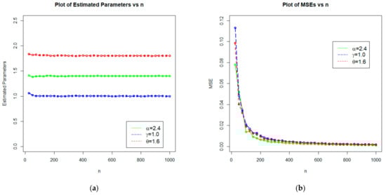
Figure 5. Plots of (a) estimated parameters vs. n, and (b) MSEs vs. n for Set 1: $\alpha =$ 1.4, $\gamma =$ 1.0, $\theta =$ 1.6.

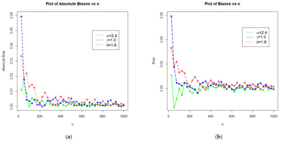
Figure 6. Plots of (a) absolute biases vs. n, and (b) biases vs. for Set 1: $\alpha =$ 1.4, $\gamma =$ 1.0, $\theta =$ 1.6.

Figure 7. Plots of (a) estimated parameters vs. n, and (b) MSEs vs. n for Set 2: $\alpha =$ 2.4, $\gamma =$ 1.7, $\theta =$ 1.5.

Figure 8. Plots of (a) absolute biases vs. n, and (b) biases vs. for Set 2: $\alpha =$ 2.4, $\gamma =$ 1.0, $\theta =$ 1.6.

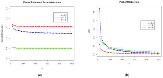
Figure 9. Plots of (a) estimated parameters vs. n, and (b) MSEs vs. n for Set 3: $\alpha =$ 0.5, $\gamma =$ 1.2, $\theta =$ 1.6.

Figure 10. Plots of (a) absolute biases vs. n, and (b) bias vs. n for Set 3: $\alpha =$ 0.5, $\gamma =$ 1.2, $\theta =$ 1.6.

From Table 1, we can see that as the sample size increase:

• The estimated values of $\hat{\alpha }MLE$, $\hat{\gamma }MLE$, and $\hat{\theta }MLE$ tend to be stable.

• The MSE of $\hat{\alpha }MLE$, $\hat{\gamma }MLE$, and $\hat{\theta }MLE$ decreases.

• The biases of $\hat{\alpha }MLE$, $\hat{\gamma }MLE$, and $\hat{\theta }MLE$ become smaller.

In conclusion, it is apparent that the MLEs perform reasonably well in estimating the model parameters of the NMEPA family of distributions.

5. Applications of NMEPA-Wei to Engineering Data

In order to demonstrate the usefulness of the NMEPA-Wei distribution for modeling, in this section, we analyzed two real data sets. The first data set is taken from Merovci et al. [26] and also used by Dey et al. [21], consisting of 63 observations of the strength of 1.5 cm glass fibers that were originally obtained by workers in the UK (National Physical Laboratory). While the second data set initially presented by Barlow et al. [27], was later on studied by Andrews and Herzberg [28], and then, later on, was also used by Dey et al. [21], represents the life of a fatigue fracture of Kevlar 373/epoxy that is subject to constant pressure at the 90 stress level until all had failed. For both data sets, see Table 2.

Table 2. The engineering data sets.

Data set 1

0.55, 0.74, 0.77, 0.81, 0.84, 0.93, 1.04, 1.11, 1.13, 1.24, 1.25, 1.27, 1.28, 1.29, 1.30, 1.36, 1.39, 1.42, 1.48, 1.48, 1.49, 1.49, 1.50, 1.50, 1.51, 1.52, 1.53, 1.54, 1.55, 1.55, 1.58, 1.59, 1.60, 1.61, 1.61, 1.61, 1.61, 1.62, 1.62, 1.63, 1.64, 1.66, 1.66, 1.66, 1.67, 1.68, 1.68, 1.69, 1.70, 1.70, 1.73, 1.76, 1.76, 1.77, 1.78, 1.81, 1.82, 1.84, 1.84, 1.89, 2.00, 2.01, 2.24

Data set 2

0.0251, 0.0886, 0.0891, 0.2501, 0.3113, 0.3451, 0.4763, 0.5650, 0.5671, 0.6566, 0.6748, 0.6751, 0.6753, 0.7696, 0.8375, 0.8391, 0.8425, 0.8645, 0.8851, 0.9113, 0.9120, 0.9836, 1.0483, 1.0596, 1.0773, 1.1733, 1.2570, 1.2766, 1.2985, 1.3211, 1.3503, 1.3551, 1.4595, 1.4880, 1.5728, 1.5733, 1.7083, 1.7263, 1.7460, 1.7630, 1.7746, 1.8275, 1.8375, 1.8503, 1.8808, 1.8878, 1.8881, 1.9316, 1.9558, 2.0048, 2.0408, 2.0903, 2.1093, 2.1330, 2.2100, 2.2460, 2.2878, 2.3203, 2.3470, 2.3513, 2.4951, 2.5260, 2.9911, 3.0256, 3.2678, 3.4045, 3.4846, 3.7433, 3.7455, 3.9143, 4.8073, 5.4005, 5.4435, 5.5295, 6.5541, 9.0960

The comparison of the proposed distribution is made with five well-known lifetime probability distributions, such as APT-Wei (Alpha Power Transformed Wei) proposed by Dey et al. [21], Ex-Wei (Exponentiated Wei) of Medholkar and Srivastava [3], classical Weibull (Wei) [14], Sarhan and Zaindin Modified Wei (Mod-Wei) [15], and Kumaraswamy Wei (Ku-Wei) distribution of Cordeiro et al. [16]. The CDFs of the competitor distributions are as follows:

• The APT-Wei distribution

  $$K\left(y;\alpha ,\gamma ,\theta \right)=\frac{{\alpha }^{\left(1-e^{-\gamma y^{\theta }}\right)}-1}{\alpha -1},\hspace{1em}\hspace{1em}y\ge 0,\alpha ,\theta ,\gamma >0.$$
• The Ex-Wei distribution

  $$K\left(y;\alpha ,\gamma ,\theta \right)={\left(1-e^{-\gamma y^{\theta }}\right)}^{\delta },\hspace{1em}\hspace{1em}y\ge 0,\delta ,\theta ,\gamma >0.$$
• The classical Wei distribution

  $$K\left(y;\gamma ,\theta \right)=\left(1-e^{-\gamma y^{\theta }}\right)\hspace{1em}\hspace{1em}y\ge 0,\gamma ,\theta >0.$$
• Sarhan and Zaindin Mod-Wei distribution

  $$K\left(y;\gamma ,\theta ,\delta \right)=\left(1-e^{-\gamma y^{\theta }-\delta y}\right)\hspace{1em}\hspace{1em}y\ge 0,\gamma ,\delta ,\theta >0.$$
• The Ku-Wei distribution

  $$K\left(y;a,b,\gamma ,\theta \right)=1-{\left(1-{\left(1-e^{-\gamma y^{\theta }}\right)}^a\right)}^b,y\ge 0,a,b,\gamma ,\theta >0.$$

Next, we consider different goodness of fit measures to examine which competitor is the best fit for the considered data sets. These goodness of fit measures include: CM (Cramer–von Misses) test statistic, AD (Anderson–Darling) test statistic, KS (Kolmogorov–Smirnov) test statistic, AIC (Akaike Information Criterion), BIC (Bayesian Information Criterion), corrected Akaike information criterion (CAIC), and HQIC (Hannan–Quinn information criterion) as well as p-values. The mathematical formulae of these measures are given by:

• The CM test statistic calculated as

$$CM={{\displaystyle \sum _{i=1}^n\left[\frac{2i-1}{2n}-G\left(y_i;\Delta \right)\right]}}^2+\frac{1}{12n}.$$

• The AD test statistics computed as

$$AD=-n-\frac{1}{n}{\displaystyle \sum _{i=1}^n\left(2i-1\right)}\times \left[\log G\left(y_i;\Delta \right)+\log \left(1-G\left(y_{i-n+1};\Delta \right)\right)\right].$$

• The KS test statistic derived as

$$\sup x[G_n\left(y;\Delta \right)-G\left(y;\Delta \right)].$$

• The AIC test statistics obtained as

$$AIC=2p-2L.$$

• The BIC test statistics derived as

$$BIC=p\log (n)-2L.$$

• The CAIC test statistics calculated as

$$CAIC=\frac{2np}{n-p-1}-2L.$$

• The HQIC test statistics computed as

$$HQIC=2p\log \left(\log (n)\right)-2L.$$

where L is the maximized likelihood function evaluated at MLEs, n is the sample size, and p is the number of parameters in the model. All of the above computations are carried out by the statistical R software using the (AdquacyModel) package with the “BFGS” algorithm. In general, a model having smaller values of these analytical measures and a higher p-value indicates the best fit among the other competitive models to the considered data sets.

5.1. Data 1

Corresponding glass fiber data set (Data 1), some basic measures of statistics for the first data set are the following: Minimum = 0.550, 1st Quartile = 1.375, Median = 1.590, Mean = 1.507, 3rd Quartile = 1.685, Maximum = 2.240, variance = 0.1050575, Range = 1.69, Skewness = −0.8999263, and Kurtosis = 3.923761. Corresponding to Data 1, some basic plots including histogram, Kernel density plot, TTT plot, Violin plot, and box plot for the first data set are presented in Figure 11. From Figure 11, it is clear that the data are negatively skewed and suffer from an increasing hazard rate. Thus, the proposed NMEPA-Wei model can be used to model HF of the first data set.

Figure 11. The (a) Histogram, (b) Kernel density plot, (c) TTT plot, (d) Violin plot, and (e) box plot for Data 1.

Furthermore, the values of $\hat{\gamma }MLE$, $\hat{\theta }MLE$, $\hat{\alpha }MLE$, $\hat{a}MLE$, $\hat{b}MLE$, and $\hat{\delta }MLE$ of the NMEPA-Wei and other competing models are reported in Table 3. While the numerical values of analytical and discrimination measures (taken to select the nice model) are presented in Table 4 and Table 5. The theoretical and empirical PDFs and CDFs plots of the NMEPA-Wei and other competitor models are displayed in Figure 12. The probability–probability plots of the proposed and competing models are displayed in Figure 13. Similarly, for the same data, the quantile–quantile (Q-Q) plots for the proposed and all the other competing models are presented in Figure 14.

Table 3. The values of $\hat{\gamma }MLE$, $\hat{\theta }MLE$, $\hat{\alpha }MLE$, $\hat{a}MLE$, $\hat{b}MLE$, and $\hat{\delta }MLE$ of the competitive models using glass fiber data set (Data 1).

Models	$\hat{\mathit{\gamma }}\mathit{M}\mathit{L}\mathit{E}$	$\hat{\mathit{\theta }}\mathit{M}\mathit{L}\mathit{E}$	$\hat{\mathit{\alpha }}\mathit{M}\mathit{L}\mathit{E}$	$\hat{\mathit{a}}\mathit{M}\mathit{L}\mathit{E}$	$\hat{\mathit{b}}\mathit{M}\mathit{L}\mathit{E}$	$\hat{\mathit{\delta }}\mathit{M}\mathit{L}\mathit{E}$
NMEPA-Wei	0.25201	4.47591	2.03312	-	-	-
APT-Wei	0.19403	4.48236	10.83013	-	-	-
Ex-Wei	0.02013	7.21201	-	-	-	0.68101
Wei	0.05980	5.77622	-	-	-	-
Mod-Wei	6.37653	0.03092	-	-	-	0.04083
Ku-Wei	0.11102	7.10514	-	0.50902	0.22313	-

Table 4. The goodness of fit CM, AD, and KS measures, and p-value of the competitive models for glass fiber data set (Data 1).

Models	CM	AD	KS	p-Values
NMEPA-Wei	0.0497	0.3355	0.1221	0.8685
APT-Wei	0.1682	0.9273	0.1472	0.2993
Ex-Wei	0.2013	1.1162	0.1524	0.1312
Wei	0.2373	1.3045	0.1332	0.1069
Mod-Wei	0.1385	0.7985	0.1332	0.2142
Ku-Wei	0.1493	0.8471	0.1221	0.2091

Table 5. The discrimination AIC, BIC, CAIC, and HQIC measures of competitive models using glass fiber data set (Data 1).

Models	AIC	BIC	CAIC	HQIC
NMEPA-Wei	27.1435	33.5729	27.5503	29.6722
APT-Wei	32.9483	39.3772	33.3553	35.4773
Ex-Wei	35.3521	41.7821	35.7592	37.8812
Wei	35.7893	38.7000	34.6137	36.0995
Mod-Wei	35.7892	42.2187	36.1961	38.3180
Ku-Wei	35.5131	44.0852	36.2023	38.8832

Figure 12. Plots of (a) estimated PDFs, and (b) estimated CDFs of competitive models for Data 1.

Figure 13. Probability–probability (PP) plots of (a) NMEPA-Wei, (b) APT-Wei, (c) Ex-Wei, (d) Wei, (e) Mod-Wei, and (f) Ku-Wei for Data 1.

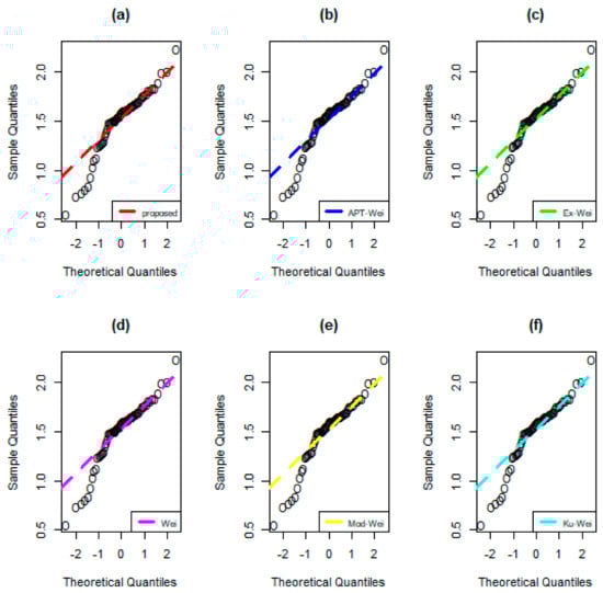
Figure 14. Q-Q (quantile–quantile) plots of (a) NMEPA-Wei, (b) APT-Wei, (c) Ex-Wei, (d) Wei, (e) Mod-Wei, and (f) Ku-Wei distributions for Data 1.

Based on the numerical results, obtained in Table 4 and Table 5, we can see that the NMEPA-Wei model has the lowest values of the analytical and discrimination measures. The values of the analytical measures for the NMEPA-Wei distribution are: AIC = 27.1435, BIC = 33.5729, CAIC = 27.5503, HQIC = 29.6722, CM = 0.0497, AD = 0.3355, KS = 0.1221, with p-value = 0.8685. In terms of AIC, BIC, CAIC, HQIC, and p-value, the second-best model is the APT-Wei distribution. The values of these measures for the APT-Wei distribution are given by 32.9483, 39.3772, 33.3553, 35.4773, and 0.2993. Whereas the second-best model in terms of CM, AD, and KS is the Mod-Wei distribution. For the Mod-Wei distribution, the CM, AD, and KS values are given by 0.1385, 0.7985, and 0.1332, respectively.

In support of numerical illustrations in Table 4 and Table 5 and the above discussion, we observed that the NMEPA-Wei distribution is the optimum choice for glass fiber data (Data 1). According to Figure 12, Figure 13 and Figure 14, it is observed that the NMEPA-Wei distribution fits the glass fiber data quite well.

5.2. Data 2

Corresponding fatigue fracture of Kelvar 373/epoxy data set (Data 2), some basic measures of statistics for the second data set are the following: minimum = 0.0251, 1st Quartile = 0.9048, median = 1.7362, mean = 1.9592, 3rd Quartile = 2.2959, maximum = 9.0960, variance = 2.477415, range = 9.0709, Skewness = 1.979558, and Kurtosis = 8.160792. Corresponding to Data 2, some basic plots including histogram, Kernel density plot, TTT plot, Violin plot, and box plot for the second fatigue fracture data set are presented in Figure 15. From Figure 15, it is clear that the data are positively skewed and suffer from an increasing hazard rate. Thus, the proposed NMEPA-Wei model can be used to model HF of the second data set.

Figure 15. The (a) Histogram, (b) Kernel density plot, (c) TTT plot, (d) Violin plot, and (e) box plot for Data 2.

Furthermore, the values of $\hat{\gamma }MLE$, $\hat{\theta }MLE$, $\hat{\alpha }MLE$, $\hat{a}MLE$, $\hat{b}MLE$, and $\hat{\delta }MLE$ of the NMEPA-Wei and other competing models are reported in Table 6. Whereas the numerical values of analytical and discrimination measures (taken to select the nice model) are presented in Table 7 and Table 8. The theoretical and empirical PDFs and CDFs plots of the NMEPA-Wei and other competitor models are displayed in Figure 16. The P-P (probability–probability) plots of the proposed and competing models are displayed in Figure 17. Similarly, for the same data, the Q-Q (quantile–quantile) plots for the proposed and all the other competing models are sketched in Figure 18.

Table 6. The values of $\hat{\gamma }MLE$, $\hat{\theta }MLE$, $\hat{\alpha }MLE$, $\hat{a}MLE$, $\hat{b}MLE$, and $\hat{\delta }MLE$ of the competitive models using fatigue fracture data set (Data 2).

Models	$\hat{\mathit{\gamma }}\mathit{M}\mathit{L}\mathit{E}$	$\hat{\mathit{\theta }}\mathit{M}\mathit{L}\mathit{E}$	$\hat{\mathit{\alpha }}\mathit{M}\mathit{L}\mathit{E}$	$\hat{\mathit{a}}\mathit{M}\mathit{L}\mathit{E}$	$\hat{\mathit{b}}\mathit{M}\mathit{L}\mathit{E}$	$\hat{\mathit{\delta }}\mathit{M}\mathit{L}\mathit{E}$
NMEPA-Wei	1.85724	0.66292	2.59681	-	-	-
APT-Wei	0.09442	1.59063	0.02183	-	-	-
Ex-Wei	0.57967	1.10123	-	-	-	1.4426 4
Wei	0.36633	1.32560	-	-	-	-
Mod-Wei	0.43131	1.28260	-	-	-	−0.06313
Ku-Wei	1.78175	3.75453	-	0.30474	0.88932	-

Table 7. The values of CM, AD, and KS measures and p-value of the competitive models for fatigue fracture data set (Data 2).

Models	CM	AD	KS	p-Values
NMEPA-Wei	0.0563	0.3335	0.0798	0.6872
APT-Wei	0.0901	0.5378	0.0821	0.6533
Ex-Wei	0.1167	0.6912	0.0987	0.4217
Wei	0.1305	0.7672	0.1099	0.2953
Mod-Wei	0.1304	0.7676	0.1083	0.3112
Ku-Wei	0.1137	0.6737	0.0972	0.4403

Table 8. The discrimination measures values of AIC, BIC, CAIC, and HQIC measures of competitive models using fatigue fracture data set (Data set 2).

Models	AIC	BIC	CAIC	HQIC
NMEPA-Wei	247.9672	254.9594	248.3005	250.7616
APT-Wei	248.7293	255.7212	249.0623	251.5234
Ex-Wei	250.3272	257.3194	250.6606	253.1216
Wei	249.0494	253.7108	249.2138	250.9123
Mod-Wei	251.0238	258.0160	251.3571	253.8182
Ku-Wei	252.1412	261.4642	252.7046	255.8671

Figure 16. Plots of (a) estimated PDFs, and (b) estimated CDFs of competitive models for Data 2.

Figure 17. Probability–probability (PP) plots of (a) NMEPA-Wei, (b) APT-Wei, (c) Ex-Wei, (d) Wei, (e) Mod-Wei, and (f) Ku-Wei for Data 2.

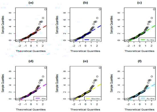
Figure 18. Q-Q (quantile–quantile) plots of (a) NMEPA-Wei, (b) APT-Wei, (c) Ex-Wei, (d) Wei, (e) Mod-Wei, and (f) Ku-Wei distributions for Data 2.

Again, if we look at the numerical results obtained in Table 7 and Table 8, it is obvious that the NMEPA-Wei model has the lowest values of the analytical measures and the highest p-value. The values of the analytical measures for the NMEPA-Wei distribution are: AIC = 247.9672, BIC = 254.9594, CAIC = 248.3005, HQIC = 250.7616, CM = 0.0563, AD = 0.3335, KS = 0.0798, with p-value = 0.6872. In terms of AIC, CAIC, CM, AD, KS, and p-value, the second-best model is also the APT-Wei distribution. The values of these measures for the APT-Wei distribution are given by 248.7293, 249.0623, 0.0901, 0.5378, 0.0821, and p-value = 0.6533. Whereas the second-best model in terms of BIC and HQIC is the classical Wei distribution. For the Wei distribution, the BIC, and HQIC values are given by 253.7108, and 250.9123, respectively.

From the numerical illustrations given in Table 7 and Table 8 and the above discussion, we can conclude that the NMEPA-Wei distribution is a good choice for analyzing or examining the fatigue fracture of Kelvar 373/epoxy data (Data 2). According to Figure 16, Figure 17 and Figure 18, it is also observed that the NMEPA-Wei distribution fits the fatigue fracture of Kelvar 373/epoxy data quite well.

6. Conclusions

In the present work, we have presented a new family of distributions called the New Modified Exponent Power Alpha family (NMEPA). A three-parameter special sub-case of the proposed class by employing the Weibull distribution as a baseline distribution is studied in detail. The special sub-case is named as NMEPA-Wei (new modified exponent power Alpha Wei) distribution. The PDF (probability density function) of the derived model is positively skewed, negatively skewed, symmetrical, and also bimodal depending upon parameter values. Moreover, the HF (hazard function) can have non-monotonically increasing, decreasing, uni-model, and bathtub shapes. General expressions, for different statistical properties of the proposed family, have been derived including quantile function, moments, moments generating function, and order statistics. The Maximum Likelihood method has been used for estimating the unknown parameters, and in addition, a Monte Carlo simulation study is carried out to assess the performance of the proposed model estimators. Based on analytical measures and graphical illustration, it is observed that the proposed NMEPA-Wei distribution is the best competitor for modeling the reliability of engineering data sets. We hope that this novel improvement in the field of distributions theory will provide more attractive applications in the reliability of engineering and other related fields.

References

- Lee, C.; Famoye, F.; Olumolade, O. Beta-Weibull distribution: Some properties and applications to censored data. J. Mod. Appl. Stat. Methods 2007, 6, 17. [Google Scholar] [CrossRef]
- Hussein, M.; Elsayed, H.; Cordeiro, G.M. A new family of continuous distributions: Properties and estimation. Symmetry 2022, 14, 276. [Google Scholar] [CrossRef]
- Shah, Z.; Ali, A.; Hamraz, M.; Khan, D.M.; Khan, Z.; EL-Morshedy, M.; Al-Bossly, A.; Almaspoor, Z. A New Member of TX Family with Applications in Different Sectors. J. Math. 2022, 2022, 1453451. [Google Scholar] [CrossRef]
- Ahmad, Z.; Mahmoudi, E.; Kharazmi, O. On modeling the earthquake insurance data via a new member of the TX family. Comput. Intell. Neurosci. 2020, 2020, 7631495. [Google Scholar] [CrossRef] [PubMed]
- Wang, W.; Ahmad, Z.; Kharazmi, O.; Ampadu, C.B.; Hafez, E.H.; Mohie El-Din, M.M. New generalized-x family: Modeling the reliability engineering applications. PLoS ONE 2021, 16, e0248312. [Google Scholar] [CrossRef]
- Eghwerido, J.T.; Efe-Eyefia, E.; Zelibe, S.C. The transmuted alpha power-G family of distributions. J. Stat. Manag. Syst. 2021, 24, 965–1002. [Google Scholar] [CrossRef]
- Guerra, R.R.; Peña-Ramírez, F.A.; Bourguignon, M. The unit extended Weibull families of distributions and its applications. J. Appl. Stat. 2021, 48, 3174–3192. [Google Scholar] [CrossRef]
- Mohammed, H.S.; Ahmad, Z.; Abdulrahman, A.T.; Khosa, S.K.; Hafez, E.H.; Abd El-Raouf, M.M.; El-Din, M.M.M. Statistical modelling for Bladder cancer disease using the NLT-W distribution. AIMS Math. 2021, 6, 9262–9276. [Google Scholar] [CrossRef]
- Mudholkar, G.S.; Srivastava, D.K. Exponentiated Weibull family for analyzing bathtub failure-rate data. IEEE Trans. Reliab. 1993, 42, 299–302. [Google Scholar] [CrossRef]
- Cordeiro, G.M.; de Castro, M. A new family of generalized distributions. J. Stat. Comput. Simul. 2011, 81, 883–898. [Google Scholar] [CrossRef]
- Nofal, Z.M.; Afify, A.Z.; Yousof, H.M.; Granzotto, D.C.; Louzada, F. Kumaraswamy transmuted exponentiated additive Weibull distribution. Int. J. Stat. Probab. 2016, 5, 78–99. [Google Scholar] [CrossRef]
- Cordeiro, G.M.; Ortega, E.M.; Nadarajah, S. The Kumaraswamy Weibull distribution with application to failure data. J. Frankl. Inst. 2010, 347, 1399–1429. [Google Scholar] [CrossRef]
- El-Damcese, M.A.; Mustafa, A.; El-Desouky, B.S.; Mustafa, M.E. The Kumaraswamy flexible Weibull extension. Int. J. Math. Appl. 2016, 4, 1–14. [Google Scholar]
- Selim, M.A.; Badr, A.M. The Kumaraswamy generalized power Weibull distribution. Math. Theo. Model 2016, 6, 110–124. [Google Scholar]
- Marshall, A.W.; Olkin, I. A new method for adding a parameter to a family of distributions with application to the exponential and Weibull families. Biometrika 1997, 84, 641–652. [Google Scholar] [CrossRef]
- Ghitany, M.E.; Al-Hussaini, E.K.; Al-Jarallah, R.A. Marshall–Olkin extended Weibull distribution and its application to censored data. J. Appl. Stat. 2005, 32, 1025–1034. [Google Scholar] [CrossRef]
- Gui, W. Marshall-Olkin extended log-logistic distribution and its application in minification processes. Appl. Math. Sci. 2013, 7, 3947–3961. [Google Scholar] [CrossRef]
- Saboor, A.; Pogány, T.K. Marshall–Olkin gamma–Weibull distribution with applications. Commun. Stat. Theory Methods 2016, 45, 1550–1563. [Google Scholar] [CrossRef]
- Khan, S.; Balogun, O.S.; Tahir, M.H.; Almutiry, W.; Alahmadi, A.A. An alternate generalized odd generalized exponential family with applications to premium data. Symmetry 2021, 13, 2064. [Google Scholar] [CrossRef]
- Alzaatreh, A.; Lee, C.; Famoye, F. A new method for generating families of continuous distributions. Metron 2013, 71, 63–79. [Google Scholar] [CrossRef]
- Dey, S.; Sharma, V.K.; Mesfioui, M. A new extension of Weibull distribution with application to lifetime data. Ann. Data Sci. 2017, 4, 31–61. [Google Scholar] [CrossRef]
- Weibull, W.A. Statistical distribution function of wide applicability. J. Appl. Mech. 1951, 18, 293296. [Google Scholar] [CrossRef]
- Sarhan, A.M.; Zaindin, M. Modified Weibull distribution. Appl. Sci. 2009, 11, 2336. [Google Scholar]
- Dong, B.; Ma, X.; Chen, F.; Chen, S. Investigating the differences of single-vehicle and multivehicle accident probability using mixed logit model. J. Adv. Transp. 2018, 2018, 2702360. [Google Scholar] [CrossRef]
- Doornik, J.A. An Object-Oriented Matrix Programming Language Ox 6; University of Oxford: Oxford, UK, 2009. [Google Scholar]
- Merovci, F.; Khaleel, M.A.; Ibrahim, N.A.; Shitan, M. The beta Burr type x distribution properties with applications. Springer Plus 2016, 5, 697. [Google Scholar] [CrossRef]
- Paul, D.R.; Barlow, J.W. A binary interaction model for miscibility of copolymers in blends. Polymer 1984, 25, 487–494. [Google Scholar] [CrossRef]
- Andrews, D.F.; Herzberg, A.M. Data: A Collection of Problems from Many Fields for the Student and Research Worker; Springer: Berlin/Heidelberg, Germany, 2012. [Google Scholar]
Publisher’s Note: MDPI stays neutral with regard to jurisdictional claims in published maps and institutional affiliations. |
© 2022 by the authors. Licensee MDPI, Basel, Switzerland. This article is an open access article distributed under the terms and conditions of the Creative Commons Attribution (CC BY) license (https://creativecommons.org/licenses/by/4.0/).