Abstract
For the purpose of studying the dynamic and inner flow features of an open inlet channel axial flow pump unit, in the present study, numerical calculations using the SST k-ω turbulence model are applied to an open inlet channel axial flow pumping unit based on the NS equation, and experimental validation is then performed. The experimental output indicates that the designed working conditions are Q = 350 L/s, head H = 5.065 m, efficiency η = 79.56%, and the maximum operating head is H = 9.027 m, which is about 1.78 times that of the design head; further, the pump device can operate in a wide range of working conditions. In addition, the design working conditions are within the range of high-efficiency operating conditions. The calculated values and the experimental comparison are all within a 5.0% margin of error; further, the numerical calculations are reliable. The hydraulic loss of the inlet channel under the design condition Q = 350 L/s is 0.0676 m, which satisfies the relationship of the quadratic function. The uniformity of the impeller inlet velocity is 80.675%, and the weighted average angle of the velocity is 79.223°. The hydraulic loss of the outlet channel under the design condition Q = 350 L/s is 0.3183 m, and the hydraulic loss curve is a parabola with an upward opening. The flow state of the pump device is sensitive to changes in the working conditions; additionally, the flow state is optimal under the design working conditions. In this study, the energy and inner flow features of the open inlet axial flow pumping units are revealed, and the research outcomes can be used as a reference for the design and operation of similar pumping units.
1. Introduction
The inlet channel is one of the more important components of a pump station. A reasonably designed inlet channel can provide a good inlet condition for the pump device and make the water flow into the pump as smoothly as possible. In addition, not only will this reduce the hydraulic loss, but it will also have a great impact on the overall flow state of the device. If the design of the inlet channel is not reasonable, however, then it will lead to water turbulence, a poor flow pattern, and will even—in serious cases—be accompanied by the generation of a vortex, which seriously affects the performance of the pump device. As the open water inlet structure is simple, has a convenient construction, and possesses technical requirements that are easy to meet, the open water inlet is currently, as a result, a widely used type of water inlet channel.
Certain scholars have conducted relevant studies on, for example, the optimal dimensions of open inlet channels. These dimensions have been summarized through experimental studies [1]. The design criteria for inlet channels have also been summarized [2,3], and reasonable suggestions have also been given for the other indicators of inlet channels. Other scholars have also numerically optimized various parameters of the inlet channel and have explored the effects of the back wall distance and back wall shape [4,5], bottom slope [6], and horn pipe height [7] values in regard to the hydraulic performance. Certain other scholars have studied axial flow pumps and investigated the effect of inlet channel conditions [8] via numerical calculations in order to investigate the behavior of axial flow pumps. These same scholars have concluded, through experiments, that changing the size of a vertical axial flow pump [9] causes changes in the flow velocity and fluid pressure in the pipe. Some scholars have numerically solved the internal flow field of vertical axial flow pump devices. They have also explored the influence of speed [10], under low-flow conditions, on the devices’ internal flow field; obtained the change rule of the pump’s performance [11] under different deflection angles; and studied the pressure allocation and distortion characteristics of different surfaces of the blade via fluid–solid coupling [12], thereby deriving the pressure zone distribution law. Relevant scholars have also studied the free surface vortex [13,14] as well as the internal vortex structure [15] of the pump sump through numerical calculations [16]; further, they have also photographed the evolution process of the underwater suction vortex [17] of the axial flow pump device, providing a theoretical basis for the prevention of the suction vortex being generated.
The optimal design of open inlet channels has been studied by many scholars, but the internal flow characteristics are less well understood. Based on the NS equation [18], this study adopts an SST k-ω [19] turbulence model, which is used to conduct numerical calculations for an open inlet channel axial flow pump device and to analyze the internal flow characteristics of an open inlet channel. The hydraulic performance and internal flow characteristics of an open inlet channel axial flow pump device under different flow rates are obtained, which can provide theoretical guidance for the design and operation of the similar pump stations.
2. Numerical Computing Module, Meshing, and Calculation Approach
2.1. Numerical Computational Modules
The axial flow pump rig contains an open inlet channel, impeller, guide leaf, and outlet elbow parts. The nominal diameter of the impeller is recorded as D = 300 mm, the number of impeller blades is 4, and the number of guide leaf blades is 7. The detailed design parameters of these components are displayed in Table 1.

Table 1.
Detailed information regarding the pump unit.
In this study, the models of the inlet water channel, inlet flare pipe, and outlet bend are established by Solidworks. The models of the impeller and guide leaf are established by ANSYS TurboGrid [20], and the overall calculated 3D model is indicated in Figure 1, the pump rig position parameters are shown in Table 2.
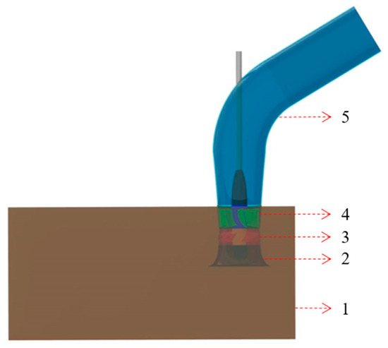
Figure 1.
Three-dimensional diagram of the calculation model. (1) Open water inlet channel; (2) inlet flare; (3) impeller; (4) guide leaf; and (5) outlet bend.
Table 2.
Pump rig position parameters.
2.2. Mesh Division
The open inlet channel and flare pipe are divided by unstructured grids in ICEM [21]. Further, the outlet bend is divided by structured grids in ICEM, and the impeller and guide leaf are divided by structured grids in Turbogrid. Grid diagram of calculation model is shown in Figure 2.
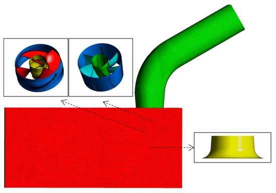
Figure 2.
Grid diagram of calculation model.
The numerical calculation domain consists of 5 parts, which are the: open inlet channel, inlet flare pipe, impeller domain, guide leaf domain, and outlet bend. In order to meet the requirements of calculation accuracy, the “J” topology is adopted near the impeller blade, the “O” topology is adopted for the guide leaf blade, and the “H” topology is adopted at the impeller tip clearance, where eight layers of grids are arranged. The key parts of the blade are densified to ensure that the average y+ of the grid at the impeller tip clearance does not exceed 10. The average y+ value of the impeller and guide leaf surface is about 50 (y+ is a measureless number of distance to the wall, which is direct to the first mesh height of the surface of the wall; in the numerical computation with the SST k-ω and RNG k-ε turbulent current mode, the rotational and shear flow y+ is taken as 30~100). After the grid independence [22] analysis was conducted, the efficiency of the pump unit changed slightly after the grid number became 3,009,738 (i.e., the grid number of the impeller was 1,604,312, the grid number of the guide leaf was 442,491, the grid number of the outlet bend was 212,750, the grid number of the bell mouth was 360,384, and the grid number of the inlet channel was 389,801). Therefore, a grid number of 3,009,738 was selected for the subsequent numerical calculations in this study. The grid independence analysis graph is shown in Figure 3 (flow condition Q = 300 L/s).
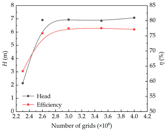
Figure 3.
Grid irrelevance analysis.
2.3. Control Equations and Boundary Conditions
In the calculation, the grid mode of the components is introduced into CFX-Pre, which combines the meshes of each section to form the numerical calculation model of the pump unit. Moreover, the numerical calculation settings and boundary conditions are detailed in Table 3.
Table 3.
Numerical computation setup and boundary conditions.
In this study, four different models were used for the purposes of the grid irrelevance analysis. Further, the results were fitted to the experimental efficiency value, where k-ε and k-ω were 76.673% and 76.418%, respectively. The efficiencies of SST k-ω and RNG k-ε were closer to the test efficiencies of 77.62%, 77.463%, and 77.468%, respectively. Considering the high accuracy required for solving the flow near the wall, the SST k-ω [23] model of turbulent flow was used for the numerical computation of the open inlet channel axial flow pump unit. The spreading items and the press force ramps are indicated using the finite element-based finite volume approach; additionally, the high-resolution format (i.e., a high resolution scheme) is used for the flow items. In the computation, the stress of the stream of the field is P; the speeds of the x, y, and z orientations are u, v, and w, respectively; and the condition of confluence for the equation of the kinetic energy of the turbulence and the consumption rate ε is set to 10−5. In regard to the former, as a matter of principle, the less the remaining difference is, the more desirable it is.
2.4. Calculation Method
The pump equipment head Hnet [24] is calculated as:
The pump equipment efficiency η [25] is calculated as:
where P1 and P2 mean the hydrostatic pressure at the intake and outtake of the axial pump flow tunnel (in Pa); ρ is the water density (in kg/m3); g is the acceleration of gravity (in m/s2); s1 and s2 are the axial flow pump intake and outtake cross-sectional area (in m2); u1 and u2 are the flow velocity at each point of the inlet and outlet section of the axial pump (in m/s); ut1 and ut2 are the normal components of the flow velocity at each point of the inlet and outlet section of the axial pump (in m/s); Q is the flow rate of the axial pump (in m3/s); T is the impeller rotational torque (in N·m); and ω is the rotation angular velocity of the impeller (in rad/s).
The uniformity of the axial flow velocity distribution [26] is calculated as:
where Vzu is the uniformity of the axial flow velocity distribution at the exit section of the runner; is the arithmetic mean of axial flow velocity at the exit section of the runner; vai is the axial velocity (in m/s) of each calculation unit at the exit section of the runner; and n is the number of calculation units at the exit section of the runner.
The velocity-weighted average angle [27,28] is calculated as:
where uti is the transverse velocity (in m/s) of each unit in the characteristic section of the flow channel and uai is the axial velocity of unit i (in m/s).
The hydraulic loss hf [29,30] is calculated as:
where E1 and E2 are the total energy at the inlet and outlet of the open flow channel; Z1 and Z2 are the height of the inlet and outlet of the open flow channel (in m); and u1 and u2 are the inlet and outlet water velocity of the open flow channel (in m/s).
3. Test Rig and Test Approach
3.1. Test Rig
The test rig is a standing closed loop system, as illustrated in Figure 4.
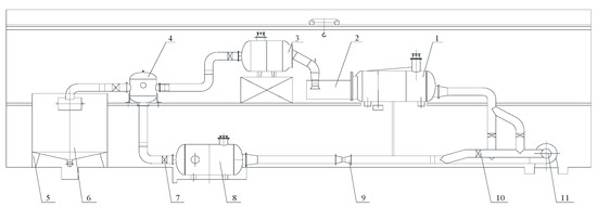
Figure 4.
High accuracy hydraulic machinery test bench plan. (1) Inlet unit; (2) test pump equipment; (3) the pressure discharge box; (4) forking water tank; (5)~(6) flow calibration unit in situ; (7) service regulation gate valve; (8) steady voltage rectifier barrel; (9) the electromagnetic meters of flow; (10) running control gate valve; and (11) accessory pump unit.
The differential pressure transmitter (accuracy ± 0.015%) is used to measure the head in the test; the flow rate is measured using the electro-magnetic flowmeter (accuracy ± 0.18%) measurement; the velocity and torque are calculated using speed and torque sensors (accuracy ± 0.24%); and the integrated uncertainty of the test bench is measured at ± 0.39%.
3.2. Experimental Test Approach
The head of the pump unit H [31,32] can be computed by the following equation:
The pump unit axial power N [33] can be computed by the following formula:
The efficiency η [34,35] is calculated as:
where M is the input torsion of the pump (in N·m); M’ is the pump mechanical losing torsional moment (in N·m); n is the pump experimental revolution speed (in r/min); η is the pump model efficiency (in %); Q is the pump flow rate (in m3/s); H is the head of the pump (in m); ρ is the test of the densities of the body of water in real time (in kg/m3); and g is the acceleration of gravity at the location (in m/s2).
4. Pump Unit Energy and Internal Flow Characteristic Analysis
4.1. Pump Unit Energy Characteristic Analysis
Following the numerical computation results, Equations (1) and (2) were used to compute the numerical computation head and efficiency of the axial flow pump units, as shown in Table 4. The test parameters under different flow conditions were obtained through the test, and the test head and efficiency of the axial flow pump unit were calculated using Equations (6)–(8), as illustrated in Table 4. A comparison of the numerical calculations and the test energy characteristics is displayed in Figure 5.
Table 4.
Numerical calculations and experimental energy characteristics.
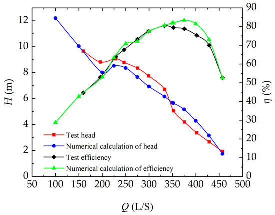
Figure 5.
Comparison of experimental and numerical calculations.
According to the test results shown in Table 4, the highest efficiency working condition of the pump unit is Q1 = 333.27 L/s, head H1 = 6.718 m, and efficiency η1 = 80.38%. After the origin interpolation analysis is conducted, we can obtain the design working condition Q2 = 350 L/s, head H2 = 5.065 m, and efficiency η2 = 79.56% as outlined in Table 1. Further, we can obtain the axial flow pump design working condition Q3 = 350 L/s, head H3 = 5.0 m, and efficiency η3 = 80.0% at the time the difference in the head is ΔH = 0.065 m and the efficiency difference is Δη = 0.44%. This indicates that the design point is accurate. Moreover, the difference between the efficiency of the highest efficiency working point and the efficiency of the design working point Δη = 0.82% indicates that the design working condition is within the high-efficiency operating condition, thereby meeting the design requirements. The maximum working head is at the beginning of the saddle area—corresponding to a head of H4 = 9.027 m—which is about 1.78 times that of the design head; this, therefore, indicates that the pump unit can operate in a wider range of conditions, which is more conducive to the efficient, stable, and safe operation of the pump unit.
The comparative analysis displayed in Table 4 and Figure 5 shows that the test head is slightly higher than is shown in the numerical calculations in respect to the low-flow condition (Q = 100~330 L/s). Although the test efficiency is slightly lower than the numerical calculation in the high-flow condition (Q = 330~457 L/s), the difference between the efficiency in the flow condition (Q = 100~330 L/s and Q = 400~457 L/s) is not significant. In addition, the difference in the flow condition (Q = 330~400 L/s) shows the difference increases; further, the numerical calculation efficiency is higher than the test value and the error margins of both the numerical calculation and test comparison are within 5.0%. As such, in summary, the error values of the numerical calculation and test measurement established in this study is small and, therefore, the numerical calculation results are credible.
According to the numerical calculation results, the axial flow velocity distribution uniformity, velocity weighted average angle, and inlet channel hydraulic loss at the impeller inlet of the axial flow pump unit are calculated using Equations (3)–(5), respectively. These results are displayed in Table 5, according to which Figure 6 and Figure 7 can be drawn.
Table 5.
Uniformity of flow velocity distribution and velocity average weighted angle.
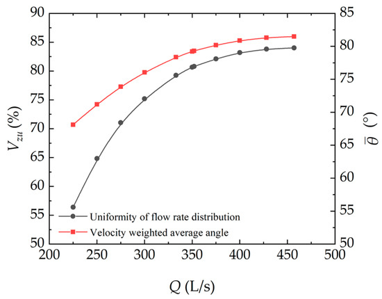
Figure 6.
Uniformity of flow velocity distribution and velocity weighted average angle under different working conditions.
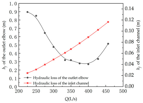
Figure 7.
Hydraulic losses in the inlet channel under different working conditions.
The design of the inlet channel should take into account the small hydraulic loss, while also providing uniform flow inlet conditions for the impeller. The outlet of the inlet channel is the inlet of the impeller chamber, and its axial velocity distribution uniformity, Vzu, reflects the advantages and disadvantages of the inlet channel design. The closer Vzu is to 100%, the more uniform the axial velocity distribution of the inlet channel outlet water flow, and the more uniform the water flow into the impeller in the same direction. As shown in Table 5 and Figure 6, we can see that the uniformity of the flow velocity at the impeller inlet of the open inlet channel increases gradually with the flow rate. It was recorded as 80.675% for the design working condition (Q = 350 L/s) and the streamline can enter the impeller domain evenly. The open inlet channel axial flow pump rig, when compared to the axial flow pump, increased the open inlet channel and inlet flare, resulting in the axial flow pump impeller inlet conditions becoming worse. Additionally, as displayed in Table 5, it can be seen that in the axial flow pump rig impeller inlet the flow velocity uniformity is only 80.675%, which is the ideal state for when the axial flow pump impeller inlet flow velocity uniformity is close to 100%. When compared to the axial flow pump, the pump rig not only increased the open inlet channel hydraulic losses, but also the part, impeller, guide leaf, and outlet channel due to the increase in the bad flow state. Further, hydraulic losses will also increase and ultimately lead to a lower head and lower efficiency.
In addition, the axial velocity weighted average angle, θ, reflects the design quality of the inlet channel Moreover, the closer it is to 90°, the better the directional velocity of the outlet flow of the inlet channel is. From Table 5 and Figure 6, it can be seen that the velocity-weighted average angle at the impeller inlet is as low in the low-flow condition (Q = 100~330 L/s); however, this gradually improves with the increase in the flow rate. In regard to the design condition (Q = 350 L/s), the velocity-weighted average angle reaches 79.223°, and the curve increment decreases, also the value of velocity-weighted average angle at the high-flow condition (Q = 350~457 L/s) remains essentially flat. The velocity-weighted average angle at the outlet of the inlet channel, under the design working condition (Q = 350 L/s), could indicate that the inlet channel can provide good water inlet conditions for the impeller.
The Inlet and outlet channel hydraulic losses is shown in Table 6, through Table 6 and Figure 7, we can see that the hydraulic loss of the inlet channel satisfies the quadratic function and that the hydraulic loss curve of the inlet channel can be obtained by fitting hf = 0.5517 Q2 (fit: R = 0.9958, Q unit: m3/s, and hf unit: m). Further, the hydraulic loss of the inlet channel is 0.0676 m when at the design condition (Q = 350 L/s). In addition, when the hydraulic loss of the outlet bend meets the opening upward parabola, through which the fitting can be derived from the outlet bend, the hydraulic loss curve is hf = 29.439Q2 − 22.27Q + 4.4992 (fit: R = 0.9599, Q unit: m3/s, and hf unit: m). Moreover, the outlet bend hydraulic loss is 0.3183 m and the design conditions (Q = 350 L/s) near the outlet channel hydraulic loss curve are located at the bottom of the parabola, indicating the smallest instance of hydraulic loss.
Table 6.
Inlet and outlet channel hydraulic losses.
4.2. Analysis of the Internal Flow Characteristics of the Pump Unit
In the numerical calculation results of the open inlet channel axial flow pump unit, the flow rates of Q = 250 L/s (0.714 Qd), Q = 300 L/s (0.857 Qd), Q = 350 L/s (1.0 Qd), Q = 400 L/s (1.143 Qd), and Q = 450 L/s (1.223 Qd) show that five conditions were selected for the analysis of the internal flow characteristics of the pump unit. In order to better analyze the internal flow characteristics of the open inlet channel, three typical sections were selected, as illustrated in Figure 8. Here, A1 is the horizontal section over the center of the impeller, A2 is the longitudinal section perpendicular to the incoming flow direction over the center of the impeller, and A3 is the longitudinal section parallel to the incoming flow direction over the impeller center.
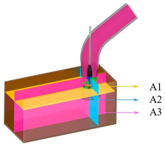
Figure 8.
Schematic diagram of the A1–A3 sections.
The streamlines and velocity distribution of the open inlet channel axial flow pump unit at flow conditions Q = 250 L/s (0.714 Qd), Q = 300 L/s (0.857 Qd), Q = 350 L/s (1.0 Qd), Q = 400 L/s (1.143 Qd), and Q = 450 L/s (1.223 Qd) for sections A1–A3 are illustrated in Figure 9, Figure 10 and Figure 11.
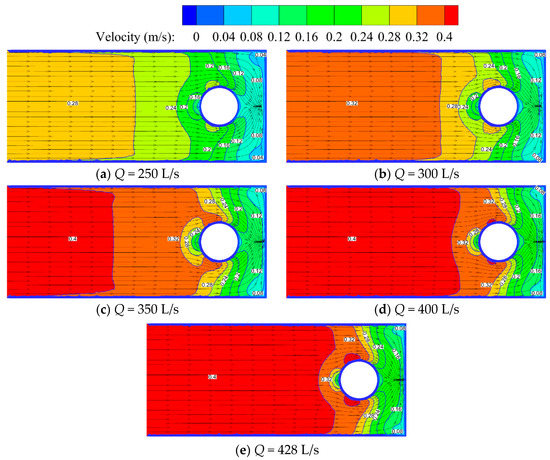
Figure 9.
Velocity flow diagram of A1 section with different flow conditions.
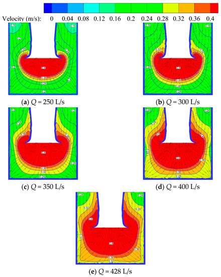
Figure 10.
Flow diagram of A2 section at different flow conditions.
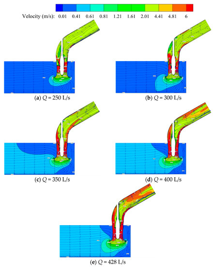
Figure 11.
A3 sectional velocity and streamline distribution.
As demonstrated in Figure 9, it can be seen that the open inlet channel has a more uniform distribution for each flow streamline on the left side of the impeller domain. Moreover, there is a vortex at the center of the rear wall due to the backflow of water hitting the rear wall between the right side of the impeller domain and the rear wall. The side wall of the flow channel, near the wall surface due to the side wall effect, the wall velocity is close to zero, whereas the side wall flow velocity stratification is greater, therefore illustrating uniform gradient changes. The streamline and velocity distribution of the open inlet channel illustrate the axisymmetric distribution along the central axis of the inlet channel, which indicates that the numerical calculation results are in accordance with the fluid mechanics theory.
As shown in Figure 9, in the low-flow working condition (Q = 250~350 L/s), the stratification effect of flow velocity in the inlet channel near the impeller domain is more obvious. However, the flow velocity distribution is not uniform as there is a semi-circular low-velocity area in front of the impeller domain and there are two symmetrical semi-circular high-velocity areas on the left and right sides of the impeller domain. In addition, both sides of the back wall of the flow channel is a slow velocity zone, the back wall zone has less water movement, and is approximately a stagnant water zone. Under the design condition (Q = 350 L/s), the stratification effect of flow velocity in the inlet channel near the impeller domain is improved, and there is only a low-velocity semicircular region in front of the impeller domain. There is no sudden change in flow velocity in the region on the left and on the right sides of the impeller domain. Further, the flow velocity in the back wall region increases, but it is still small. In the high-flow working condition (Q = 350~428 L/s), the stratification effect of flow velocity in the inlet channel near the impeller domain is further improved. In addition, the area of the low-velocity semi-circular region in front of the impeller domain is reduced, but there are two symmetrical high-velocity semi-circular regions on the left and right sides of the impeller domain, and the low-velocity region in the back wall area is further reduced. There is a vortex area at the center of the back wall under each working condition; however, the location and size of the vortex area remain essentially similar as the flow rate increases.
As seen in Figure 10, it can be determined that the flow velocity is higher near the inlet flare, under each working condition, and the high-velocity area is distributed in a ring shape, which decreases in a gradient from the center of the flare to the surroundings. With the increase in the flow, the ring area of the high-speed area gradually increases. From the distribution of streamlines in Figure 10, it can also be demonstrated that the streamlines contract towards the flare mouth and that the top streamline of the inlet channel is more uniform compared to the bottom.
As per Figure 11, it can be seen that the internal flow speed of the open inlet channel is lower, the streamline before the flare inside the inlet channel is more uniformly distributed, the streamline inside the inlet channel is gathered from all around to the flare, and the flow velocity near the flare is obviously increased in a gradient. Further, the water obtains kinetic energy at the impeller; the flow velocity reaches the maximum; and the guide lobe recovers the ring volume and converts part of the kinetic energy into pressure energy. Moreover, the flow velocity at the guide lobe is reduced compared with that at the impeller and, until the water flow into the outlet bend, the flow rate is further reduced. One of the reasons for this is because the internal flow line of the outlet channel is more complex. In addition, the flow pattern is poor and the fluid masses hit one another. However, on the other hand, the kinetic energy is reduced because the kinetic energy is further transformed into pressure energy and position potential energy, which also means that the velocity is reduced.
At low flow rates (Q = 250~350 L/s), there is significant outflow and backflow at the outlet of the guide leaf due to the low flow rate. In regard to the design conditions (i.e, Q = 350 L/s) and at high flow rates (Q = 350~428 L/s) the outflow phenomenon is improved and almost disappears; further, the streamlines inside the impeller and guide leaf are more uniform. In the small flow condition (Q = 250~350 L/s) and the design working condition (Q = 350 L/s), flow velocity distribution at the outlet of the bend outlet channel is more uniform compared with the high-velocity condition (Q = 350~428 L/s), and there is no vortex in the bend outlet channel, which means that the flow pattern of the outlet is comparatively reasonable. In addition, there is an obvious high-velocity and low-velocity interaction zone inside the bend outlet channel in the high-flow condition (Q = 350~428 L/s). Moreover, the flow velocity distribution is not uniform, which seriously affects the conversion of kinetic energy and the recovery of pressure energy of the outlet. In summary, the flow pattern of the discharge water under the design condition (Q = 350 L/s) is relatively good, which can also be illustrated by the hydraulic loss curve of the outlet channel, as shown in Figure 7.
The 3D streamlines of the open inlet axial flow pump unit at flow conditions Q = 250 L/s (0.714 Qd), Q = 300 L/s (0.857 Qd), Q = 350 L/s (1.0 Qd), Q = 400 L/s (1.143 Qd), and Q = 450 L/s (1.223 Qd) are illustrated in Figure 12.
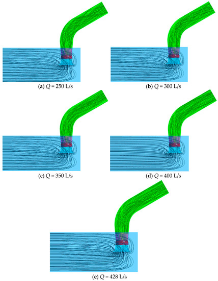
Figure 12.
A 3D flow distribution of the pump unit.
From Figure 12, it can be seen that the streamlines distribution of the open inlet channel under various flow conditions is relatively uniform. With the increase in flow, the streamlines located on both sides of the flare section converges toward the middle. The streamlines of the inlet channel along the inlet direction on the left and right sides are generally symmetrical with respect to the A3 surface. Under small flow conditions (Q = 250~350 L/s), the streamline inside the outlet bend is generally divided into two streamlines close to the inside and outside of the bend. The intertwining phenomenon of the internal streamlines is obvious, which is the main reason for the large hydraulic losses under this condition. With the increase in the flow rate, the uniformity of streamline distribution in the outlet channel of bend under design conditions (Q = 350 L/s) and large flow conditions (Q = 350~428 L/s) is improved; further, the best distribution is achieved at Q = 350 L/s.
5. Conclusions
In this study, the SST k-ω turbulence module is used to numerically assess an open inlet channel axial flow pumping rig according to the NS equation; moreover, the experimental energy characteristics are also verified. The main conclusions are as follows:
- (1)
- The test results suggest that the highest efficiency working conditions of the pump rig are Q1 = 333.27 L/s, head H1 = 6.718 m, efficiency η1 = 80.38%, the design working conditions are Q2 = 350 L/s, head H2 = 5.065 m, efficiency η2 = 79.56%, and the highest working head is H4 = 9.027 m (which is about 1.78 times that of the design head). Further, the pump rig can be said to have a wide range of operating conditions and the design conditions are within the designated high-efficiency operating conditions, therefore meeting the design requirements. The numerical calculation and test comparison error margins are within 5.0%, the numerical calculation and test measurement errors are small, and the numerical calculation results are credible.
- (2)
- The numerical calculation results demonstrate that the hydraulic loss of the inlet channel meets the relation hf = 0.5517Q2. Additionally, the hydraulic loss of the outlet bend meets the relation hf = 29.439Q2 − 22.27Q + 4.4992. Further, 80.675% of the inlet flow velocity uniformity of the pump unit’s impeller is in its design working condition (Q = 350 L/s), and 79.223% is in the weighted average angle of the flow velocity. As the flow increased, both the flow uniformity and the flow speed weighted average angle increased.
- (3)
- Through a comprehensive analysis of the flow patterns in the inlet channel, impeller, guide leaf, and outlet channel at different flow rates, it was found that the internal flow of the pump units is the most stable under the design condition Q = 350 L/s and, as a result, there are fewer bad flow patterns. The flow patterns of the inlet channel and outlet channel become worse when the flow rate decreases, and the flow pattern of the inlet channel is improved when the flow rate increases. However, compared with the design condition, the improvement is limited, and the flow pattern of the outlet channel is significantly worse.
Author Contributions
Concept design, C.X. and C.Z.; numerical calculations, T.F., A.F. and. T.Z.; experiments and data analysis, T.F., A.F., T.Z. and F.Y.; manuscript writing, C.X. and C.Z. All authors have read and agreed to the published version of the manuscript.
Funding
This research was funded by the Anhui Province Natural Science Funds for Youth Fund Project, grant number 2108085QE220. Funding was also provided by the Key scientific research project of Universities in Anhui Province, grant number KJ2020A0103; Anhui Province Postdoctoral Researchers’ Funding for Scientific Research Activities, grant number 2021B552; Anhui Agricultural University President’s Fund, grant number 2019zd10; and the Stabilization and Introduction of Talents in Anhui Agricultural University Research Grant Program, grant number rc412008.
Institutional Review Board Statement
Not applicable.
Informed Consent Statement
Not applicable.
Data Availability Statement
Not applicable.
Conflicts of Interest
The authors declare no conflict of interest.
References
- Qian, Y.; Yan, D.; Liu, C.; Cao, Z.; Jin, H. Experimental study on open inlet channels of pumping stations. J. Jiangsu Agric. Coll. 1989, 2, 47–52. [Google Scholar]
- Lu, L.; Xu, L.; Liang, J.; Liu, J.; Huang, J. Numerical calculation of three-dimensional flow and hydraulic loss in the inlet channel of pumping station. Drain. Irrig. Mach. 2008, 5, 55–58. [Google Scholar]
- Cheng, L.; Liu, C. Study on the objective function of optimal design of inlet and outlet water channels of pump stations. Water Pump Technol. 2007, 3, 39–42. [Google Scholar]
- Ye, P. Numerical Simulation and Experiments of Flow in Horn Pipe Inlet Channel of Axial Flow Pump. Master’s Thesis, Yangzhou University, Yangzhou, China, 2018. [Google Scholar]
- Qiu, C.; Zhang, Y. Simulation and analysis of the influence of the back wall distance of pumping station inlet basin on the water inlet conditions of pumps. Jiangsu Water Resour. 2012, 12, 17–18. [Google Scholar]
- Fu, J.; Li, N. Numerical optimization of pump station forebay and open intake channel. Jiangxi Sci. 2022, 40, 165–170. [Google Scholar]
- Sui, H. Study on the Hydraulic Optimization Design of Open Type Low Head Large Pumping Unit; Yangzhou University: Yangzhou, China, 2015. [Google Scholar]
- Zhang, W.; Shi, L.; Tang, F.; Duan, X.; Liu, H.; Sun, Z. Analysis of inlet flow passage conditions and their influence on the performance of an axial-flow pump. Proc. Inst. Mech. Eng. Part A J. Power Energy 2021, 235, 733–746. [Google Scholar] [CrossRef]
- Widodo, E.; Pradhana, R.Y. Analysis of pipe diameter variation in axial pumps for reducing head loss. In IOP Conference Series: Materials Science and Engineering; IOP Publishing: Bristol, UK, 2018; Volume 403. [Google Scholar]
- Yang, F.; Jiang, D.; Yuan, Y.; Lv, Y.; Jian, H.; Gao, H. Influence of Rotation Speed on Flow Field and Hydraulic Noise in the Conduit of a Vertical Axial-Flow Pump under Low Flow Rate Condition. Machines 2022, 10, 691. [Google Scholar] [CrossRef]
- Yang, F.; Li, Z.; Yuan, Y.; Liu, C.; Zhang, Y.; Jin, Y. Numerical and Experimental Investigation of Internal Flow Characteristics and Pressure Fluctuation in Inlet Passage of Axial Flow Pump under Deflection Flow Conditions. Energies 2021, 14, 5245. [Google Scholar] [CrossRef]
- Liu, X.; Xu, F.; Cheng, L.; Pan, W.; Jiao, W. Stress Characteristics Analysis of Vertical Bi-Directional Flow Channel Axial Pump Blades Based on Fluid–Structure Coupling. Machines 2022, 10, 368. [Google Scholar] [CrossRef]
- Pan, Q.; Zhao, R.; Wang, X.; Shi, W.; Zhang, D. LES study of transient behaviour and turbulent characteristics of free-surface and floor-attached vortices in pump sump. J. Hydraul. Res. 2019, 57, 733–743. [Google Scholar] [CrossRef]
- Park, I.; Kim, H.J.; Seong, H.; Rhee, D.S. Experimental Studies on Surface Vortex Mitigation Using the Floating Anti-Vortex Device in Sump Pumps. Water 2018, 10, 441. [Google Scholar] [CrossRef]
- Václav, U.; Pavel, P.; Milan, S.; Martin, K.; Daniel, D. Experimental and Numerical Study on Vortical Structures and Their Dynamics in a Pump Sump. Water 2022, 14, 2039. [Google Scholar]
- Shinichiro, Y. Numerical Study of the Vortical Structures in the Pump Sump. Proc. Fluids Eng. Conf. 2018, 2018, os15-11. [Google Scholar]
- Jiao, W.; Chen, H.; Cheng, L.; Zhang, B.; Yang, Y.; Luo, C. Experimental study on flow evolution and pressure fluctuation characteristics of the underwater suction vortex of water jet propulsion pump unit in shallow water. Ocean. Eng. 2022, 266, 112569. [Google Scholar] [CrossRef]
- Chen, X.; Wang, X.; Liu, Q. Numerical Study of Roll Wave Characteristics Based on Navier-Stokes Equations: A Two-Dimensional Simulation. J. Eng. Mech. 2021, 147, 04020149. [Google Scholar] [CrossRef]
- Alessandro, T.; Alberto, B.; Michele, C.; Gaetano, G.; Giorgio, M.; Francesca, S. Cfd simulations of early- to fully-turbulent conditions in unbaffled and baffled vessels stirred by a rushton turbine. Chem. Eng. Res. Des. 2021, 171, 36–47. [Google Scholar]
- Xie, C.; Zhang, C.; Fu, T.; Zhang, T.; Feng, A.; Jin, Y. Numerical Analysis and Model Test Verification of Energy and Cavitation Characteristics of Axial Flow Pumps. Water 2022, 14, 2853. [Google Scholar] [CrossRef]
- Madhu, B.P.; Mahendramani, G.; Bhaskar, K. Numerical analysis on flow properties in convergent—Divergent nozzle for different divergence angle. Mater. Today Proc. 2021, 45, 207–215. [Google Scholar] [CrossRef]
- Xie, C.; Feng, A.; Fu, T.; Zhang, C.; Zhang, T.; Yang, F. Analysis of Energy Characteristics and Internal Flow Field of “S” Shaped Airfoil Bidirectional Axial Flow Pump. Water 2022, 14, 2839. [Google Scholar] [CrossRef]
- Li, Y.; Zheng, Y.; Meng, F.; Osman, M.K. The Effect of Root Clearance on Mechanical Energy Dissipation for Axial Flow Pump Device Based on Entropy Production. Processes 2020, 8, 1506. [Google Scholar] [CrossRef]
- Stuparu, A.; Baya, A.; Bosioc, A.; Anton, L.; Mos, D. Experimental investigation of a pumping station from CET power plant Timisoara. In IOP Conference Series: Earth and Environmental Science; IOP Publishing: Bristol, UK, 2019; Volume 240. [Google Scholar]
- Xie, C.; Tang, F.; Yang, F.; Zhang, W.; Zhou, J.; Liu, H. Numerical simulation optimization of axial flow pump device for elbow inlet channel. In IOP Conference Series: Earth and Environmental Science; IOP Publishing: Bristol, UK, 2019; Volume 240. [Google Scholar]
- Sun, Z.; Yu, J.; Tang, F. The Influence of Bulb Position on Hydraulic Performance of Submersible Tubular Pump Device. J. Mar. Sci. Eng. 2021, 9, 831. [Google Scholar] [CrossRef]
- Ji, D.; Lu, W.; Lu, L.; Xu, L.; Liu, J.; Shi, W.; Huang, G. Study on the Comparison of the Hydraulic Performance and Pressure Pulsation Characteristics of a Shaft Front-Positioned and a Shaft Rear-Positioned Tubular Pump Devices. J. Mar. Sci. Eng. 2021, 10, 8. [Google Scholar] [CrossRef]
- Xie, C.; Xuan, W.; Feng, A.; Sun, F. Analysis of Hydraulic Performance and Flow Characteristics of Inlet and Outlet Channels of Integrated Pump Gate. Water 2022, 14, 2747. [Google Scholar] [CrossRef]
- Ahmed, N.; Yang, F.; Zhang, Y.; Wang, T.; Mahmoud, H. Analysis of the Flow Pattern and Flow Rectification Measures of the Side-Intake Forebay in a Multi-Unit Pumping Station. Water 2021, 13, 2025. [Google Scholar]
- Xie, C.; Fu, T.; Xuan, W.; Bai, C.; Wu, L. Optimization and Internal Flow Analysis of Inlet and Outlet Horn of Integrated Pump Gate. Processes 2022, 10, 1753. [Google Scholar] [CrossRef]
- Kan, K.; Zhang, Q.; Xu, Z.; Chen, H.; Zheng, Y.; Zhou, D.; Maxima, B. Study on a horizontal axial flow pump during runaway process with bidirectional operating conditions. Sci. Rep. 2021, 11, 21834. [Google Scholar] [CrossRef]
- Xie, C.; Yuan, Z.; Feng, A.; Wang, Z.; Wu, L. Energy Characteristics and Internal Flow Field Analysis of Centrifugal Prefabricated Pumping Station with Two Pumps in Operation. Water 2022, 14, 2705. [Google Scholar] [CrossRef]
- Zhang, W.; Tang, F.; Shi, L.; Hu, Q.; Zhou, Y. Effects of an Inlet Vortex on the Performance of an Axial-Flow Pump. Energies 2020, 13, 2854. [Google Scholar] [CrossRef]
- Yang, F.; Zhao, H.; Liu, C. Improvement of the Efficiency of the Axial-Flow Pump at Part Loads due to Installing Outlet Guide Vanes Mechanism. Math. Probl. Eng. 2016, 2016 Pt 2, 6375314. [Google Scholar] [CrossRef]
- Xie, C.; Zhang, T.; Yuan, Z.; Feng, A.; Wu, L. Optimization Design and Internal Flow Analysis of Prefabricated Barrel in Centrifugal Prefabricated Pumping Station with Double Pumps. Processes 2022, 10, 1877. [Google Scholar] [CrossRef]


Publisher’s Note: MDPI stays neutral with regard to jurisdictional claims in published maps and institutional affiliations. |
© 2022 by the authors. Licensee MDPI, Basel, Switzerland. This article is an open access article distributed under the terms and conditions of the Creative Commons Attribution (CC BY) license (https://creativecommons.org/licenses/by/4.0/).