Abstract
Discrete element simulation is an effective method to reveal the interaction between tillage components and work objects. However, due to the lack of discrete element modelling parameters of maize root and its mixture with soil, existing tillage models cannot accurately simulate the farmland environment under a no-tillage system. This study developed single maize root (SMR) with different diameters and maize root-soil mixture (MRSM) DEM models based on calibrated parameters through the angle of repose (AOR) tests. First, the Plackett–Burman and the steepest climb tests were performed to identify the range of essential parameters for the AOR of the SMR. Then, the optimal parameters for the SMR and MRSR models were obtained by Box–Behnken design (BBD) testing. The results showed that the static friction coefficient of SMR-SMR and the rolling friction coefficient of SMR-SMR and SMR-steel significantly affected the AOR. In addition, the AOR of MRSM was extremely sensitive to the restitution coefficient and surface energy coefficient of root soil. Based on optimal parameters, the relative errors between the simulated and measured AOR and pixel peak values of the piles’ contour curve were less than 5% for SMR and MRSM. The error of the dynamic AOR of the measured and simulated MSRM was less than 10%. These results indicate that the parameter calibration method and the developed models can be valuable references for DEM simulation for maize stubble and tillage.
1. Introduction
The maize root in farmland seriously affects the seedbed preparation and planting operations under a minimum or no-till system, including negatively affecting seed bed cleanliness and increasing the resistance of machinery [1,2,3,4,5,6]. Due to the lack of basic research on the interaction mechanism between crop roots and machinery, it is challenging to complete the selection, design, and optimization of tillage tools [7,8]. With modern computer technology improving constantly, simulation analysis has become an available method to understand the mechanical properties of soil and crops. Modeling the tillage process of a field with maize roots can effectively reveal the complex interaction between crop roots and machinery [9,10,11]. As a basis for the model, the accuracy of the maize root and root-soil mixture simulation guarantees the tillage model’s reliability.
The discrete element method (DEM) is a computer numerical simulation method based on the assumption of discontinuity, which has the advantages of saving time and effort, being low-cost, and enabling the visualization of results [12]. A discrete element simulation is completed based on rich particle contact models, such as the Hertz–Mindlin (no slip), Hertz–Mindlin with JKR, and Hertz–Mindlin with bonding model, etc. One critical step in developing a DEM model is determining the input parameters to describe the material and interaction properties of the particles [13,14,15]. These parameters mainly consist of intrinsic parameters and contact model parameters. The intrinsic parameters of materials can be obtained by tests directly, while contact model parameters are generally difficult to measure [3,4]. Therefore, it is necessary to calibrate the contact model parameters through simulation and physical experiments. Using various contact models, researchers have developed DEM models and calibrated parameters for agricultural materials, such as soil [16], seeds [17], crop straw [18], and fertilizers [19]. Wang et al., developed a DEM model of a citrus stalk with a diameter of 3 mm and conducted three-point bending and shear tests to complete the parameter calibration of the citrus stalk model [20]. Liao et al., simulated the angle of repose (AOR) and shearing failure test on the stalks from the harvest stage of feed rape using the DEM. The contact model parameters were calibrated by establishing the regression model of the AOR and shear force [21]. Ren et al., used the response surface method to optimize and calibrate the contact parameters of sugarcane leaves with the measured AOR as the response value [22]. Liu et al., determined the DEM parameters that significantly affected the AOR of adzuki beans with different materials based on the Plackett–Burman and steepest climbing tests and calibrated the critical factors by the Box–Behnken test [23]. Peng et al., chose the Hertz–Mindlin with JKR contact model to establish a DEM model of pig manure organic fertilizer to simulate the adhesion of material particles and calibrate the surface energy coefficient through the accumulation experiment [24]. Hu et al., calibrated the DEM parameters of coated delinted cotton seeds by combining the physical and simulation experiments based on the drum device [25]. Li et al., proposed a building method for the maize kernel model by rock DEM software and calibrated the model’s contact parameters through optimal experiments [26]. Additionally, Cao et al. [27], Ma et al. [28], and Liao et al. [29] calibrated the contact parameters of rapeseed, alfalfa stalks, and fodder rape particles by establishing a DEM model of the AOR test, respectively. These examples confirmed that the DEM can simulate a variety of agricultural materials with high accuracy. However, all existing study objects are mainly single materials, such as soil, seeds, straw, fertilizer, and others. There are few reports on the DEM simulation of the single maize root (SMR) and maize soil-root mixture (MRSM). With the continuous popularization of conservation tillage, it is necessary to build accurate and reliable DEM models for SMR and MRSM.
In this paper, the DEM model of SMR was developed using Discrete Element Modeling Expert (EDEM) based on the Hertz–Mindlin (no slip) contact model. The AOR tests of SMR, designed by Plackett–Burman, Slope-sliding, and Box–Behnken methods, were conducted to find and calibrate the parameters that significantly affected the AOR. On the basis of the SMR calibrated results, the MRSM DEM model was developed using the Hertz–Mindlin with JKR model. Its parameters were calibrated and optimized by the simulated BBD tests of AOR. Finally, the accuracy and reliability of the calibrated model were verified by comparing the actual and simulated values. The paper aims to provide a reference for the maize root and root-soil complex modeling approach, as well as the construction of the tillage DEM model.
2. Materials and Methods
2.1. Research Materials and Determination of Intrinsic Parameters
2.1.1. Research Materials
The maize variety Shaandan 609 was used as the research object. Ten maize stubble samples from different rows were randomly selected from the experimental field on the north campus of the Northwest A&F University in Yangling, Shaanxi, China. The maize ears were manually harvested in the fall of 2020, and the stubbles were maintained, waiting for the following spring sowing. Each stubble had nearly 60 SMR distributed in 2 to 4 layers (Figure 1a). Due to some SMR accompanied by varying structural damage, 16 SMR samples were collected through integrity screening. The SMR’s shape and structure were approximately cones. The root’s average length was 168.84 mm, and its diameter ranged from 1.0 to 5.0 mm, measured by a vernier caliper. An SMR was divided into four segments according to the diameter range to reduce the difficulty of the DEM model development and improve computational efficiency. The diameter range of each stage was 1–2, 2–3, 3–4, and 4–5 mm, marked as a, b, c, and d, respectively (Figure 1b). The average diameter and length of each segment was measured and counted, as shown in Table 1. To ensure the accuracy of the experimental data, all actual tests in this paper were completed within 72 h. The wet base moisture content of all single maize samples was between 22.78% and 35.60%.
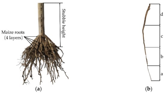
Figure 1.
The maize stubble (a) Root system of maize; and (b) SMR.

Table 1.
Segment length and diameter of an SMR.
2.1.2. Intrinsic Parameters of SMR
According to previous research results [1,3], the range of Poisson’s Ratio ν of SMR was 0.3–0.4 preliminarily. The volume and mass of SMR with different radii were measured using the drainage method and an electronic balance. The average density ρ of SMR was 266 kg/m3. The elastic modulus E of SMR was one of the critical parameters for establishing a DEM model, and its range can be determined by tensile tests [7]. As shown in Figure 2, the tensile testing equipment used the biomechanics testing machine with model DDL10 and EDC controller (Changchun Testing Machine Research Institute, Changchun, China). During the measurement, two ends of SMR were fixed vertically with a pair of clamps. The upper clamp stretched the SMR axially at a speed of 20 mm·min−1 until it was broken [30]. The elongation was obtained by measuring the distance between the unit gauge length points after a fracture. Due to the SMR with different diameters being similar to round bars, according to Hooke’s law, the relationship between stress σ and strain ε can be obtained as:
where Am is the effective cross-sectional area, F is the stress, Δl is the elongation, and l is the original gauge length. Since the average measured diameter of SMR mainly varied between 1.0 and 5.0 mm, the gauge lengths of the three styles were 20, 30, and 40 mm, respectively.
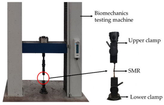
Figure 2.
Tensile test by a universal testing machine.
The average elastic modulus of an SMR in the four groups of diameters was 2.70 × 10⁸, 1.15 × 10⁸, 3.43 × 10⁷, and 2.30 × 10⁷ Pa; the average tensile strength was 30.3, 52.94, 94.56, and 118.88 N, respectively. The calculated relationship between material shear modulus G, elastic modulus E, and Poisson’s ratio is described by:
According to the determined range of Poisson’s Ratio ν, the shear modulus of a whole SMR ranged from 1.77 × 10⁷ to 2.08 × 10⁸ Pa, and its average was 8.51 × 10⁷ Pa.
2.1.3. Intrinsic Parameters of Soil
For the soil, loam soil developed on parent loess, collected from the same field as the SMR. The soil samples were collected within the depth of the maize root distribution using a ring knife. Referring to the method of Wang et al., the basic properties of soil samples were measured and counted as shown in Table 2 [31].
Table 2.
The basic properties of soil.
2.2. Preliminary DEM Model
2.2.1. Determine the Contact Model
A suitable contact model determines the reliability of the discrete element simulation. Due to the accurate and efficient force calculation of the Hertz–Mindlin contact model (HMCM), the SMR model was established as a combination of spherical particles based on HMCM using EDEM2020 (DEM Solutions, Edinburgh, UK) software [5,6,32]. Figure 3 illustrates the rationale of HMCM. It describes the force variation and energy loss by adding spring stiffness kt and kn, normal and tangential damping coefficients γn and γt, and the coefficient of friction μ when two particles come into contact. The contact force between particle i and j can describe the interaction of particles and be composed of the normal component and the tangential component [33,34].
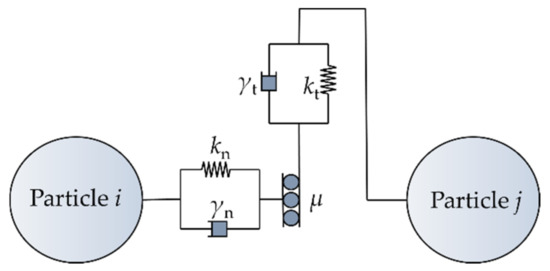
Figure 3.
Hertz–Mindlin contact model.
There is a phenomenon of adhesion between particles since the MRSM has a certain degree of humidity. In order to accurately simulate the adhesion between soil and roots, the simulation was performed using the Hertz–Mindlin with JKR (Johnson–Kendall–Roberts) contact model built in EDEM [35,36,37]. In this model, the normal elastic contact force FJKR is determined by the overlap δ, the interaction parameter, and the surface energy coefficient γ (Figure 4) based on the JKR theory [38], expressed as Equations (3)–(7):
where FJKR is the JKR normal elastic force, N; δ and α are the overlap and radius of two contact particles, respectively, m; and γ is the surface energy coefficient, N m−1. E* and R* were equivalent to Young’s modulus, pa, and radius, m, which can be determined using the following equations:
where ν1 and ν2 are Poisson’s Ratio of two particles; E1 and E2 are the shear modulus of two contact particles, Pa; and R1 and R2 are the radii of two contact particles, m.
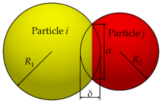
Figure 4.
Hertz–Mindlin with JKR contact model.
When γ is 0, FJKR is equal to the normal force in HMCM, which is calculated by the following equations:
2.2.2. Single Maize Root Model
To improve the computer processing speed in the simulation, the model in the current study was simplified, similar to most DEM simulations [1]. Since the AOR test simulation did not involve material bending or fracture, an approximate cylindrical multisphere composed of spheres in aggregation was established to describe the different parts of SMR. Figure 5 shows four SMR segments with different radii created for calibration experiments of contact parameters. The length of every SMR model is set to 15 mm to ensure the particles can fall smoothly in the AOR test [21].
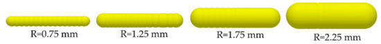
Figure 5.
Multisphere models of SMR with different radii.
2.3. Calibrated Experiments Design
2.3.1. Determine the Restitution Coefficient e
The restitution coefficient e describes the ability of an object to return to its original state after a collision. The freefall collision test was used to obtain the e range of the SMR-SMR, root-soil, and SMR-steel [6,10]. An SMR was prefabricated into four particle samples with an average diameter of 1.5, 2.5, 3.5, and 4.5 mm. These were allowed to fall freely at 200 mm and 400 mm onto the prepared plate. For the determination of SMR and the restitution coefficient between different materials, a steel plate, root rows, and soil plate were prepared as the base plate, respectively (Figure 6a). The process of SMR from falling to bouncing was recorded by an I-SPEED TR high-speed video camera (resolution: 2000 frames s−1) (OLYMPUS Co., Ltd., Tokyo, Japan). The highest rebound height was measured according to the captured frame after SMR collided with different materials (Figure 6b). The restitution coefficients are calculated by:
where H1 is the initial falling height of a single particle and H2 is the maximum height of contact rebound. After repeated experiments, the e of SMR-SMR, SMR-steel plate, and root-soil ranged from 0.01 to 0.1, 0.05 to 0.2, and 0.05–0.15, respectively.
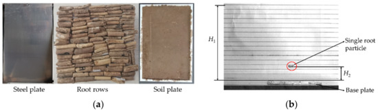
Figure 6.
Measurement of restitution coefficient e between SMR and different materials. (a) Base plate with steel, root, and soil; and (b) the freefalling and bouncing process of SMR.
2.3.2. Determine the Coefficient of Friction
Referring to the research methods of Liu et al., the slope-sliding test was used to determine the static friction coefficient μs range of SMR-SMR, SMR-steel, and root-soil. In order to ensure that the movement of SMR was only sliding on the slope, a number of them were bonded as a single sample [23]. Every sample was placed on the plate of the test bench as shown in Figure 7a. The distance between the initial position and bottom rotation axis was recorded as L1. The plate plane was raised slowly around the rotation axis until the sample slid on the plate. The height of the final position was measured as L2. The μs can be calculated by:
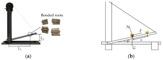
Figure 7.
Measurement of friction coefficient determination. (a) Static friction coefficient μs; and (b) Rolling friction coefficient μr.
When measuring the coefficient of rolling friction μr, the plate was slowly lifted until SMR started to move, and we recorded the angle φ between the horizontal plane and plate at this time [28]. When the rolling distance of SMR was s, the main forces on SMR included its gravity G, the supporting force from the measuring plane N, and the rolling friction force F (Figure 7b). According to the law of conservation of energy, the work done by the rolling friction of SMR during the rolling process Wr can be expressed by
where Ep is the initial gravitational potential energy of SMR, and Ek is the kinetic energy of SMR during the rolling process.
Since the quality of a sample was too small to precisely measure the final speed at the end of a certain rolling distance, this study assumed that the gravitational potential energy of SMR could be converted entirely into rolling friction work during short-distance rolling, that was, Ek = 0 [28]. μr can be calculated with Equation (11):
The experimental result showed that μs and μr of SMR-SMR ranged from 0.3 to 0.6 and 0.1 to 0.25; μs and μr of SMR-steel ranged from 0.3 to 0.5 and 0.1 to 0.25; and μs and μr of root-soil ranged from 0.45 to 0.65 and 0.15 to 0.25.
2.3.3. Determination of Actual Natural AOR
According to previous research on the AOR of plant stalks, the AOR test of SMR was carried out by the injection method shown in Figure 8a [28]. Before the measurement, SMR was prefabricated into four particle samples with a length of 15 mm and a diameter of 1.5, 2.5, 3.5, and 4.5 mm, respectively. Each sample with a mass of 2.5 g in equal proportions was mixed evenly. Then, the mixed SMR samples were poured into the funnel with an outlet (100 mm height × 25 mm inner diameter) and injected uniformly within 2 s. The AOR of the root pile was measured after all samples were stably piled on the receiving plate (300 mm length × 300 mm width). This experiment was repeated ten times, the average AOR θR of the SMR pile was 32.29 ± 0.8758°, and the coefficient of variation was 2.71% (Figure 8b).
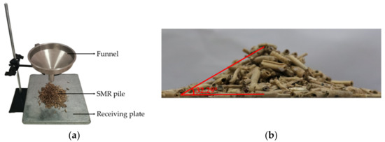
Figure 8.
Measurement of physical AOR of SMR. (a) Test device; and (b) AOR value.
The AOR of the MRSM was obtained by cylindrical lifting to calibrate the parameters based on a summary of related research [23,39]. The physical experimental device consists of a universal testing machine, a bottom plate (300 mm length × 300 mm width), and a steel cylinder (210 mm height × 70 mm inner diameter) (Figure 9a). Since the distribution depth of maize stubble ranges from 0 to 200 mm underground, the mass ratio of soil to root is 50:1 by separating the soil around the root system. Therefore, an MRSM consisting of soil (350 g) and SMR (7 g) was prepared, wherein the ratio in Table 1 determined the number of single roots with different diameters. The mixture was prepared and injected into the cylinder. Lifting the cylinder at a constant speed of 0.05 m·s−1 enabled the mixture to fall on the bottom plate through the lower end of the cylinder. The AOR on both sides was measured when the height of the pile no longer changed. This experiment was repeated ten times; the average AOR θM of the MRSM pile was 41.61 ± 1.29°, and the coefficient of variation was 3.55% (Figure 9b).
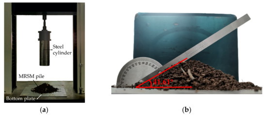
Figure 9.
Measurement of physical AOR of MRSM. (a) Test device; and (b) AOR value.
2.3.4. Simulation Model of the AOR Test
The discrete element models of AOR test for SMR and MRSM were developed using EDEM2020, respectively (Figure 10). For the SMR, a particle factory was created above the funnel, and four different diameters of SMR with a total amount of 12 g were generated dynamically at a speed of 6 g/s. The particles were given an initial velocity of 2 m/s to ensure the SMR fell rapidly and smoothly. When all the SMR particles were deposited on the bottom plate, the AOR of pile was measured and recorded by the protractor tool in the post-processing module. The total simulation test time was 6 s, and the Rayleigh time step was 2.3 × 10⁻⁶ s.
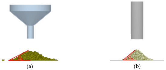
Figure 10.
The AOR simulation test of SMR and MRSM. (a) SMR; and (b) MRSM.
For the simulated AOR test of the MRSM, two particle factories were set up in the cylinder model to generate the same mass of SMR and soil particles as the physical test. According to the data in Table 1, the soil particle size conformed to a normal distribution within 3–7 mm and the length of the SMR model was set to 15 mm. To ensure the uniformity of mixing of soil and roots, the rotating cylinder method was utilized to realize the uniform MRSM. The cylinder was lifted upward at a steady rate of 0.05 m/s until the mixture accumulated on the bottom plate under the action of gravity. Based on the results of physical experiments and previous studies, the simulation parameter range between soil roots was determined [39]. The simulation parameter variation ranges in this study were determined as shown in Table 3.
Table 3.
Parameters of AOR simulation model for SMR and MRSM.
2.4. Design of AOR Simulation Test
2.4.1. AOR Simulation Test for SMR
To determine the optimal value of the significant parameter in the AOR test of SMR, the Plackett–Burman test was carried out by Design-Expert software (Stat-Ease, Minneapolis, MN, USA, V10.0.4). Firstly, the parameters with significant impact were screened out by comparing the relationship between the different levels of each factor and the target response value. Secondly, the steepest climbing test was carried out to determine the optimal value range of each significant parameter. The significant parameter gradually increased within its value range according to the fixed step length, while the non-significant factors took an intermediate level. The relative error η between simulated and physical test values was recorded as the target value. Finally, according to the design principle of Box–Behnken design (BBD), the high-level value, center point, and low-level value from the area adjacent to the optimal values were regarded as high (+1), medium (0), and low (−1) levels of significant parameters. In this test. The physical test results θR and η were used as the index, and the test results were analyzed by analysis of variance (ANOVA) to obtain the optimal solution.
2.4.2. AOR Simulation Test for MRSM
The BBD test was used to calibrate the parameters of the MRSM model. According to the range of the parameters (e, μs, μr, and γ) between the root and soil, each parameter had five levels coded as low (−1), middle (0), and high (+1) (Table 4). Based on the simulation results, a quadratic regression model was developed to describe the relationship between the angle of repose AOR and model parameters. Further, the optimal parameter combination of the MRSM model was determined by solving the regression equation.
Table 4.
Levels of factors for the BBD test of mixture AOR.
2.5. Validation Test of Dynamic AOR
To verify the accuracy and reliability of the calibrated parameters, the dynamic AOR of the MRSM was measured and simulated through a rotating drum test. The rotating drum test setup was similar to that used in a study by Adilet et al. [19]. As shown in Figure 11a, the inner diameter and thickness of the rotating steel drum were 150 and 50 mm, respectively. In order to observe and record the particle flow in the rotating drum, a plexiglass baffle was used on one side of the rotating drum. Through a speed governor, the stepper motor rotated the drum at a constant speed of 7.5 rpm. The mass ratio of soil to SR was 50:1, the total MSRM filling rate was 40%, and the total mass was 250 g, including equal amounts of SMRs with diameters of 1.5, 2.5, 3.5, and 4.5 mm, respectively. The flow images of MSRM particles in the rotating drum were captured by a camera, and 5 images were randomly selected to measure the dynamic AOR. The test setup of the simulation was consistent with the physical test (Figure 11b). The total simulation time was 10 s, and one particle flow image was captured at one-second intervals starting from the fourth second. According to the preformation of boundary extraction and linear fitting on the image, the slope of the straight line of the particle flow profile was obtained to calculate the dynamic AOR of MSRM.
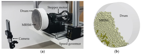
Figure 11.
The rotating drum test of MSRM. (a) Measurement; and (b) Simulation.
3. Results and Discussion
3.1. Calibration of Contact Parameters of SMR
3.1.1. The Result of the Plackett–Burman Test
The results of the Plackett–Burman test method are shown in Table 5. The contact parameters that affect the test results included x1–x8. The static friction coefficient of SMR-SMR x5, the rolling friction coefficient of SMR-SMR x7, and the rolling friction coefficient of SMR-steel plate x8 significantly affected simulated AOR through the ANOVA.
Table 5.
Significance ranking of contact parameters.
3.1.2. The Result of the Steepest Climbing Test
Six sets of simulated experiments for AOR were designed by expanding parameter values in the steepest climbing test (Table 6). It was determined that θR increased with the growth of factor levels, while the relative error η showed a trend of increasing first and then decreasing. The smallest relative error occurred in the third set of tests. It can be inferred that the optimal level range of three significant parameters was around it. Thus, the third group of parameter levels was taken as the center point (0) in the BBD test. The parameters of the second and fourth groups were taken as low (−1) and high (+1) levels for the simulated experiments.
Table 6.
The results of the steepest climbing test.
3.1.3. The Result of BBD Test
The Box–Behnken test result for AOR determined the optimal solution of significant parameters (Table 7). The quadratic polynomial of x5, x7, and x8 on the AOR (θR) was written as Equation (12) through multiple regression linear fitting.
Table 7.
Design matrix and results of the BBD test for the θR.
The results of ANOVA performed on the regression model of AOR are shown in Table 8. The p value of the model was less than 0.05, and the p value of the lack-of-fit term was greater than 0.05. The above data suggested that the model was extremely significant, and the equation had a high degree of fit. It also could be inferred that x5, x7, and x8 had highly significant effects on AOR. Additionally, the quadratic terms x5x7, x52, and x82 substantially impacted the AOR. In contrast, the x5x8, x7x8, and x72 had less impact on the AOR. Moreover, the determination coefficient R2 of the model was 0.9708, close to 1, indicating that the model can match the BBD test results well. The Adeq Precision result was 19.183 (Adeq Precision measures the signal-noise ratio, and a value greater than four is commonly required), which further means the model could predict the AOR of SMR truly and reliably.
Table 8.
ANOVA of the regression model of θR.
The quadratic regression Equation (12) was solved using the multi-objective optimization module in the Design Expert 10.0.4 software with the experimental value of AOR (32.29°) as the target value. The results of the optimal parameter combination (x5 = 0.371, x7 = 0.145, x8 = 0.212) were further selected from several parameter combinations as the best parameters through the minimization of η.
3.2. Calibration of Contact Parameters of MRSM
The BBD test results of MRSM are shown in Table 9. There were 29 groups of tests, which could be divided into two categories. One was the analysis points with a total of 24 groups; the other was the central points with 5 groups used to estimate the error of the experiment [1]. The second-order regression equation between the mixture AOR (θM) and the four parameters was performed by multivariate linear fitting analysis of test results using Design-Expert. According to the ANOVA results (Table 10), the equation excluding insignificant factors and items was written as:
Table 9.
Design matrix and results of the BBD test for θM.
Table 10.
ANOVA of the regression model of θM.
The ANOVA results showed that the p value of the regression model was less than 0.01, and the p value of the lack-of-fit term was greater than 0.05. It indicated that the model was significant in describing the relationship between the four parameters (x9, x10, x11, and x12) and θM. This model’s determination coefficient (R2) was 0.8467, indicating that the regression model was consistent with the BBD test results. Furthermore, the Adeq precision result reached 10.974, indicating that the obtained regression model can be used to predict the angle of repose of the mixture. According to the F value of the model, the influences of the four factors on θM were ranked in descending order: x12> x9> x10> x11. Among them, a, b, and c have a significant effect on θM; the other terms have no significant effect on the AOR of MRSM.
Response surfaces for each factor were investigated to further analyze the interaction with AOR in the two significant quadratic terms. Figure 12a shows that the response surface curve for the coefficient of rolling friction x12 is steeper than the restitution coefficient x10 of root-soil. It is demonstrated that x12 has a more significant effect on the AOR of MRSM; when the value of the x10 factor is constant, the AOR rapidly increases with the growth of x12. From Figure 12b, it can be seen that the response surface slope of the rolling friction coefficient is more significant relative to the static friction coefficient between soil roots, which further indicates that it has a more substantial impact on the AOR.
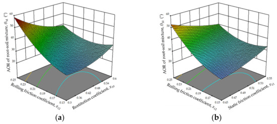
Figure 12.
Effects of interaction on the AOR of MRSM: (a) the interactive effects of the rolling friction coefficient and restitution coefficient of root-soil; and (b) the interactive effects of the rolling friction coefficient and static friction coefficient of root-soil.
Within the range of factor levels, the parameters were optimized by the optimization module of the Design-Expert software. The physical AOR (41.61°) of MRSM was the optimization target value, and x9, x10, x11, and x12 were regarded as the optimization objects. The following optimal combinations of the factors were obtained: the static and rolling friction coefficients of root-soil were 0.45 and 0.23, respectively, the restitution coefficient of root-soil was 0.41, and the surface energy coefficient of root-soil was 3.33 J·m−2.
3.3. Validation Tests
The AOR of SMR and MRSM in simulations based on the optimized parameter combinations were carried out, respectively. From Figure 13, the average value of simulated AOR on SMR and MRSM was 32.18° and 40.71°. An independent sample t-test was performed on the simulated and physical test values. For the SMR, the results showed Pt = 0.761 > 0.05, and the relative error was 0.34%, indicating the calibrated model can accurately simulate the AOR of SMR. For the MRSM, the results showed Pt = 0.181 > 0.05, and the relative error between the simulated and measured AOR was 0.22%, indicating that the DEM parameters of MRSM were reliable.
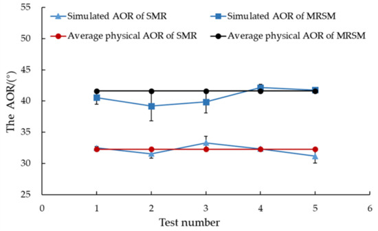
Figure 13.
Comparison between the average physical and the simulation value of the AOR under the optimal parameter combination.
The edge detection method of the Canny Operator was used to extract the contour of the material pile in the experiment and simulation experiment. The contour fit curve exactly showed the difference between the model and the actual value. This method not only considers the AOR of the material but also quantitatively compares the material pile as a whole structure, which further verifies the accuracy of the calibration results. The contours of the original stack were extracted through gray-scaled treatment, and boundary extraction was conducted using Python based on the Canny operator algorithm (Figure 14). Figure 15a compares the simulated and physical contour of the SMR pile. The pixel distribution of the three curves was consistent with the actual image, and the coincidence of the simulated test and the actual test profile curve after calibration is higher than before. Via fitting the contour curve with Gaussian distribution, the three curves’ vertical pixel peak serves were 204.218, 164.048, and 171.472, respectively (Figure 15b). The pixel peak error of the simulation test after calibration and the actual test was 4.33%. It further showed that the calibrated contact parameters effectively improved the reliability of the AOR test model.
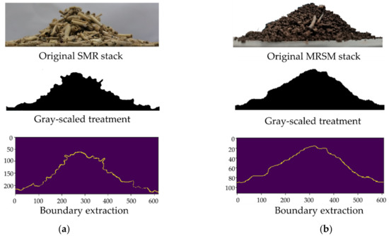
Figure 14.
The contour extraction process of the stack of SMR (a), and MRSM (b).
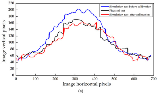
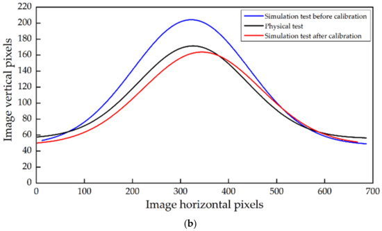
Figure 15.
Comparison of the simulated and actual SMR stack. (a) Contour comparison; and (b) fitted curve comparison.
Contour extraction and curve fitting were conducted on the MRSM pile utilizing the same method used in the SMR (Figure 16). The vertical pixel peaks of the calibration model, the uncalibrated model, and the actual test contour fitting curve were 116.96, 174.59, and 122.05, respectively. The peak error of the curve between the calibration model and the actual test was 4.17%, indicating that the developed model could better simulate the actual AOR for the soil root mixture.
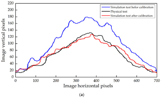
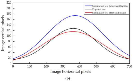
Figure 16.
Comparison of the simulated and actual MRSM stack. (a) Contour comparison; and (b) Fitted curve comparison.
Figure 17a,b shows the measured and simulated accumulation layer of MSRM at a certain moment. By comparing the dynamic AOR at different times when the drum rotational speed was 7.5 rpm, the relative errors between the simulated and actual tests at each moment were less than 10%, and all were within the error range of the test results (Table 11). The simulated dynamic AOR was generally larger than the measured value, which can be attributed to the inevitable gaps between rigid soil particles. However, in the actual situation, the gap between soil particles was minimal with tighter contact so that the free slope of the accumulation layer was not as steep as the simulation results. Furthermore, root-soil agglomeration was observed in the drum due to the adhesion between SMR and soil (Figure 17c,d). The simulation observed a consistent phenomenon with measurement, proving that the JKR model can accurately reflect the cohesion between particles. The drum test results show that the developed model can simulate the material properties of MRSM well.
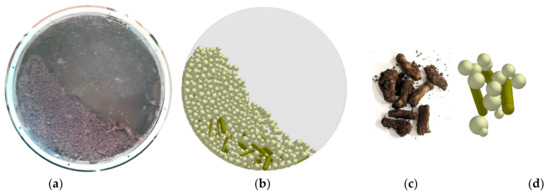
Figure 17.
Accumulation layer of MSRM and Soil-Root aggregation in measured (a,c) and simulated (b,d) drum tests.
Table 11.
Results of rotating drum test for MRSM.
In summary, the simulation test results based on the calibrated significant parameters show good agreement with the physical test results. Therefore, the above results can be used for simulation in future soil tillage studies. However, it should be noted that when the root shape and soil properties change, the parameters need to be further calibrated to bring the simulation closer to the actual test and enhance the practical significance of the simulation.
4. Conclusions
This study aimed to calibrate the DEM parameters of SMR and MRSM as the basis for tillage simulation under conservation agriculture models. Combined with physical and simulation experiments, the significant parameters of the SMR and its interaction with soil were measured, calibrated, and verified by AOR tests. The freefall collision and slope-sliding tests determined the contact parameter ranges of the SMR. Three significant parameters, the static friction coefficient, rolling friction coefficient of SMR-SMR, and rolling friction coefficient of SMR-steel were 0.341, 0.145, and 0.212, and were calibrated by solving the regression equation of AOR, respectively. For the MRSM, the optimal combination of the parameters was obtained as the static and rolling friction coefficients of root-soil were 0.45 and 0.23, respectively, the restitution coefficient of root-soil was 0.41, and the surface energy coefficient of root-soil was 3.33 J·m−2. The validation test illustrated that the relative errors between the simulated and measured AOR values of SMR and MRSM were 0.34% and 0.22%, respectively. Meanwhile, the relative errors between simulated and measured pixel peak values of the stacking contour fitting curve were 4.33% and 4.17%, respectively. The relative error between the simulation and the measured dynamic AOR was less than 10%, and the JKR contact model was used to simulate the soil-root adhesion in the rotating drum test accurately. All the results showed that the calibration method used in this study is feasible, and the calibrated parameters of SMR and MRSM can be utilized further to simulate maize stubble and operation environment of no-tillage. It is noted that the simulations and actual experiments were performed under a given maize variety and soil condition. Caution should be taken when using the optimization results for different situations.
Author Contributions
Conceptualization, S.Z.; methodology, S.Z.; software, J.D.; validation, X.C.; formal analysis, F.Y.; investigation, Y.L.; resources, G.M.; data curation, X.J.; writing—original draft preparation, S.Z.; writing—review and editing, X.W.; visualization, T.W.; supervision, Y.H.; project administration, Y.H.; funding acquisition, Y.H. All authors have read and agreed to the published version of the manuscript.
Funding
This research was funded by The National Key Research and Development Program of China (grant number: 2021YFD2000405); Science & Technology Program of Henan Province (grant number: 222102110456).
Institutional Review Board Statement
Not applicable.
Informed Consent Statement
Not applicable.
Data Availability Statement
Not applicable.
Conflicts of Interest
The authors declare no conflict of interest.
References
- Niu, M.; Fang, H.; Chandio, F.; Shi, S.; Xue, Y.; Liu, H. Design and experiment of separating-guiding anti-blocking mechanism for no-tillage maize planter. Trans. CSAE 2019, 50, 52–58. [Google Scholar]
- Zeng, Z.W.; Thoms, D.; Chen, Y.; Ma, X. Comparison of soil and corn residue cutting performance of different discs used for vertical tillage. Sci. Rep. 2021, 11, 2537. [Google Scholar] [CrossRef] [PubMed]
- Aikins, K.A.; Ucgul, M.; Barr, J.B.; Jensen, T.A.; Antille, D.L.; Desbiolles, J.M.A. Determination of discrete element model parameters for a cohesive soil and validation through narrow point opener performance analysis. Soil Tillage Res. 2021, 213, 105123. [Google Scholar] [CrossRef]
- Adajar, J.B.; Alfaro, M.; Chen, Y.; Zeng, Z.W. Calibration of discrete element parameters of crop residues and their interfaces with soil. Comput. Electron. Agric. 2021, 188, 11. [Google Scholar] [CrossRef]
- Zhao, H.; Li, H.; Ma, S.; He, J.; Wang, Q.; Lu, C.; Zhang, C. The effect of various edge-curve types of plain-straight blades for strip tillage seeding on torque and soil disturbance using DEM. Soil Tillage Res. 2020, 202, 104674. [Google Scholar] [CrossRef]
- Eden, M.; Bachmann, J.; Cavalaris, C.; Kostopoulou, S.; Kozaiti, M.; Boettcher, J. Soil structure of a clay loam as affected by long-term tillage and residue management. Soil Tillage Res. 2020, 204, 104734. [Google Scholar] [CrossRef]
- Fang, M.; Yu, Z.H.; Zhang, W.J.; Cao, J.; Liu, W.H. Friction coefficient calibration of corn stalk particle mixtures using Plackett-Burman design and response surface methodology. Powder Technol. 2022, 396, 731–742. [Google Scholar] [CrossRef]
- Qin, K.; Cao, C.M.; Liao, Y.; Wang, C.; Fang, L.; Ge, J. Design and optimization of crushing and throwing device for straw returning to field and fertilizing hill-seeding machine. Trans. CSAE 2020, 36, 1–10. [Google Scholar]
- Du, J.; Heng, Y.F.; Zheng, K.; Luo, C.M.; Zhu, Y.H.; Zhang, J.M.; Xia, J.F. Investigation of the burial and mixing performance of a rotary tiller using discrete element method. Soil Tillage Res. 2022, 220, 17. [Google Scholar] [CrossRef]
- Zhang, T.; Liu, F.; Zhao, M.; Liu, Y.; Li, F.; Chen, C.; Zhang, Y. Movement law of maize population in seeds room of seeds metering device based on discrete element method. Trans. Chin. Soc. Agric. Eng. 2016, 32, 27–35. [Google Scholar]
- Wang, X.Z.; Gao, P.Y.; Yue, B.; Shen, H.; Fu, Z.L.; Zheng, Z.Q.; Zhu, R.X.; Huang, Y.X. Optimisation of installation parameters of subsoiler’ wing using the discrete element method. Comput. Electron. Agric. 2019, 162, 523–530. [Google Scholar] [CrossRef]
- Cundall, P.A.; Strack, O. A discrete numerical model for granular assemblies. Géotechnique 2008, 30, 331–336. [Google Scholar] [CrossRef]
- Ucgul, M.; Fielke, J.M.; Saunders, C. 3D DEM tillage simulation: Validation of a hysteretic spring (plastic) contact model for a sweep tool operating in a cohesionless soil. Soil Tillage Res. 2014, 144, 220–227. [Google Scholar] [CrossRef]
- Horabik, J.; Molenda, M. Parameters and contact models for DEM simulations of agricultural granular materials: A review. Biosyst. Eng. 2016, 147, 206–225. [Google Scholar] [CrossRef]
- Coetzee, C.J. Calibration of the discrete element method. Powder Technol. 2017, 310, 104–142. [Google Scholar] [CrossRef]
- Ucgul, M.; Fielke, J.M.; Saunders, C. Three-dimensional discrete element modelling of tillage: Determination of a suitable contact model and parameters for a cohesionless soil. Biosyst. Eng. 2014, 121, 105–117. [Google Scholar] [CrossRef]
- Chen, Z.; Wassgren, C.; Veikle, E.; Ambrose, K. Determination of material and interaction properties of maize and wheat kernels for DEM simulation. Biosyst. Eng. 2020, 195, 208–226. [Google Scholar] [CrossRef]
- Liu, F.; Zhang, J.; Chen, J. Modeling of flexible wheat straw by discrete element method and its parameters calibration. Int. J. Agric. Biol. Eng. 2018, 11, 42–46. [Google Scholar] [CrossRef]
- Adilet, S.; Zhao, J.; Sayakhat, N.; Chen, J.; Nikolay, Z.; Bu, L.; Sugirbayeva, Z.; Hu, G.; Marat, M.; Wang, Z. Calibration Strategy to Determine the Interaction Properties of Fertilizer Particles Using Two Laboratory Tests and DEM. Agriculture 2021, 11, 592. [Google Scholar] [CrossRef]
- Wang, Y.; Zhang, Y.; Yang, Y.; Zhao, H.; Yang, C.; He, Y.; Xu, H. Discrete element modelling of citrus fruit stalks and its verification. Biosyst. Eng. 2020, 200, 400–414. [Google Scholar] [CrossRef]
- Liao, Y.; Liao, Q.; Zhou, Y.; Wang, Z.; Jiang, Y.; Liang, F. Parameters calibration of discrete element Model of fodder rape crop harvest in bolting Stage. Trans. CSAE 2020, 51, 73–82. [Google Scholar]
- Ren, J.H.; Wu, T.; Mo, W.Y.J.; Li, K.; Hu, P.; Xu, F.Y.; Liu, Q.T. Discrete element simulation modeling method and parameters calibration of sugarcane leaves. Agronomy 2022, 12, 1796. [Google Scholar] [CrossRef]
- Liu, Y.; Mi, G.P.; Zhang, S.L.; Li, P.; Huang, Y.X. Determination of discrete element modeling parameters of adzuki bean seeds. Agriculture 2022, 12, 13. [Google Scholar]
- Peng, C.; Xu, D.; He, X.; Tang, Y.; Sun, S. Parameter calibration of discrete element simulation model for pig manure organic fertilizer treated with Hermetia illucen. Trans. CSAE 2020, 36, 212–218. [Google Scholar]
- Hu, M.J.; Xia, J.F.; Zhou, Y.; Luo, C.M.; Zhou, M.K.; Liu, Z.Y. Measurement and calibration of the discrete element parameters of coated delinted cotton seeds. Agriculture 2022, 12, 286. [Google Scholar] [CrossRef]
- Li, H.C.; Zeng, R.; Niu, Z.Y.; Zhang, J.Q. A calibration method for contact parameters of maize kernels based on the discrete element method. Agriculture 2022, 12, 664. [Google Scholar] [CrossRef]
- Cao, X.L.; Li, H.; Li, H.W.; Wang, X.C.; Ma, X. Measurement and calibration of the parameters for discrete element method modeling of rapeseed. Processes 2021, 9, 605. [Google Scholar] [CrossRef]
- Ma, Y.; Song, C.; Xuan, C.; Wang, H.; Yang, S.; Wu, P. Parameters calibration of discrete element model for alfalfa straw compression simulation. Trans. CSAE 2020, 36, 22–30. [Google Scholar]
- Liao, Y.; Wang, Z.; Liao, Q.; Wan, X.; Zhou, Y.; Liang, F. Calibration of discrete element model parameters of forage rape stalk at early pod stage. Trans. CSAM 2020, 51, 236–243. [Google Scholar]
- Xu, Y.F.; Zhang, X.L.; Sun, X.J.; Wang, J.Z.; Liu, J.Z.; Li, Z.G.; Li, P.P. Tensile mechanical properties of greenhouse cucumber cane. Int. J. Agric. Biol. Eng. 2016, 9, 1–8. [Google Scholar]
- Wang, X.; Zhang, S.; Pan, H.; Zheng, Z.; Huang, Y.; Zhu, R.X. Effect of soil particle size on soil-subsoiler interactions using the discrete element method simulations. Biosyst. Eng. 2019, 182, 138–150. [Google Scholar] [CrossRef]
- EDEM. EDEM Tutorial: Flexible Plane Simulation; DEM Solutions: Edinburgh, UK, 2020. [Google Scholar]
- Guo, Y.; Chen, Q.; Xia, Y.; Westover, T.; Eksioglu, S.; Roni, M. Discrete element modeling of switchgrass particles under compression and rotational shear. Biomass Bioenergy 2020, 141, 105649. [Google Scholar] [CrossRef]
- Guo, J.; Karkee, M.; Yang, Z.; Fu, H.; Li, J.; Jiang, Y.L.; Jiang, T.T.; Liu, E.X.; Duan, J.L. Discrete element modeling and physical experiment research on the biomechanical properties of banana bunch stalk for postharvest machine development. Comput. Electron. Agric. 2021, 188, 31. [Google Scholar] [CrossRef]
- Roessler, T.; Katterfeld, A. DEM parameter calibration of cohesive bulk materials using a simple angle of repose test. Particuology 2019, 45, 105–115. [Google Scholar] [CrossRef]
- Yano, T.; Ohsaki, S.; Nakamura, H.; Watano, S. Numerical study on compression processes of cohesive bimodal particles and their packing structure. Adv. Powder Technol. 2021, 32, 1362–1368. [Google Scholar] [CrossRef]
- Hoshishima, C.; Ohsaki, S.; Nakamura, H.; Watano, S. Parameter calibration of discrete element method modelling for cohesive and non-spherical particles of powder. Powder Technol. 2021, 386, 199–208. [Google Scholar] [CrossRef]
- Johnson, K.L.; Kendall, K.; Roberts, A. Surface energy and the contact of elastic solids. Proc. R. Soc. Lond. A Math. Phys. Sci. 1971, 324, 301–313. [Google Scholar]
- Tian, X.L.; Cong, X.; Qi, J.T.; Guo, H.; Li, M.; Fan, X.H. Parameter calibration of discrete element model for corn straw-soil mixture in black soil areas. Trans. CSAE 2021, 52, 100–108+242. [Google Scholar]


Publisher’s Note: MDPI stays neutral with regard to jurisdictional claims in published maps and institutional affiliations. |
© 2022 by the authors. Licensee MDPI, Basel, Switzerland. This article is an open access article distributed under the terms and conditions of the Creative Commons Attribution (CC BY) license (https://creativecommons.org/licenses/by/4.0/).