Abstract
In this study, we propose a hypocenter localization algorithm that uses the time difference of arrival (TDOA) and angle of arrival (AOA) as a hybrid model. The hypocenter measurements are detected by the accelerator sensors of the four separate observatories that are closest to the origin of an earthquake. The measurements are calibrated by the proposed deep learning P-onset picking system with short-time Fourier transform (STFT) signal analysis because the accurate detection of Primary waves (P-waves) is limited by seismic environmental noise. The revised measurements are used to calculate the precise distances between the observatories and hypocenters. The proposed hybrid TDOA/AOA is represented by a linear matrix equation that includes the unknowns of the precise distances, coordinates, and arrival angles to the observatories. We estimate a hypocenter using the constrained least squares method (CLS) under the constraints of the TDOA/AOA. The objective function with the constraints is optimized using the Lagrange function, and the asymptotic optimum is obtained by specifying the optimal Lagrange multipliers. Simulations show the performance of the proposed hypocenter localization method.
1. Introduction
Hypocenter localization is one of the most significant issues in seismic monitoring systems such as earthquake early warning systems and urgent earthquake detection and alarm systems [1,2]. The precise estimation of an earthquake location enables the quantification of the scale of the hazard, the casualty rescue, and future hazard forecasting. Seismic events occur when kinetic energy is briefly released by tectonic activity within a short period of 1–3 min. Thus, rapid estimation is important for the prompt prevention of earthquake hazards. Seismic waves originating from the hypocenter first affect the vertically located epicenter and then spread in a similar manner to the water surface on the Earth’s crust because the kinetic energy of the earthquake is transferred omnidirectionally from the hypocenter. Accordingly, seismic signals are sequentially detected by accelerator sensors in observatories on the surface of the Earth’s crust. These waves are categorized as first arrival waves, which are the primary waves (P-waves), and destructive waves, which are the secondary waves (S-waves). By analyzing and researching the detected seismic waveforms, earthquake monitoring systems’ precision and rapid prevention can be improved.
In seismology, the epicenter or hypocenter is located by multiple seismic stations. At different locations, the stations record seismic waves using seismograms and offer information to the corresponding seismic network to estimate the distances between the earthquake and observatories. Based on the seismic waves, the distances are estimated from the difference between the P- and S-wave arrival times. The curves of the P- and S-wave travel times are used to calculate the distances with the time difference and have been utilized in many studies including recent reports [3,4]. The fastest manner of detecting P-waves is to select the time of the P-onset. Based on the superiority of this method, the seismic distance estimation method using P-onset picking and the propagation speed of P-waves has been extensively studied [5,6,7]. To identify the P-onset, conventional methods such as short- and long-term averaging, calculating the skewness and kurtosis of seismic waves, and various other methods have been used. Nevertheless, determining the P-onset is difficult because seismic waves include environmental noise. Recently, owing to the remarkable feature extraction ability of state-of-the-art deep learning technologies (DLT), many achievements have been made in computer vision, signal processing, and other classification problems. Engineering issues have been solved, and meaningful research has been conducted on the P-onset picking issue using DLT, which can identify and learn complex patterns in seismic data [8,9,10,11,12].
For many years, in the fields of wireless communication, device-free localization, mobile networks, and the Internet of Things, the time difference of arrival (TDOA) and angle of arrival (AOA) methods were the primary methods for emitter positioning [13,14]. Based on the location of the receivers, the TDOA method can be represented by a linear algebraic equation with the distances between the emitter and receivers. The signals recorded on the receivers have a velocity that contributes to reliably specifying the exact location of the emitter using sequentially arriving signals. However, the TDOA exhibits a limited performance under deteriorated geometrical conditions. To address this problem, the AOA method can be applied to 3D localization. The AOA is the main method used in active radio-source localization processes [15]. In the AOA method, an emitter generates information of two angles that represent the horizontal and vertical properties of receiver stations. Based on the horizontal and vertical angles, the AOA method can be expressed as a linear algebraic equation. The TDOA/AOA method can specify a more accurate position of the emitter by reducing the emitter signal noise. Because the TDOA and AOA measurement errors are uncorrelated, a hybrid technique can be applied to leverage both localization methods. A hybrid technique has been proposed to efficiently concatenate the available information [16,17]. The advantages of the hybrid method are more significant in situations with limited receivers or unreliable signals. In seismic localization, the location of an earthquake is determined using the geometrical trilateration method. However, this method cannot specify the location when the reported seismic distances are under- or overestimated. Using the least squares method (LS), the earthquake location is simply specified by one coordinate solution [18]. Because the hybrid TDOA/AOA models need to satisfy two constraints, a more precise solution can be estimated using constrained least squares (CLS) to approximate the objective target with a Lagrange multiplier and function [19].
In the seismic geolocation field, the estimation accuracy of an earthquake’s location is one of the most challenging and important issues. Under real circumstances, the estimated location is not always accurate because the signals detected contain environmental and measurement sensor noise. Many efforts have been made to predict earthquake location precisely. Zhang [20] proposed a forward-transmission laser interferometry method using a widely distributed optical fiber link. Using the fiber network, the epicenter was precisely located using a geometric method. Lee [21] presented an epicenter location estimation using a laser-interferometry seismometer with LS. Seismic signals were analyzed using a high-precision instrument and short-time Fourier transform (STFT) for the specification of seismic signal properties. Gasparini [22] suggested a real-time hypocenter localization method for early warning systems based on an equal differential time and probabilistic approach. Zhu [23] proposed an estimation algorithm for epicenter location using a frequency domain that can estimate faster than the time domain.
The techniques introduced in [20,21,22,23] are compared as shown in Table 1 in terms of the instrument, the material, the signal property extraction, the localization modeling method, the state-of-the-art application, the estimation algorithm, and the estimation solution. The techniques can be improved using the TDOA/AOA CLS method with calibrated P-onset distances that have high certainty. The proposed method does not require high-precision instruments or high-quality materials over a wide range. The proposed seismic accelerometer sensor network can be simply applied by analyzing the seismic signals with extremely accurate precision. The seismic waves are analyzed as spectogram images by STFT to discriminate the seismic data characteristics. Furthermore, the proposed hypocenter localization method can specify the single solution coordinate of an earthquake location in three dimensions as the hypocenter. In the case where there are multiple samples, which are the solution coordinates by CLS, the proposed strategy can be evaluated by various methods. However, this study introduces 10 samples of hypocenter estimation because the proposed hypocenter localization procedure takes several preprocesses. In the field of localization, the Cramer–Rao lower bound has been used to verify the performance of the estimation method and has also been demonstrated as a reference [24]. In [24], we can also confirm that the root mean square error of the CLS-based estimation was smaller than that of the LS-based estimation for the same standard deviation in the mobile network problem. Owing to its many advantages, the hybrid TDOA/AOA CLS method was applied for hypocenter localization in this study. Moreover, since there has been no study on the hybrid technique for seismic localization, this study presents the process of applying the hybrid TDOA/AOA method to hypocenter localization together with the DLT. Each linear equation of the TDOA and AOA was concatenated into one hybrid linear equation, and the Lagrange function with two constraints was set as the objective function. Since the number of variables in the constraint was more than two, and there were two constraints, we adopted the Lagrange multiplier method as a solution for constrained optimization. Because of the two constraints, the two Lagrange multipliers were asymptotically approximated by gradient descent using the Jacobian matrix of the Lagrange function. The optimal Lagrange multiplier allows the solution of the CLS to estimate the hypocenters more precisely.

Table 1.
Comparison of the related literature.
In addition, we describe a method for estimating the correct P-onset. Seismic waves are complex signals comprising P-waves, S-waves, and natural noise elements. The P-wave is the signal that has the most prominent kinetic energy before the S-wave arrives. Using the characteristics of the P-wave, the point at which the amplitude of the seismic wave suddenly increases for the first time can be defined as the P-onset. A specific amplitude value can be designated as a threshold, and the first point in the seismic wave that exceeds the threshold can be determined as the P-onset. However, although the threshold method is ideal for signals in which only P- and S-waves exist, it may over- or underestimate the P-onset in seismic signals with added natural noise. Therefore, we analyzed the seismic signals using the STFT to extract new signal features. The signal features extracted by the STFT were used to determine the P-onset by distinguishing the noise from the important information in the seismic signals.
In this study, we selected the P-onset using binary classification between the noise and P-waves using DLT, particularly GoogLeNet [25]. In addition, our deep learning model required a 10-s (i.e., approximately 5 s before and 5 s after the P-wave arrival time) seismic waveform as the format of the dataset. The dataset consisted of spectrogram images characterized by the STFT of the noise and P-wave signals. Consequently, we reconfigured our deep learning model as a binary classifier using the GoogLeNet structure and then trained the model on the spectrogram image dataset labeled with noise and P-waves. After performing spectrogram image processing on seismic waves that had three components at four stations, the P-wave probability was estimated using the pretrained deep learning model, and we determined the highest probability point of the P-wave as a P-onset. We compensated for the reported distances of real circumstances for the P-onset revised distances using the results of the trained model.
The remainder of this paper is organized as follows. Section 2 explains the localization system model based on the hybrid TDOA/AOA. Section 3 presents the CLS with the hybrid TDOA/AOA model. The performance of the proposed method is demonstrated in Section 4 through simulation results in a real environment. Finally, Section 5 provides the conclusions.
2. Hybrid TDOA/AOA Modeling for the Hypocenter
In this section, we explain the estimation algorithms of the TDOA and AOA models. We then analyze the hybrid TDOA/AOA localization model to obtain the hypocenter based on the CLS algorithm for the first time in seismic localization fields. The TDOA localization method is a technique for estimating the location of a target using the arrival time difference of a signal. The AOA localization provides location information using the difference in signal reception angles in the three base stations that received a signal from a hypocenter. By combining these two methods, we developed a hybrid TDOA/AOA model for hypocenter localization. The limited vertical estimation performance of the 3D TDOA was overcome by the AOA, and the horizontal estimation performance of the AOA was supplemented by the TDOA. Therefore, combining the TDOA and AOA improved the location estimation performance because the technologies complement each other.
In Figure 1, represents the observatory location. In addition, is the distance between the hypocenter and the i-th station in 3D, and is the distance between the hypocenter and the i-th station on the x-y plane. denotes the angle between the hypocenter and the i-th observatory with respect to the z-axis, and denotes the angle between the hypocenter and the i-th observatory with respect to the y-axis. The modeling for TDOA/AOA localization utilizes , , , and , which were observed at each station. From these variables, we represent the TDOA and AOA in a matrix form or matrix equation. We then combine the TDOA and AOA equations and propose the localization method using CLS in Section 2.1–Section 3.
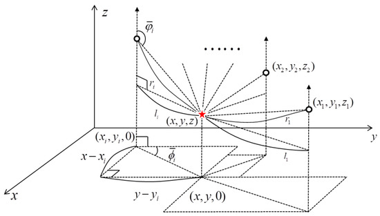
Figure 1.
Hypocenter localization using distance and angle.
2.1. TDOA Modeling
The main idea in Section 2 is to determine the hypocenter using an algorithm that applies both TDOA and AOA. In this section, based on Figure 1, we analyze the TDOA localization. Several approaches have been used on the signal originating from the receiver of the observatory based on TDOA [13,14]. We assume that the hypocenter is at , and the i-th receiver is at , . Then, we can express the equation for the distance r as follows:
where is the difference between and , is the distance between the hypocenter and the i-th receiver, is the distance between the hypocenter and first receiver, c is the signal propagation speed of the P-wave, and is the TDOA value. We can then rewrite as follows [26]:
By including the noise factor, Equation (2) can be obtained. After rearranging Equation (2), we obtain the following expression by squaring both sides. Therefore, the closed form of the TDOA relation can be expressed as follows:
Without much difficulty, the solution to Equation (3) in a matrix equation can be calculated, even if the number of observations increases. Because the data obtained in the real environment include noise, we define as noise. By including the noise factor, Equation (4) can be obtained. Equation (3) can be rewritten in the following matrix form:
is the ideal TDOA matrix that is free of noise factors. In Equation (5), the location of the reference receiver is set as , and the solution of the hypocenter localization represents . In addition, N denotes the number of observatories, which must be at least three and typically greater than four. In real cases, the TDOA parameter is substituted by the measurement value that contains the measurement error. Therefore, as in Equation (3), noise is added to the matrix.
2.2. Hybrid TDOA/AOA Modeling
The next step is to derive an expression for AOA localization. The angles of and shown in Figure 1 must be measured between the hypocenter and observatories. The distance between the emitter and the i-th receiver on the x-y plane, which is denoted by and , can be derived as . With the measurement value of , we can express the formula for AOA as follows:
where denotes the azimuth of the y-axis. Similarly, using the relationship between the length and angle of a triangle, we can measure the angle with respect to the z-axis as follows
where is the angle of inclination along the z-axis. In a real environment, the angle measurement is accompanied by external noise. This environmental noise caused by factors such as temperature changes, different media, and signal overlaps can interfere with the accurate measurement of seismic waves. Therefore, we add and to and as environmental noise, respectively.
Because environmental noises and are much less than and under the assumption of low noises, we can approximate them as and , respectively. Substituting the expression for in Equation (8) into Equation (6), the following relation is obtained:
By multiplying Equation (9) by and , respectively, and then subtracting the two expressions, Equation (10) is obtained as follows. Similarly, Equation (10) is obtained by multiplying Equation (9) by and , respectively, and then adding the two expressions.
Similarly, we obtain the following equation from in Equation (8) by substituting with in Equation (7), respectively:
In Equation (11), the expression for is multiplied by and the expression for by , respectively. Using Equation (11), the relationship between , , and can be rewritten as follows:
The values of and obtained using Equations (10) and (13) are used for AOA. Similar to the process of the TDOA model in the form of a matrix equation, AOA can be expressed in the form of a matrix equation as follows:
where
By combining the matrix equations of Equations (4)–(14), the hybrid TDOA/AOA model can be formulated as follows:
Here, is defined as .
3. Hypocenter Localization with CLS
Because the measurements of , , , and are accompanied by external noise, overcoming the noise using the optimization method is necessary. The noise components presented in matrix A and vector W are the result of the hybrid TDOA and AOA measurement noises. In this section, we develop a CLS hypocenter localization based on the LS algorithm [27]. In this study, the objective function and constraints of CLS are as follows:
where
We propose an improved LS method that solves the objective function subject to the constraints and , as shown in Equation (17). As a solution, we apply the Lagrange multiplier method to the error minimization problem with the constraints as follows:
where and are the Lagrange multipliers. Equation (18) can be minimized by taking the gradient of with respect to :
The estimator of , denoted by , is obtained from the condition that the differentiation of the Lagrange function with respect to , which is given in Equation (19), is zero. We can then express the estimator as follows:
4. Simulation Results
In this section, we demonstrate the performance of the proposed hypocenter geolocation algorithm using DLT, CLS, and TDOA/AOA. In addition, we describe the processing and use of signals obtained from seismic events to estimate the hypocenters. The seismic dataset was obtained from the United States Geological Survey (USGS) and Incorporated Research Institutions for Seismology (IRIS) to verify the proposed hypocenter localization algorithm. These datasets were recorded in 2017 and 2020, respectively [28]. In addition, the P-wave and noise-labeled dataset was obtained from the Stanford Earthquake Dataset (STEAD) to train the deep learning model [29]. We applied the proposed algorithm through a 5.2 magnitude event that occurred on Kuril Island located in the Sea of Okhotsk between Russia and Japan at 2022-04-25-05:35:50-UTC and compared its performance with other algorithms for multiple events. The simulation was performed using MATLAB.
We extracted the characteristics of the P-wave from the STEAD dataset as spectrogram images using STFT to predict the P-onset in the seismic wave. To distinguish the noise signals in the earthquake signals, they were also transformed into spectrogram images with STFT to prepare image data for deep learning model training. Figure 2 presents the distinction of the characteristics of the noise and seismic signals. Figure 2a,c are labeled as noise and seismic signals in the STEAD dataset, respectively. For Figure 2c, the signals at 5 s before and after the P-onset point were extracted.
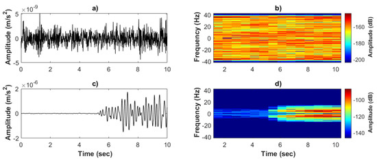
Figure 2.
The STFT results for a seismic signal and noise: (a) noise signal, (b) STFT spectrogram of noise, (c) P-wave part of seismic signal, and (d) STFT spectrogram of P-wave.
Therefore, Figure 2a was also sliced with 10 s of noise. Figure 2b,d correspond to the spectrogram images of the STFT results of the noise signal and P-wave signal, respectively. In this simulation, the STFT specification was set to have a sample rate of 85, a Kaiser window of length 256, and an overlap length of 220 samples. Figure 2b,d and Figure 2a,c clearly differ in the properties of the frequency component with the passage of time. Based on this difference, a deep learning model with the structure of GoogLeNet was designed as a binary classifier. The spectrogram images were image-processed as color images with a size of 224 × 224, which was the input data size of deep learning.
Figure 3 shows the accuracy and loss of the trained model. Training was performed using the spectrogram images obtained, such as those in Figure 2, as the training dataset. Although GoogLeNet is a structure with 10 outputs, we modified the model architecture as a binary classifier that distinguished the noise and P-wave labels for selecting the P-onset seismic signals. We collected 50,000 seismic and noise signals from the STEAD. We split this dataset into 75%, 5%, and 20% for training, validation, and testing, respectively. We trained this model at a learning rate of 1 for 360 epochs. According to the results in Figure 3a,b, the deep learning model was trained as a binary classifier with an accuracy of 98.5% and loss of 0.0353. The model converged with an accuracy of >90% at 250 epochs. One observatory detected seismic waves using three components. To estimate the P-onset, we predicted the P-wave using the trained model by dividing the three seismic waves into 200 windows, each with a window size of 10 s. The model output the probability of a P-onset using the STFT spectrogram images of the segmented windows as input data. Moreover, the first point with the highest probability was considered the P-onset.
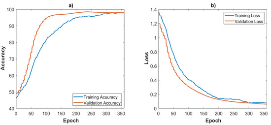
Figure 3.
The training and validation curves of the P-onset picking deep learning model: (a) model accuracy and (b) model loss.
Figure 4 shows an example of P-onset picking with seismic signals obtained from one of the stations that detected a seismic event on 2022-04-25-05:35:50-UTC. Figure 4a corresponds to the seismic waves analyzed with three components of an event, and Figure 4b is the STFT results for each seismic wave. We specified the P-onset by predicting the partitioned window using the trained deep learning model shown in Figure 3. According to Figure 4b, the red part of the 3D spectrogram image is the S-wave point according to the amplitude of the seismic waves. However, in our P-onset picking method, the point at which the prediction probability of the model first increased was designated as the P-onset. Therefore, we indicated the red lines at the point with the highest probability among the windows and predicted the P-onset before the S-wave point in Figure 4b. In this study, because the hypocenter was estimated using data from four stations, P-onset picking was required for the seismic waves detected at each station, as shown in Figure 4.
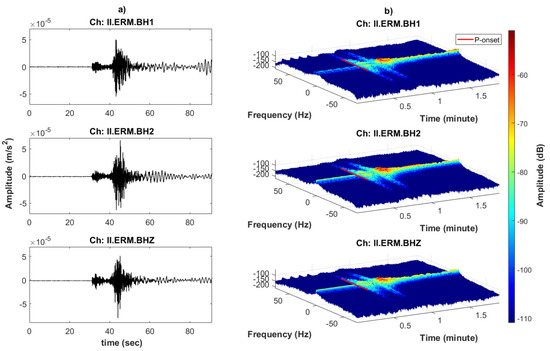
Figure 4.
P-onset picking example for an observatory: (a) seismic signals on three channels of an observatory and (b) P-onset picking prediction using the trained model.
Figure 5 shows the P-onset picking for the four observatories. Figure 5a–d correspond to the seismic waves from the four nearest stations for seismic events on 2022-04-25-05:35:50-UTC. The graphs in the first, second, and third rows of Figure 5a–c, and Figure 5d show the amplitudes of the seismic waves detected in the channel of the corresponding station. The figures in the fourth row shows the results of performing the same process as in Figure 4 at each observatory. In these figures, the trained deep learning model output the probability of the P-waves in the seismic waves of the corresponding observatory. The points with the highest probabilities are represented by red diamonds. Therefore, the estimated P-onsets redefined the distances between the hypocenter and the observatories.
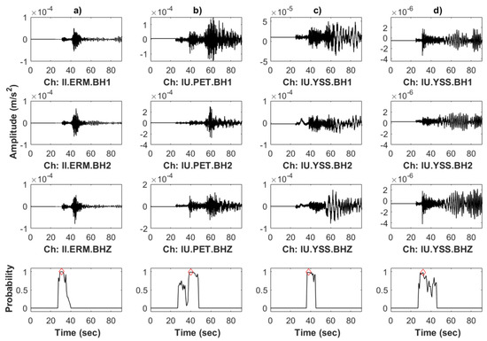
Figure 5.
P-onset picking for a seismic event detected by four observatories:(a–d) amplitudes and probabilities for seismic waves measured by each observatory.
Figure 6 shows the results of calibrating the distances between the hypocenter and observatories after P-onset picking for the actual seismic event on 2022-04-25-05:35:50-UTC. The black triangles represent each observatory, the blue star is the hypocenter, and the red solid lines are the actual distances between the hypocenter and observatories. In Figure 6a, the reported distances in the USGS and IRIS are expressed as a dashed black line. Figure 6b shows a scaled image expressing the certainty when the reported distances have a maximum certainty of 10. The certainty had a lower value as the distance from the reported distances increased. The degree of certainty is expressed as a color bar, where a higher certainty represents a warmer color. Typical values for P-wave propagation velocity in earthquakes are in the range of 5 to 8 km/s, according to bedrock and Earth models [30]. However, in this simulation, we specified the P-wave velocity to be 6.8 km/s. The redefined P-onsets derived the P-onset distances by considering the P-wave propagation speed. Figure 6c shows the calibrated distance after P-onset picking as a dashed blue line. Figure 6d shows a scaled image that expresses the certainty when the maximum P-onset distances have a certainty of 10. Compared with Figure 6b, the red area with high certainty was closer to the hypocenter through P-onset picking. Table 2 presents a numerical performance comparison for Figure 6. The distances shown in Table 2 correspond to the radii of the solid red circles, black dashed circles, and the blue dashed circles shown in Figure 6, respectively. Based on Table 2, the accurate distances were obtained by P-onset picking for all observatories. By calibrating the distance parameter used in the TDOA model to a value with high certainty, a more accurate hypocenter prediction was made.
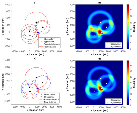
Figure 6.
Reported distance calibration and performance of P-onset picking: (a,b) reported seismic event and (c,d) performance of proposed method.
Table 2.
Numerical performance comparison for Figure 6.
Figure 7 presents the estimation of the hypocenter of the seismic event on 2022-04-25-05:35:50-UTC in 3D using localization methods. The black triangle is the observatory above the mean sea level, and the red star is the location of the hypocenter reported by the USGS and IRIS. The applied localization methods, the LS of the TDOA, the LS of the AOA, the LS of the TDOA/AOA, and the CLS of the TDOA/AOA, are represented by blue plusses, crosses, asterisks, and diamonds, respectively. The methods of applying the LS to the AOA and the CLS to the TDOA/AOA were confirmed to have good localization performance.
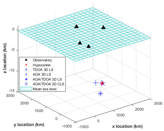
Figure 7.
Hypocenter estimation using the localization methods.
Figure 8 shows the results of expressing Figure 7 on the x–y plane to confirm the exact performance between the methods. The block area corresponds to a map that extends around the hypocenter. The estimation by the proposed TDOA/AOA CLS method (blue diamond) was closer to the red star, the hypocenter, than those by other methods. As shown in Figure 8, the proposed method was sufficiently precise to have an error of 45.3455 km from the actual hypocenter reported in the USGS and IRIS. In this simulation, the iterative process in Equation (20) was executed times, and the gradient descent rate was set to 6.5 . After the gradient descent process, the optimized solutions of were specified as −6.525 and −8.1029, respectively.
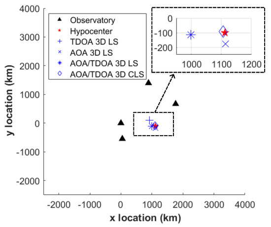
Figure 8.
Hypocenter estimation on the x–y plane using the localization methods.
Figure 9 shows the performance comparison between the other localization methods and the proposed method using the mean square error (MSE). The unit of the location was in kilometers, and the hypocenter was estimated using the proposed method for 10 seismic events. The first event on the x-axis in Figure 9 is the same as that introduced in Figure 4, Figure 5 and Figure 6. Other events were randomly selected from a dataset that occurred in the conterminous USA for one year, beginning on 2021-01-5-00:00:00 UTC. The deep-learning model trained on STEAD redefined the P-onset of all the seismic events. Seismic waves from four stations for each event were analyzed, and three localization algorithms were applied: the TDOA with LS, the TDOA/AOA with LS, and the TDOA/AOA with CLS indicated by a green plus, blue circle, and red square marked lines, respectively. The TDOA with the LS method had an average MSE of 275.5 km. The TDOA/AOA with the LS method had an average MSE of 152.7 km. The TDOA/AOA with the CLS method had a minimum average MSE of 70.2 km. These results also mean that the CLS estimation method had a lower root MSE, which was closer to the Cramer–Rao lower bound than the LS estimation method. Because the TDOA/AOA with the CLS method estimated the hypocenters closest to the real case, the proposed method showed the best estimation performance of hypocenter localization.
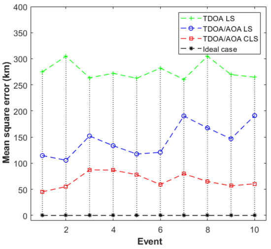
Figure 9.
Performance comparison for the proposed methods on the hypocenter localization.
5. Conclusions
This study proposed a hypocenter localization method using a hybrid TDOA/AOA and CLS with P-onset and DLT. We distinguished the noise and P-wave characteristics using STFT and constructed a dataset for deep learning through spectrogram image processing. With the excellent performance of GoogLeNet, the structure of the network was modified using a binary classifier to determine the noise and P-waves. After performing spectrogram image processing of seismic waves with three components at four stations using the STFT method, the probability of P-waves was derived using the pretrained deep learning model, and the distances between the observatories and hypocenter were corrected by determining the highest probability point of a P-wave as the P-onset. The proposed CLS efficiently improved the LS by minimizing the MSE. We only extended the dimension of the earthquake location for 3D positioning and overcame the limited horizontal performance of TDOA by combining it with AOA as a hybrid TDOA/AOA model. In this paper, the hybrid TDOA/AOA model for seismic localization was used for the first time. For accurate estimations using CLS, the hypocenter was optimized using a hybrid linear matrix equation. The Lagrange function was considered an objective function with two constraints, and the Lagrange multipliers were specified using an asymptotic gradient descent method. Simulations of various seismic events in a real environment verified the performance of the proposed method. According to the latest research trend, the performance of P-onset prediction with DLT can be improved by the emerging deep learning architecture. In addition, the proposed method is expected to apply for epicenter estimation in 2D.
Author Contributions
This research was accomplished by all the authors. H.A. and K.Y. conceived the idea, performed the analysis, and designed the simulation; H.K. and H.A. conducted the numerical simulations; H.A., A.C. and K.Y. co-wrote the manuscript. All authors have read and agreed to the published version of the manuscript.
Funding
This work was supported by the National Research Foundation of Korea (NRF) grant funded by the Korea government (MSIP) (NRF-2019R1A2C1002343) and the BK21 FOUR Project.
Institutional Review Board Statement
Not applicable.
Informed Consent Statement
Not applicable.
Data Availability Statement
The data presented in this study are available on Github from https://github.com/smousavi05/STEAD, accessed on 1 July 2022. The data are publicly available for AI research.
Conflicts of Interest
The authors declare no conflict of interest.
References
- Hsiao, N.; Wu, Y.; Shin, T.; Zhao, L.; Teng, T. Development of earthquake early warning system in Taiwan. Geophys. Res. Lett. 2009, 36, L00B022. [Google Scholar] [CrossRef]
- Nakamura, Y. On the urgent earthquake detection and alarm system (UrEDAS). In Proceedings of the 9th World Conference Earthquake Engring, Tokyo-Kyoto, Japan, 2–9 August 1988. [Google Scholar]
- Nepeina, K.; An, V. Travel timecurves and isochron maps from the Borovoye digital archive for the Nevada and Semipalatinsk nuclear test sites. Results Geophys. Sci. 2021, 6, 100014. [Google Scholar]
- Zuniga, N.; Priimenko, V. Automated travel-time picking using spectral recomposition. Braz. J. Geophys. 2021, 39, 375–392. [Google Scholar] [CrossRef]
- Saragiotis, C.; Hadjileontiadis, L.; Rekanos, I.; Panas, S. Automatic P phase picking using maximum Kurtosis and κ-statistics criteria. IEEE Trans. Geosci. Remote Sens. 2004, 1, 147–151. [Google Scholar] [CrossRef]
- Merino, J.; Herranz, J.; Parolai, S. Seismic P phase picking using a Kurtosis-based criterion in the stationary wavelet domain. IEEE Trans. Geosci. Remote Sens. 2008, 46, 3815–3826. [Google Scholar] [CrossRef]
- Kuperkoch, L.; Meier, T.; Lee, J.; Friederich, W. Automated determination of P-phase arrival times at regional and local distances using higher order statistics. Geophys. J. Int. 2010, 181, 1159–1170. [Google Scholar] [CrossRef]
- Guo, C.; Zhu, T.; Gao, Y.; Wu, S.; Sun, J. AEnet: Automatic picking of P-wave first arrivals using deep learning. IEEE Trans. Geosci. Remote Sens. 2021, 59, 5293–5303. [Google Scholar]
- Xu, H.; Zhao, Y.; Yang, T.; Wang, S.; Chang, Y.; Jia, P. An automatic P-wave onset time picking method for mining-induced microseismic data based on long short-term memory deep neural network. Geomat. Nat. Hazards Risk 2022, 13, 908–933. [Google Scholar] [CrossRef]
- Kaur, K.; Wadhwa, M.; Park, E. Detection and identification of seismic P-waves using artificial neural networks. In Proceedings of the 2013 International Joint Conference on Neural Networks (IJCNN), Dallas, TX, USA, 4–9 August 2013; pp. 1–6. [Google Scholar]
- Ross, Z.; Meier, M.; Hauksson, E. P wave arrival picking and first-motion polarity determination with deep learning. J. Geophys. Res. Solid Earth 2018, 123, 5120–5129. [Google Scholar] [CrossRef]
- Khan, I.; Kwon, Y. P-detector: Real-time P-wave detection in a seismic waveform recorded on a low-cost MEMS accelerometer using deep learning. IEEE Trans. Geosci. Remote Sens. 2022, 19, 1–5. [Google Scholar] [CrossRef]
- Lee, K.; Lee, H.; You, K. Optimised solution for hybrid TDOA/AOA-based geolocation using Nelder-Mead simplex method. IET Radar Sonar Navig. 2019, 13, 992–997. [Google Scholar] [CrossRef]
- Cong, L.; Zhuang, W. Hybrid TDOA/AOA mobile user location for wideband CDMA cellular systems. IEEE Trans. Wirel. Commun. 2002, 1, 439–447. [Google Scholar] [CrossRef]
- Zhao, Y.; Anagnostou, D.; Huang, J.; Sohraby, K. AOA based sensing and performance analysis in cognitive radio networks. In Proceedings of the 2014 IEEE National Wireless Research Collaboration Symposium, Idaho Falls, ID, USA, 15–16 May 2014; pp. 144–148. [Google Scholar]
- Yin, J.; Wan, Q.; Yang, S.; Ho, K. A simple and accurate TDOA-AOA localization method using two stations. IEEE Signal Process Lett. 2016, 23, 144–148. [Google Scholar] [CrossRef]
- Jia, T.; Wang, H.; Shen, X.; Jiang, Z.; He, K. Target localization based on structured total least squares with hybrid TDOA-AOA measurements. Signal Process. 2018, 143, 211–221. [Google Scholar] [CrossRef]
- Karasozen, E.; Karasozen, B. Earthquake location methods. GEM Int. J. Geomath. 2020, 11, 1–28. [Google Scholar] [CrossRef]
- Cheung, K.; So, H.; Ma, W.; Chan, Y. A constrained least squares approach to mobile positioning: Algorithms and optimality. EURASIP J. Adv. Signal Process. 2006, 2006, 1–23. [Google Scholar] [CrossRef]
- Zhang, B.; Wang, G.; Pang, Z.; Wang, B. Epicenter localization using forward-transmission laser interferometry. Opt. Express. 2022, 30, 24020–24030. [Google Scholar] [CrossRef]
- Lee, K.; Kwon, H.; You, K. Laser-interferometric broadband seismometer for epicenter location estimation. Sensors 2017, 17, 2423. [Google Scholar] [CrossRef] [PubMed]
- Gasparini, P.; Manfredi, G.; Zschau, J. Earthquake Early Warning Systems; Springer: Berlin, Germany, 2007. [Google Scholar]
- Zhu, W.; Sun, L.; Zhu, X. New estimation algorithm for epicenter location of low frequency seismograms. In Proceedings of the 2012 International Conference on Systems and Informatics (ICSAI2012), Yantai, China, 19–20 May 2012; pp. 1706–1710. [Google Scholar]
- Oh, J.; Lee, K.; You, K. Hybrid TDOA and AOA Localization Using Constrained Least Squares. IEICE Trans. Fundam. Electron. Commun. Comput. Sci. 2015, E98-A, 2713–2718. [Google Scholar] [CrossRef]
- Szegedy, C.; Liu, W.; Jia, Y.; Sermanet, P.; Reed, S.; Anguelov, D.; Erhan, D.; Vanhoucke, V.; Rabinovich, A. Going deeper with convolutions. In Proceedings of the IEEE Conference on Computer Vision and Pattern Recognition, Boston, MA, USA, 7–12 June 2015. [Google Scholar]
- Du, H.; Lee, J. Simulation of multi-platform geolocation using a hybrid TDOA/AOA method. In Proceedings of the Technical Memorandum of Defence Research and Development Canada-Ottawa, TM 2004–256, Ottawa, ON, Canada, 1 December 2004. [Google Scholar]
- Huang, Y.; Benesty, J.; Elko, G.W.; Mersereati, R.M. Real-time passive source localization: A practical linear-correction least-squares approach. IEEE Trans. Speech Audio Process. 2001, 9, 943–956. [Google Scholar] [CrossRef]
- United States Geological Survey. Available online: https://earthquake.usgs.gov (accessed on 1 July 2022).
- Mousavi, S.; Sheng, Y.; Zhu, W.; Beroza, G. Stanford earthquake dataset (STEAD): A global data set of seismic signals for AI. IEEE Access 2019, 7, 179464–179476. [Google Scholar] [CrossRef]
- Selley, R.; Cocks, R.; Plimer, I. Encyclopedia of Geology; Academic Press: London, UK, 2005. [Google Scholar]


Publisher’s Note: MDPI stays neutral with regard to jurisdictional claims in published maps and institutional affiliations. |
© 2022 by the authors. Licensee MDPI, Basel, Switzerland. This article is an open access article distributed under the terms and conditions of the Creative Commons Attribution (CC BY) license (https://creativecommons.org/licenses/by/4.0/).