Article

Numerical Simulation of Multifracture Growth under Extremely Limited Entry Fracturing of Horizontal Well

1
Yan’an Energy Service Co., Ltd., Yanan 716099, China
2
Yan’an Unconventional Natural Gas Research Institute, Yanan 716099, China
3
College of Petroleum Engineering, China University of Petroleum (East China), Qingdao 266580, China
4
Research Institute of Petroleum Exploration & Development, Beijing 100083, China
5
College of Petroleum Engineering, Southwest Petroleum University, Chengdu 610500, China
*
Author to whom correspondence should be addressed.
Processes 2022, 10(12), 2508; https://doi.org/10.3390/pr10122508
Submission received: 23 October 2022 / Revised: 15 November 2022 / Accepted: 21 November 2022 / Published: 25 November 2022

Abstract

:
The multifracture competitive growth from a horizontal well is an essential issue in multi-cluster fracturing design. In recent years, extremely limited entry (ELE) fracturing has been implemented to promote uniform multifracture growth. However, the mechanism of multifracture growth and ELE design remain unclear. Based on the planar three-dimensional multifracture propagation model, a multi-cluster horizontal well fracturing model that considers ELE design has been developed. The model considers flow in the wellbore and fluid filtration loss in the fracture. The simulator enables the simulation and analysis of non-uniform in situ stress, filtration loss, and fracture properties. Using this program, we simulated the propagation process of multiple clusters of fractures in ELE fracturing of horizontal wells. The results show the following: The perforation friction in the ELE fracturing can counteract the difference in fluid allocation caused by stress interference, allowing all clusters of perforations to have even fluid allocation but to differ significantly in fracture geometry. The in situ stress profile and 3D fracture stress interference determine the fracture geometry, and the fracture of the middle cluster could cross through the layer with relatively higher in situ stress, resulting in a decrease in effective fracture area in the pay zone. Furthermore, an increase in perforation diameter causes the flow-limiting effect of the perforations to decrease. The fluid volumes entering different clusters of perforations become less uniform. The difference in fracture toughness within a perforated stage has a minor influence on the fluid allocation between different clusters, while the in situ stress distribution within a perforated stage has a significant impact on the fluid allocation between different perforation clusters in the stage. Fractures preferentially propagate at the perforation points with lower in situ stress and stress interference. This study can be helpful to understand multifracture competitive growth and the optimization of ELE fracturing design.

1. Introduction

Multi-cluster fracturing technology for petroleum and geothermal energies is the primary technology of reservoir stimulation under the current low oil prices [1,2]. Temperature and acoustic monitoring with optical fiber and perforation imaging after the multi-cluster fracturing of horizontal wells have revealed non-uniform fluid allocation between different clusters of fractures [3,4,5]. Non-uniform fluid allocation between different perforation clusters may lead to a fast extension of some fractures and a premature stop in others, and, thus, a decrease in stimulated reservoir volume, making fracturing design challenging [6].
The multifracture propagation mechanism is currently mainly analyzed theoretically by numerical simulation. The main simulation methods include the finite element, extended finite element, discrete element, and boundary element method [7]. The finite element, extended finite element, and discrete element methods are full-field discretization techniques with high storage and computational costs. In contrast, the boundary element method only requires discretization at the fractures and, thus, is less computationally intensive and is better for engineering applications, particularly for fracture simulation [8]. It has been found that reservoir heterogeneity and stress interference between multiple fractures are the primary factors that affect the uneven propagation of multiple fractures [9,10,11,12]. To promote the simultaneous propagation of multiple fractures, Shell proposed an extremely limited entry (ELE) operation in 2018 [12]. In this process, the perforation friction is significantly increased and the number of perforations is limited to 2–3/clusters to achieve uniform fracture initiation and fluid allocation between different fracture clusters. To date, the effectiveness of limited entry fracturing is mainly based on simulation results from two-dimensional (2D) and pseudo-three-dimensional (P3D) fracture propagation models, and the growth pattern of multi-cluster fractures in ELE fracturing in three-dimensional fracture morphology has scarcely been studied [13,14]. Meanwhile, the ELE fracturing process was tested in China in the fracturing operations of Shengli shale oil and Fuling shale gas reservoirs [14]. Analysis methods for this fracturing process must be urgently developed to demonstrate their effectiveness.
The hydraulic fracture simulation model is an effective way to optimize fracturing design [15]. It contains 2D, P3D, planar 3D (PL3D), and fully 3D models. The 2D and P3D models are typically used in the industry due to their high efficiency, while the PL3D and fully 3D models have increased accuracy but are less efficient. A comprehensive review of the four kinds of models can be found in [16] and [17]. Recently, drilling cores and distributed acoustic sensing from adjacent wells show that fractures are mostly planar in the reservoir scale [18,19,20,21]. These results demonstrate that using PL3D is the best choice for optimizing fracturing design due to its accuracy and efficiency [22].
Therefore, a planar 3D multifracture propagation model was proposed in this work based on our previous work [22,23,24,25], the extension of multiple fractures in extremely limited entry fracturing was simulated numerically using parameters of a shale oil well to demonstrate the effectiveness of this fracturing method in the hope of providing a reference basis for fracturing design.
The paper is organized as follows. The mathematical model of the planar 3D multifracture is given in Section 2. Section 3 presents the numerical scheme for the mathematical model. A case study from the Shengli shale oil formation is then conducted and analyzed in Section 3. A parametric sensitivity is conducted in Section 4. Finally, conclusions are drawn in Section 5.

2. Mathematical Model

Fracture models are simplifications of actual fractures, so recognizing real fracture patterns is the first step in fracture modeling. Many observations and interpretations have been performed to find patterns of fractures generated in fracturing. The most reliable method to find fracture patterns is the observation of drilled cores containing hydraulic fractures. Many planar fractures were found in cores taken from shale gas wells after fracturing in the United States [20], complex fractures were only seen in local parts, so it is reasonable to simplify the fractures as planar fractures on a macroscopic level [21]. Meanwhile, unconventional oil and gas reservoirs in China generally have large horizontal stress differences [13], so it is difficult for them to be deflected theoretically, which further confirms that simplifying fractures into planar fractures is reasonable. Therefore, in this work, the fractures were assumed to extend along a fixed plane, i.e., the assumption of a planar three-dimensional fracture model was adopted.

2.1. Governing Equations

Hydraulic fracturing is a fracture-extension process driven by high-pressure viscous fluid and consists of four main physical processes: rock deformation, fluid flow in the fracture, fluid filtration loss to the formation, and fracture propagation at the fracture tip [26]. For multi-cluster fracturing of a horizontal well, it also includes fluid distribution through the wellbore. The geometric model is shown in Figure 1.

2.1.1. Elasticity

A three-dimensional displacement discontinuity method (DDM) was used to calculate the rock deformation. The advantage of DDM is that it reduces the problem by one dimension, so the computation burden is less than FEM or extended FEM. However, the disadvantage of the DDM used in our model is based on 3D Green’s function of dislocation dipoles in a linear elastic media with uniform elastic properties, so the heterogeneous elastic properties cannot be considered. In contrast, such properties can be easily handled by FEM or extended FEM. In our model, we use the boundary element method to solve solid elasticity, as it is suitable for the fracture problems in an infinite domain.
The amount of shear displacement discontinuity for planar fracture extension is zero. Therefore, the relationship between pressure in a fracture and the fracture width can be described by Equation (1) [27]:
p f σ h = A ( t ) C ( x x , y y , z z ) w ( x , y , z ) d A
where pf is the fluid pressure, MPa; σh is the minimum horizontal principle stress, MPa; C is the Green’s function; t is the time, s; A(t) is the area of opened fracture at moment t, m2; w is the fracture width, m; (x′, y′, z′) are the coordinates of the source point; and (x, y, z) are the coordinates of the field point.
The specific form of Green’s function C is [27]
C = E 8 π ( 1 v 2 ) 1 [ ( x x ) 2 + ( y y ) 2 + ( z z ) 2 ] 1.5
where E is Young’s modulus, MPa, and v is Poisson’s ratio, dimensionless.

2.1.2. Fluid Flow in a Fracture

Assuming that the fluid flow inside the fracture conforms to Poiseuille flow [28], the constitutive equation of fluid flow inside the fracture is
q = w 3 12 μ p f
where q is the volume flow rate, m2/s, and μ is the fluid viscosity, Pa·s.
The component form of Equation (2) is
{ q x = w 3 12 μ p f x q y = w 3 12 μ p f y
where qx and qy are the volume flow rates in the x direction and the y direction, respectively.
The continuity equation of fluid flow in the fracture is
w t + q + 2 C l t t 0 = δ ( x x in , k , y y in , k , z z in , k ) Q k ,   k = 1 , 2 , , n f
where Qk is the flow rate at the inlet of fracture k, m3/s; Cl is the filtration loss coefficient, m/min0.5; t0 is the moment when filtration loss starts, min; nf is the number of fractures; and (xin,k, yin,k, zin,k) are the coordinates of the inlet of fracture k.
Substituting Equation (3) into Equation (5), the following transport equation is obtained:
w t = ( w 3 12 μ p f ) + 2 C l t t 0 + δ ( x x in , k , y y in , k , z z in , k ) Q k ,   k = 1 , 2 , , n f

2.1.3. Wellbore Conditions

In multi-cluster fracturing, the injected fracturing fluid passes through the wellbore and perforations into different clusters of fractures. The amount of fluid entering each cluster is controlled by the “wellbore–perforation–fracture” system. The pressure at the inlet of each fracture cluster satisfies [29]
p w = p p , k + p t , k + p in , k ,   k = 1 , 2 , , n f
where pt,k is the wellbore flow friction of fracture k, MPa; pp,k is the friction of perforation corresponding to fracture k, MPa; and pin,k is the pressure at the inlet of fracture k, MPa.
The friction of perforation is calculated by [30]
p p , k = 0.807 ρ Q k 2 n k 2 d k 4 K k 2
The flow friction in the wellbore is calculated by Churchill’s entire flow equation [31].
At the same time, the flow rates of all clusters satisfy the mass conservation law, i.e.,
Q T = I = 1 n f Q in , k

2.2. Initial Boundary Condition

The flow at inlet of each fracture satisfies
Q | in = w 3 12 μ p n = Q in , k
The flow at the fracture boundary is zero, i.e.,
Q | A = w 3 12 μ p n = 0
When the stress intensity factor at the fracture tip reaches the rock fracture toughness, the fracture starts to grow.
K tip = K Ic
where KIc is the rock type I fracture toughness, MPa·m0.5.
The calculation equation of the tip stress intensity factor is [32]
K tip = 0.806 E π w tip 4 ( 1 v 2 ) d
where wtip is the width of the fracture tip cell, m, and d is the length of the tip cell, m.

3. Numerical Scheme

A fixed grid (rectangular cell-structured grid) was used to calculate the fracture-extension process. The cell was labeled as (i,j,k), and the corresponding position was (xi,yj,zk). There were four types of cells: channel cells, tip cells, cells to be activated, and inactive cells (Figure 2). The cell type of the grid system was updated each time by determining whether the tip cell met the propagation condition. The cell’s center point was the unknown quantity (width and pressure) solution point, and the cell boundary was the position of the flow rate.
All open cells and tip cells were labeled sequentially as I, and the number of cells at the current moment was Ne, I = 1, 2, ..., Ne. Equation (1) was discretized by the constant displacement discontinuity method.
p I = J = 1 N e C I J w J + σ h
where Ne is the number of cells, and the capital I and J cell number labels were used to distinguish from the overall cell serial number (i,j,k). CIJ was derived from Equation (2).
The matrix form of Equation (14) is
p = C w + σ h
The discrete form of the flow Equation (6) was established by the finite volume method:
Δ w i , j , k = Δ t 12 μ d x [ ( w i + 1 2 , j , k 3 p i + 1 , j , k p i , j , k d x w i 1 2 , j , k 3 p i , j , k p i 1 , j , k d x ) ] + Δ t 12 μ d y [ ( w i , j + 1 2 , k 3 p i , j + 1 , k p i , j , k d y w i , j 1 2 , k 3 p i , j , k p i , j 1 , k d y ) ] 4 C l t t 0 + Δ t Q k
To calculate the wellbore flow distribution according to the wellbore conditions, we use
F ( Q 1 , Q 2 , , Q n f , p w ) = 0
The specific components of Equation (17) are
{ F 1 ( Q 1 , Q 2 , , Q n f , p w ) = p w 0.807 ρ Q 1 2 n 1 2 d 1 4 K 1 2 p t , 1 p i n , 1 ( Q 1 , Q 2 , , Q n f , p w ) F k ( Q 1 , Q 2 , , Q n f , p w ) = p w 0.807 ρ Q k 2 n k 2 d k 4 K k 2 p t , 1 p i n , k ( Q 1 , Q 2 , , Q n f , p w ) F n f ( Q 1 , Q 2 , , Q N , p w ) = p w 0.807 ρ Q N 2 n n f 2 d n f 4 K n f 2 p t , 1 p i n , n f ( Q 1 , Q 2 , , Q n f , p w ) F n f + 1 ( Q 1 , Q 2 , , Q N , p w ) = Q T k = 1 n f Q k
The Newton–Raphson method was used to solve Equation (17), and the solution was iterated by coupling Equations (15) and (16) to calculate the flow rate of each cluster. The coupling equations were solved by the second-order Rough–Kutta–Legendre method. It uses strategically devised explicit RK stages to stabilize the solution, with larger time-steps than that of the explicit Euler finite difference scheme. The timestep was determined adaptively based on the fracture propagation velocity. The accuracy of the model was fully validated by penny fracture analytical solutions, hydraulic fracturing physical modeling experiments, and published literature results; see the details in References [22,23,24,25]. The model is solved programmatically using MATLAB (2020a), and the calculations are fully vectorized with high computational efficiency [33,34].

4. Results and Analysis of a Field Well

Parameters of a shale oil well X in Shengli Oilfield were taken for fracture extension calculation and analysis. The well was treated by ELE fracturing with slick water as the fracturing fluid. Each fracturing stage had six clusters of fractures at an average fracture spacing of 15 m. The locations of the horizontal well and fracture clusters are shown in Figure 3. The horizontal in situ stress difference at the wellbore is 12 MPa, so the fractures are mainly planar fractures. The perforation parameters were three perforations with 12 mm diameters in one cluster, discharge coefficients of 0.8, a fracturing fluid density of 1030 kg/m3, and an injection rate of 10 m3/min. Microfractures and natural fractures in the formation can increase the fluid filtration loss, so a larger filtration loss coefficient, 2 × 10⁻⁴ m/min0.5, was taken.

4.1. Base Case

Figure 4 shows patterns of the fractures of the base case. To clearly demonstrate the patterns of the fractures, three-dimensional (Figure 4a) and planar (Figure 4b) graphs of all the fractures, and planar graphs (Figure 4c) of each fracture were drawn separately. The plane with y = 0 in Figure 3 was the perforation point (injection point). Since multiple fractures extend along the paths with the lowest energy dissipation of the system, the fractures have large differences in length and height. For example, the HF2, HF4, and HF5 fractures have larger heights, and nearly half of the fracture areas in the low-stress layer lie above the perforation section.
The variation coefficient of fluid allocation is defined as
V d = V max V min V ¯ × 100 %
where V max   , V m i n ,   and   V ¯ are the cluster with the maximum fluid volume allocation, the cluster with minimum fluid volume allocation, and the average fluid volume allocation of the clusters in m3, respectively. Compared with measuring the variation coefficient of fluid allocation with a standard deviation, this parameter is more intuitive.
Figure 5 shows the flow and fluid volume allocation of each cluster. The heel-side fracture had the maximum fluid volume, while the middle fracture had the lowest fluid volume. This observation results from the stress interference among multiple fractures. The middle fracture takes more interaction stresses induced by other fractures. According to Equation (19), the variation coefficient of fluid allocation was calculated at 9.1%.
Figure 6 shows the inlet width and area of each cluster of fractures. The results show that the fracture width generated by ELE fracturing ranged from 1.8 to 2.3 mm, with a range of 0.5 mm. However, the fractures had small differences in total area, as shown in Figure 6b.
Figure 7 shows the friction of each cluster perforation and bottom-hole pressure. The results show that the different clusters of perforations (three perforations with 12 mm diameters in one cluster) had friction values of 5–6 MPa at an injection rate of 10 m3/min. This friction could counteract the differences in fluid resistance caused by stress interference between the fractures. Therefore, the fluid volumes entering the fractures were relatively uniform. Despite the uniform fluid allocation, the different clusters of fractures vary widely in shape because fracture extension morphology is controlled by both in situ stress and stress interference between fractures [29]. Multiple fractures take the propagation paths with the lowest energy consumption (the embodiment of the principle of least action).

4.2. Effect of Perforation Diameter

In this section, the influence of perforation diameter was analyzed. Due to erosion of the fluid and proppant, perforations are subject to abrasion during the fracturing process and increase in diameter to varying degrees. Perforation abrasion models are mostly developed from the results of surface experiments, which are quite different from the monitoring of downhole abrasion. In this section, the effect of perforation diameter was analyzed by changing the perforation diameter from 10–= to 16 mm.
Figure 8 shows the extension patterns of six clusters of fractures at different perforation diameters. Figure 9 shows the patterns of fractures (HF1) at the heel at different perforation diameters.
Figure 10 shows the fluid allocations at different perforation diameters. Figure 11 shows the relationship between fluid allocation and the perforation diameter variation coefficient. Figure 10 and Figure 11 show that as the perforation diameter increases, the variance coefficient of fluid allocation increases. When the perforation diameter increases from 10 mm to 16 mm, the variation coefficient of fluid allocation increases from 5% to 30%. Perforations may increase by 50–120% in diameter after fracturing according to field monitoring, so even in extremely limited entry fracturing, fluid volumes entering different clusters of fractures may still be uneven.

4.3. Fracture Toughness Heterogeneity of Perforated Sections

Four cases were simulated to determine the effect of fracture toughness heterogeneity in a perforated stage. The heterogeneous fracture toughness was set to increase linearly at 0.25 MPa·m0.5, 0.5 MPa·m0.5, 0.75 MPa·m0.5, and 1 MPa·m0.5 per cluster from HF1 to HF6, respectively.
Figure 12 shows the patterns of fractures and fluid allocations in each of the four cases. Figure 13 shows the relationship between the heterogeneous fracture toughness and the variation coefficient of fluid allocation. Figure 13 shows that the variation coefficient of fluid allocation decreases with the increase in heterogeneous fracture toughness. However, the variation amplitude is small, so the influence of heterogeneous fracture toughness between clusters on fluid allocation between different clusters is also small. This is because the bottom-hole pressure is high in ELE fracturing. The high bottom-hole pressure is sufficient to counteract the fracture pressure differences caused by the heterogeneous fracture toughness of different clusters.

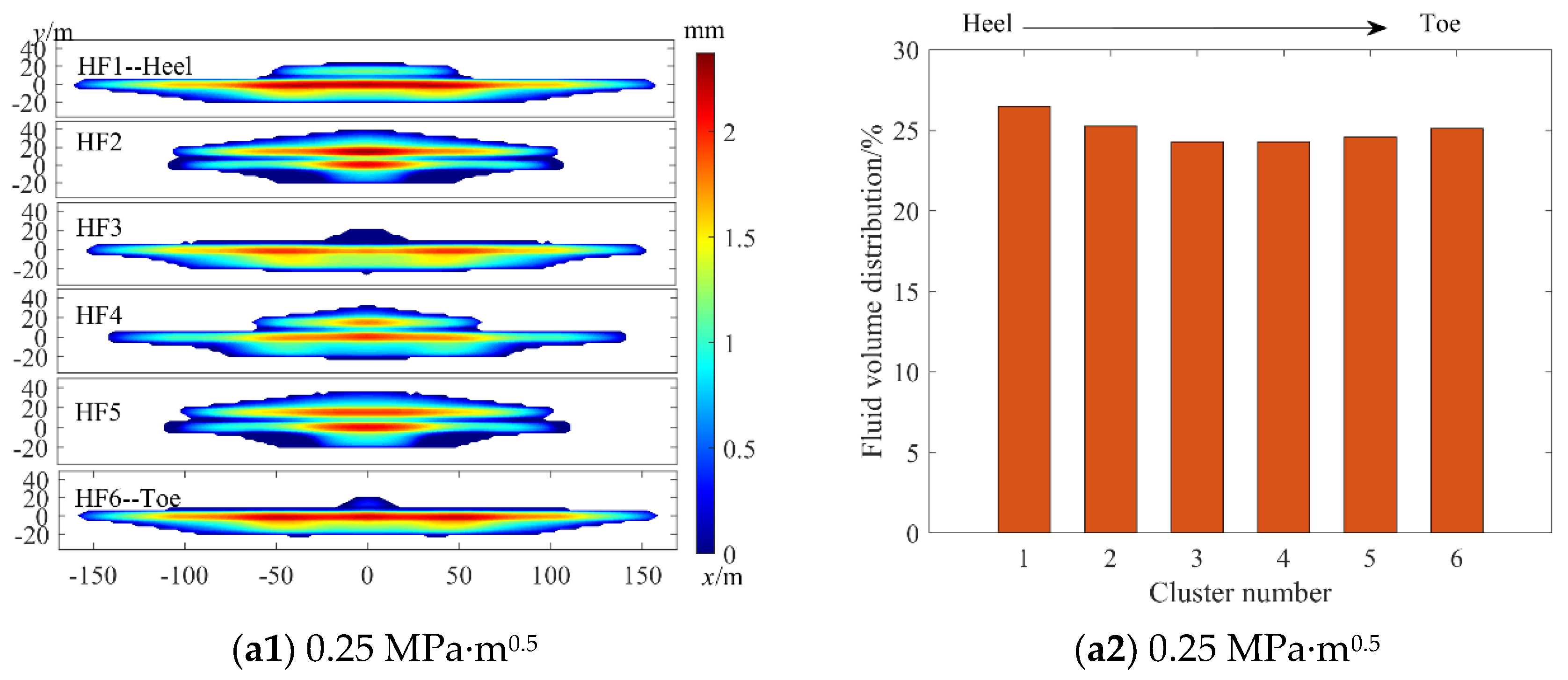
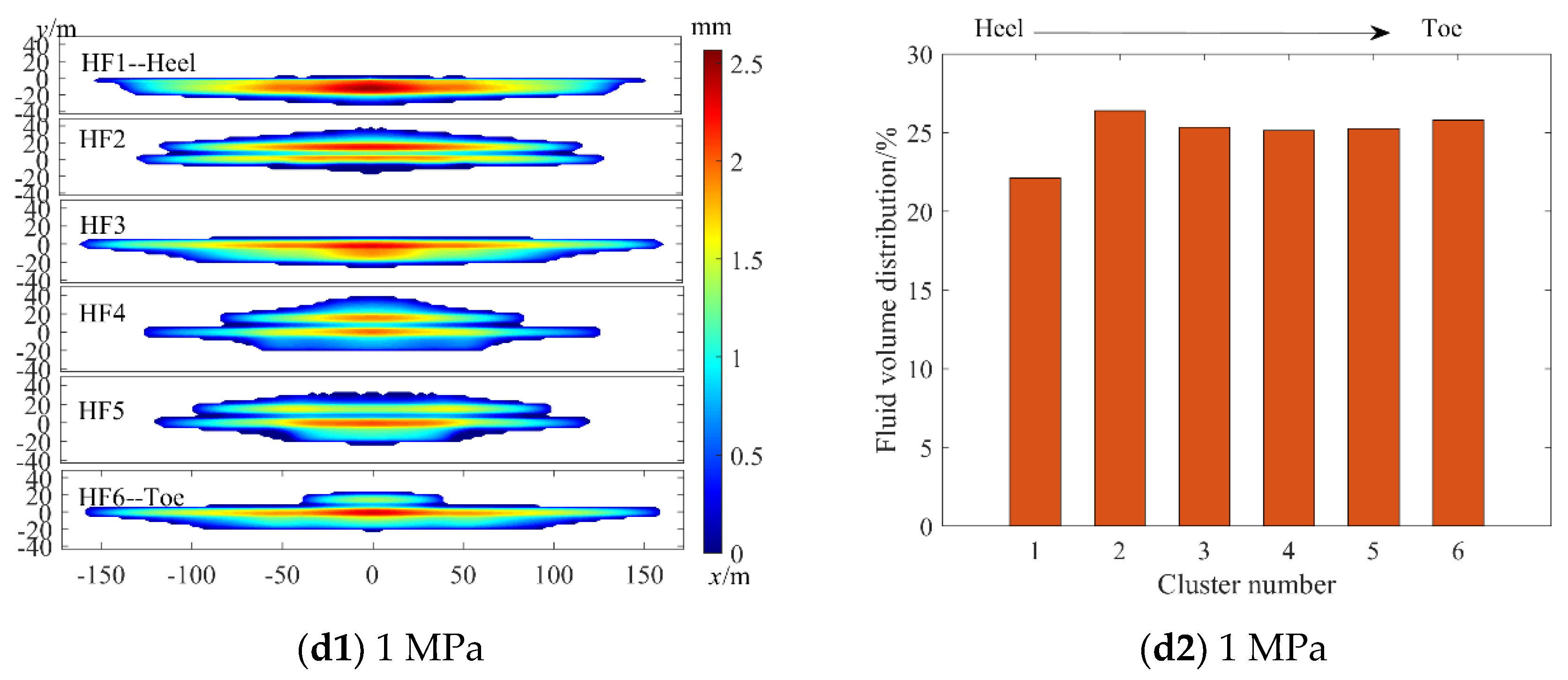
4.4. Heterogeneous In Situ Stress of the Perforated Section

Four different cases of heterogeneous in situ stress were simulated, in which the perforated section containing HF1 to HF6 fractures with heterogeneous fracture toughness was set to linearly increase the minimum horizontal principal stress. The stresses were set to 0.25 MPa, 0.5 MPa, 0.75 MPa, and 1 MPa per cluster from HF1 to HF6, respectively. Figure 14 shows the fracture geometry and fluid volume distribution among multiple fractures for different in-stage in-situ stress distributions. It can be observed that the multifracture geometry differs minorly among different in-situ stress distributions; whereas with the increase of in-situ stress in a perforation cluster, the fluid volume decreases significantly. Figure 15 shows that, for the well in this study, the variation coefficient of fluid allocation does not vary monotonically with the stress differences between clusters. When the stress difference between two clusters is less than 0.5 MPa, the variation coefficient of fluid allocation decreases with an increase in stress difference. In contrast, when the stress difference between two clusters is greater than 0.5 MPa, the variation coefficient of fluid allocation increases with an increase in stress difference between two clusters. This variation pattern is caused by an extremely limited entry fracturing operation mode and the profile of interlayer stress. When the stress difference between two clusters is less than 0.5 MPa, the friction of extremely limited entry flow can counteract the in situ stress difference between clusters, allowing the fluid allocation between clusters to be relatively uniform. In contrast, when the stress difference between clusters is higher, at 0.5 MPa for example, the fractures at the toe end section with higher in situ stress tend to propagate to the layer above the perforated section with lower in situ stress. When the fractures at the toe-end enter the layer with lower in situ stress, the stress interference between the fracture clusters reduces due to uneven widths of fractures longitudinally. This further reduces the difference in fluid allocation between the clusters. When the stress difference between the clusters is higher than 0.5 MPa, the difference in fluid allocation between the clusters is dominated by the stress difference between the clusters. Thus, the variation coefficient of fluid allocation increased with the increase in stress difference between the clusters.

4.5. Therotiecal Analysis of Fluid Allocation among Multiple Fractures

The parameter analysis above reveals that the fluid distribution among multiple fractures for ELE fracturing is primarily uniform due to high perforation friction. In this section, we provide a theoretical method to analyze this observation. The flux distribution of fluid flow is similar to current flow in an electrical circuit network, as shown in Figure 16. Without considering the wellbore friction, each fracture has the same pressure drop. The flow rate in each fracture is thus dependent on the flow resistance in the deformable fracture and perforations. The total pressure drop is calculated as
Δ p = p w p 0 = f p , k Q k 2 + f f , k Q k
where Δ p is the pressure drop, MPa; pw is the wellbore pressure, MPa; p0 is the pore pressure, MPa; f p , k is the coefficient of perforation friction for the kth fracture; and f h f , k is the coefficient of fluid flow friction in the kth fracture.
The resistance of flow in a hydraulic fracture should be solved by the solid-fluid coupling equations, where the stress shadowing effect and spatial variation of in situ stresses play an important role. The resistance of flow through perforations is calculated by Equation (8).
For the coupled system, the perforation friction, spatial variation of in situ stress, and flow friction in each fracture (dependent on stress shadowing effect, etc.) control the flow distribution among each fracture. For ELE fracturing, the perforation friction is much higher than the interaction stresses among multiple fractures. Thus, Equation (20) shows that, when all the fractures have the same perforation parameters, fluid allocation is relatively uniform.

5. Conclusions

In this work, a planar three-dimensional multifracture extension model coupling wellbore flow was developed, and the fracture extension dynamics in extremely limited entry fracturing were analyzed with this model. Through the study, the following conclusions have been reached:
(1)
The perforation friction in extremely limited entry fracturing of up to 5–6 MPa can counteract the difference in fluid allocation between fracture clusters caused by stress interference, resulting in an even fluid allocation between different clusters of perforations.
(2)
The path of hydraulic fracture reflects the principle of least action. In other words, fractures automatically grow along paths with the least resistance. Although fluid allocation between different fracture clusters in extremely limited entry fracturing is quite even, fractures of different clusters vary widely in geometry. The in situ stress profile and 3D fracture stress interference are the major factors affecting the patterns of fractures; fractures of the middle clusters could cross layers, causing the effective fracture area within the pay zone to decrease.
(3)
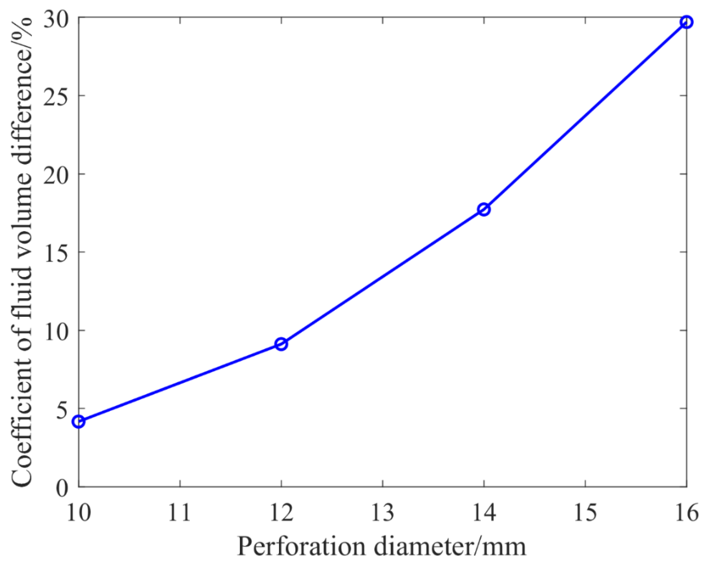
With an increase in perforation diameter, the flow limiting effect decreases, and the fluid allocation between clusters of fractures becomes less uniform.
(4)
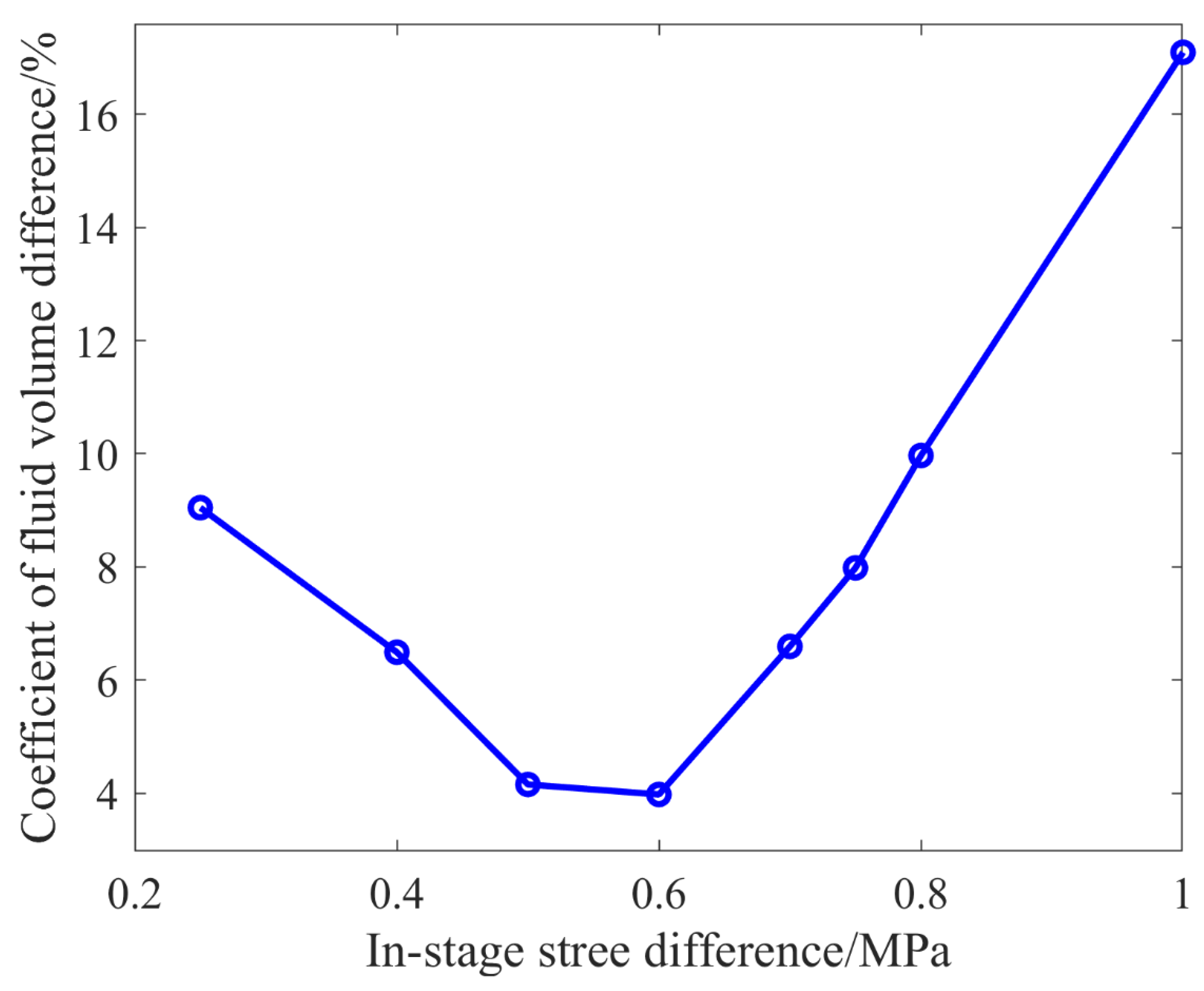
The fracture toughness difference in a perforated section has little effect on the fluid allocation between different clusters of fractures in the section. In contrast, the stress distribution in a perforated section significantly affects the fluid allocation between the clusters of perforations. Fractures preferentially extend at perforation clusters with lower in situ stress and stress interference.
(5)
The reasonable perforation erosion model should be investigated to further analyze the effectiveness of ELE fracturing in future studies.

Author Contributions

Writing, review, and editing, T.W., M.C. and D.W.; Methodology, M.C. and Y.X.; Software, Z.Y.; Results analysis, Z.L.; Visualization, Z.M. and H.J. All authors have read and agreed to the published version of the manuscript.

Funding

The research was supported by the Shandong Provincial Natural Science Foundation (ZR2021QE015), the National Natural Science Foundation of China (51874338), and the major project of CNPC (2021DJ4506, 2021DJ4502).

Data Availability Statement

This is a theoretical work for which no data need to be available.

Conflicts of Interest

The authors declare no conflict of interest.

References

  1. King, G. Thirty Years of Gas Shale Fracturing: What Have We Learned? In Proceedings of the Presented at the SPE Annual Technical Conference and Exhibition, Florence, Italy, 19–22 September 2010. SPE-133456-MS. [Google Scholar]
  2. Guo, T.; Zhang, Y.; Zhang, W.; Niu, B.; He, J.; Chen, M.; Yu, Y.; Xiao, B.; Xu, R. Numerical simulation of geothermal energy productivity considering the evolution of permeability in various fractures. Appl. Therm. Eng. 2022, 201, 117756. [Google Scholar] [CrossRef]
  3. Ramurthy, M.; Richardson, J.; Brown, M.; Sahdev, N.; Wiener, J.; Garcia, M. Fiber-Optics Results from an Intra-Stage Diversion Design Completions Study in the Niobrara Formation of DJ Basin. In Proceedings of the Presented at the SPE Hydraulic Fracturing Technology Conference, The Woodlands, TX, USA, 9–11 February 2016. SPE-179106-MS. [Google Scholar]
  4. Roberts, G.; Lilly, T.B.; Tymons, T.R. Improved Well Stimulation Through the Application of Downhole Video Analytics. In Proceedings of the Presented at the SPE Hydraulic Fracturing Technology Conference and Exhibition, The Woodland, TX, USA, 23–25 January 2018. SPE-189851-MS. [Google Scholar]
  5. Cramer, D.; Friehauf, K.; Roberts, G.; Whittaker, J. Integrating DAS, treatment pressure analysis and video-based perforation imaging to evaluate limited entry treatment effectiveness. In Proceedings of the Paper Presented at the SPE Hydraulic Fracturing Technology Conference and Exhibition, The Woodlands, TX, USA, 5–7 February 2019. SPE 194334. [Google Scholar]
  6. Evans, S.; Holley, E.; Dawson, K.; Garrison, N.; Montes, M.; Preston, G.; Hudson, S. Eagle Ford Case History: Evaluation of Diversion Techniques to Increase Stimulation Effectiveness. In Proceedings of the Presented at the SPE/AAPG/SEG Unconventional Resources Technology Conference, San Antonio, TX, USA, 1–3 August 2016. URTeC 2459883. [Google Scholar]
  7. Zhang, S.C.; Chen, M.; Ma, X.; Zou, Y.S.; Guo, T.K. Research progress and development direction of hydraulic fracturing design model. Xinjiang Oil Gas 2021, 17, 67–73. [Google Scholar]
  8. Jin, Y.; Cheng, W.; Chen, M. Advances in numerical simulation techniques for fracturing shale gas reservoirs. Mech. Prac. 2016, 38, 1–9. [Google Scholar]
  9. Bunger, A.; Cardella, D.J. Spatial distribution of production in a Marcellus shale well: Evidence for hydraulic fracture stress interaction. J. Petrol. Sci. Eng. 2013, 133, 162–166. [Google Scholar] [CrossRef]
  10. Lecampion, B.; Desroches, J.; Weng, X.; Burghardt, J.; Brown, J.E. Can we engineer better multistage horizontal completions? evidence of the importance of near-wellbore fracture geometry from theory, lab and field experiments. In Proceedings of the Presented at the SPE Hydraulic Fracturing Technology Conference, The Woodlands, TX, USA, 3–5 February 2015. [Google Scholar]
  11. Manchanda, R.; Bryant, E.; Bhardwaj, P.; Cardiff, P.; Sharma, M.M. Strategies for effective stimulation of multiple perforation clusters in horizontal wells. SPE J. 2018, 33, 539–556. [Google Scholar] [CrossRef]
  12. Somanchi, K.; Brewer, J.; Reynolds, A. Extreme limited-entry design improves distribution efficiency in plug-and-perforate completions: Insights from fiber-optic diagnostics. SPE J. 2018, 33, 298–306. [Google Scholar] [CrossRef]
  13. Zhao, J.Z.; Chen, X.Y.; Li, Y.M.; Fu, B.; Xu, W.J. Simulation analysis and shot hole optimization of segmented multi-cluster fracturing in horizontal wells. Pet. Explor. Dev. 2017, 44, 117–124. [Google Scholar] [CrossRef]
  14. Hou, B.; Chang, Z.; Wu, A.A.; Derek, E. Simulation of competitive propagation of multifractures on shale oil reservoir multi-clustered fracturing in Jimsar sag. Acta Petrol. Sin. 2022, 43, 75–90. [Google Scholar]
  15. Linkov, A.M. Modern theory of hydraulic fracture modeling with using explicit and implicit schemes. Comput. Eng. Financ. Sci. 2019. Available online: https://arxiv.org/abs/1905.06811 (accessed on 18 May 2019).
  16. Adachi, J.; Siebrits, E.; Peirce, A.; Desroches, J. Computer simulation of hydraulic fractures. Int. J. Rock Mech. Min. 2007, 44, 739–757. [Google Scholar] [CrossRef]
  17. Lecampion, B.; Bunger, A.; Zhang, X. Numerical methods for hydraulic fracture propagation: A review of recent trends. J. Nat. Gas. Sci. Eng. 2018, 49, 66–83. [Google Scholar] [CrossRef] [Green Version]
  18. Gale, J.; Elliott, S.; Laubach, S.E. Hydraulic fractures in core from stimulated reservoirs: Core fracture description of HFTS slant core, Midland basin, West Texas. In Proceedings of the Presented at the SPE/AAPG/SEG Unconventional Resources Technology Conference, 23–25 July 2018; Houston, TX, USA. [Google Scholar]
  19. Raterman, K.T.; Farrell, H.E.; Mora, O.S.; Janssen, A.L.; Gomez, G.A.; Busetti, S.; McEwen, J.; Friehauf, K.; Rutherford, J.; Reid, R.; et al. Sampling a stimulated rock volume: An Eagle Ford Example. SPE Reserv. Eval. Eng. 2018, 21, 927–941. [Google Scholar] [CrossRef]
  20. Ugueto, G.A.; Todea, F.; Daredia, T.; Wojtaszek, M.; Huckabee, P.T.; Reynolds, A.; Laing, C.; Chavarria, J.A. 21. Can you feel the strain? DAS strain fronts for fracture geometry in the BC Montney, Groundbirch. In Proceedings of the Presented at the SPE Annual Technical Conference and Exhibition, Calgary, AB, Canada, 30 September–2 October 2019. SPE-195943-MS. [Google Scholar]
  21. Ugueto, G.A.; Wojtaszek, M.; Huckabee, P.T.; Savitski, A.A.; Guzik, A.; Jin, G.; Chavarria, J.A.; Kyle, H. An integrated view of hydraulic induced fracture geometry in hydraulic fracture test site 2. In Proceedings of the Presented at the SPE/AAPG/SEG Unconventional Resources Technology Conference, Houston, TX, USA, 26–28 July 2021. URTEC-2021-5396-MS. [Google Scholar]
  22. Chen, M.; Zhang, S.C.; Xu, Y.; Ma, X.F.; Zou, Y.S. A numerical method for simulating planar 3D multifracture propagation in multi-stage fracturing of horizontal wells. Pet. Explor. Dev. 2020, 47, 163–174. [Google Scholar] [CrossRef]
  23. Chen, M.; Zhang, S.C.; Zhou, T.; Ma, X.F.; Zou, Y.S. Optimization of in-stage diversion to promote uniform planar multifracture propagation: A numerical study. SPE J. 2020, 25, 3091–3110. [Google Scholar] [CrossRef]
  24. Chen, M.; Zhang, S.C.; Li, S.H.; Ma, X.F.; Zhang, X.; Zou, Y.S. An explicit algorithm for modeling planar 3D hydraulic fracture growth based on a super-time-stepping method. Int. J. Solids Struct. 2020, 191–192. [Google Scholar] [CrossRef]
  25. Chen, M.; Guo, T.; Zou, Y.; Zhang, S.C.; Qu, Z.Q. Numerical Simulation of Proppant Transport Coupled with Multi-Planar-3D Hydraulic Fracture Propagation for Multi-Cluster Fracturing. Rock Mech. Rock Eng. 2022, 55, 565–590. [Google Scholar] [CrossRef]
  26. Economides, M.J.; Nolte, K.G. Reservoir Stimulation, 3rd ed.; John Wiley & Sons: West Sussex, UK, 2000. [Google Scholar]
  27. Crouch, S.L.; Starfield, A.M. Boundary Element Methods in Solid Mechanics; Goerge Allen and Unwin: London, UK, 1983. [Google Scholar]
  28. Lecampion, B.; Zia, H. Slickwater hydraulic fracture propagation: Near-tip and radial geometry solutions. J. Fluid Mech. 2019, 880, 514–550. [Google Scholar] [CrossRef]
  29. Chen, X.; Zhao, J.; Li, Y.; Yan, W.; Zhang, X. Numerical Simulation of Simultaneous Hydraulic Fracture Growth Within a Rock Layer: Implications for Stimulation of Low-Permeability Reservoirs. J. Geophys. Res. Solid Earth 2019, 124, 13227–13249. [Google Scholar] [CrossRef]
  30. Crump, J.B.; Conway, M.W. Effects of perforation-entry friction on bottom hole treating analysis. J. Pet. Technol. 1988, 40, 1041–1048. [Google Scholar] [CrossRef]
  31. Churchill, S.W. Friction-factor equation spans all fluid-flow regimes. Chem. Eng. 1977, 84, 91–92. [Google Scholar]
  32. Olson, J.E. Fracture Mechanics Analysis of Joints and Veins. Ph.D. Thesis, Stanford University, Stanford, CA, USA, 1991. [Google Scholar]
  33. Chen, M.; Zhang, S.C.; Zhou, T.; Ma, X.F.; Zou, Y.S. A Semi-analytical model for predicting fluid partitioning among multiple hydraulic fractures from a horizontal well. J. Petrol. Sci. Eng. 2018, 171, 1041–1051. [Google Scholar] [CrossRef]
  34. Chen, M.; Guo, T.K.; Xu, Y.; Qu, Z.Q.; Zhang, S.C.; Zhou, T.; Wang, Y.P. Evolution mechanism of optical fiber strain induced by multifracture growth during fracturing in horizontal wells. Pet. Explor. Dev. 2022, 49, 183–193. [Google Scholar] [CrossRef]
Figure 1. Schematic diagram of the geometric model.
Processes 10 02508 g001
Figure 2. Schematic diagram of the grid.
Processes 10 02508 g002
Figure 3. Schematic diagram of positions of perforation clusters in the horizontal well.
Processes 10 02508 g003
Figure 4. Patterns of fractures in the base case group: (a) is a three−dimensional view; (b) is an overall comparison of the six fractures; (c) shows the width and profile of each fracture.
Processes 10 02508 g004
Figure 5. Flow distribution and fluid allocation of the base case group.
Processes 10 02508 g005
Figure 6. Inlet widths and areas of fractures in the base case group.
Processes 10 02508 g006
Figure 7. Perforation frictions and bottom-hole pressure of base case group.
Processes 10 02508 g007
Figure 8. Patterns of fractures at different perforation diameters.
Processes 10 02508 g008
Figure 9. Patterns of the heel−end fractures (HF1) at different perforation diameters.
Processes 10 02508 g009
Figure 10. Fluid allocations at different perforation diameters.
Processes 10 02508 g010
Figure 11. Variation coefficients of fluid allocations at different perforation diameters.
Processes 10 02508 g011
Figure 12. Patterns of fractures and fluid allocations at different fracture toughness values.
Processes 10 02508 g012aProcesses 10 02508 g012b
Figure 13. Relationship between the variation coefficient of fluid allocation and fracture toughness difference between clusters.
Processes 10 02508 g013
Figure 14. Patterns of and fluid allocation between fracture clusters at different stress differences between clusters.
Processes 10 02508 g014aProcesses 10 02508 g014b
Figure 15. Relationship between stress difference of two clusters and variation coefficient of fluid allocation.
Processes 10 02508 g015
Figure 16. Illustration of the flow distribution mechanism in the system.
Processes 10 02508 g016
Publisher’s Note: MDPI stays neutral with regard to jurisdictional claims in published maps and institutional affiliations.

