Article

Design of Soft-Sensing Model for Alumina Concentration Based on Improved Deep Belief Network

1
School of Information Engineering, Jingdezhen University, Jingdezhen 333000, China
2
The Key Laboratory of Knowledge Automation for Industrial Processes of Ministry of Education, School of Automation and Electrical Engineering, University of Science and Technology Beijing, Beijing 100083, China
*
Authors to whom correspondence should be addressed.
Processes 2022, 10(12), 2537; https://doi.org/10.3390/pr10122537
Submission received: 16 October 2022 / Revised: 9 November 2022 / Accepted: 21 November 2022 / Published: 29 November 2022

Abstract

:
Alumina concentration is an important parameter in the production process of aluminum electrolysis. Due to the complex production environment in the industrial field and the complex physical and chemical reactions in the aluminum reduction cell, nowadays it is still unable to carry out online measurement and real-time monitoring. For solving this problem, a soft-sensing model of alumina concentration based on a deep belief network (DBN) is proposed. However, the soft-sensing model may have some limitations for different cells and different periodic working conditions such as local anode effect, pole changing, and bus lifting in the same cell. The empirical mode decomposition (EMD) and particle swarm optimization (PSO) with the DBN are combined, and an EMD–PSO–DBN method that can denoize and optimize the model structure is proposed. The simulation results show that the improved soft-sensing model improves the accuracy and universality of prediction.

1. Introduction

Early soft-sensor modeling methods are usually developed based on some single way. Due to the complexity of the actual industrial system, the model established by one method often has difficulty meeting the requirements of the system prediction accuracy. In recent years, researchers often integrated different methods according to different research directions and combined the advantages of each method to establish a hybrid model. Reference [1] used kernel principal component analysis to select the nonlinear principal components of the model input data space, and then applied the least-squares support vector-machine hybrid method to regression modeling to predict the calcination zone temperature of the rotary kiln. Reference [2] proposed a dynamic soft-sensing modeling method for silicon content in molten iron based on sparse robust least-squares support vector-machine (R-S-LS-SVR) and multi-objective genetic parameter optimization, which solved the problems that the silicon content in molten iron is difficult to detect directly online and the testing process lagged behind. Reference [3] applied the population-searching BP neural network algorithm improved by a binomial crossover operator to the process of two-stage grinding to realize the online soft measurement of grinding the particle size. References [4,5] applied sequential correlation information and fault-tolerant methods and achieved double-layer distributed monitoring of large-scale industrial processes. With the development of computer technology, more and more new methods are applied to soft-sensing modeling, such as deep learning and transfer learning. Deep learning, as a kind of data-driven approach, shows its great potential in many fields, such as soft-sensing model [6], and long short-term memory network [7,8]. Transfer Learning (TL) has increasingly gained attention since the issue of inconsistency of data distribution is a common barrier in many general ML applications. In the last three years, TL methods were applied in soft-sensing model design [9], such as transductive moving window learner [10,11], Domain Adversarial Neural Network Regression [12], Domain adaptation transfer learning [13], and some soft-sensing model for small datasets [14,15].
Alumina concentration is the most important process parameter in the aluminum electrolysis industry, and its real-time measurement and accurate control are the core work content in aluminum electrolysis production management. At present, due to the high temperature, high magnetic, strong coupling environment and complex process flow, there is no alumina concentration sensor that meets the requirements in actual production. The alumina concentration data can only be obtained by on-site sampling and laboratory testing, and it usually takes several hours from collecting samples, cooling samples and sending them to the laboratory for testing to obtaining alumina concentration data. Therefore, the soft-sensing method becomes a scheme to obtain alumina concentration data in real time and is of great significance to realize stable and efficient operations. Aiming at the problem of soft-sensing modeling of alumina concentration in aluminum electrolysis industrial production process, references [16,17] proposed a new online soft-sensing method of alumina concentration based on the nuclear extreme learning machine (ELM) of the anode voltage and anode current. The learning rate gives a more accurate estimate of alumina concentration, and the prediction accuracy of this method can reach about 94%. Reference [18] proposed a deep belief network (DBN)-based soft-sensing model for alumina concentration and introduced time series to optimize the input parameters of the model to obtain more accurate results. Simulations verified the accuracy and validity of the soft-sensor model. Reference [19] proposed a probabilistic soft-sensor key performance index estimation method to predict the alumina concentration and used the EM algorithm to deal with the problem of missing data in the actual operation of aluminum electrolysis. Compared with the BP and LSSVM method, the experimental results showed that it has higher prediction accuracy.
For the problem of the core parameter of the alumina concentration in the production process of the aluminum electrolysis industry, which cannot be monitored in real time, a soft-sensing method of alumina concentration based on deep belief network is proposed in this paper. However, in the case of periodic operating conditions in the actual production process, there is some noise in the process data, and the soft-sensing model has certain structural limitations. It is often considered that the DBN can be conveniently combined with other optimization methods, such as SA–DBN, PSO–DBN and SSA–DBN [20]. Therefore, an empirical mode decomposition method and a particle swarm optimization algorithm are combined to optimize the soft-sensing model of alumina concentration. In some theoretical applications, the empirical mode decomposition is a data-processing method for non-stationary and nonlinear time series [21], which can decompose complex series into components with different characteristic scales, so as to isolate the interaction between different components and reduce data noise. It is often combined with different neural networks and applied to soft-sensing models such as short-term traffic flow prediction [22], short-term wind power prediction [23]. Particle swarm optimization algorithm is often used to find the optimal parameters, and is widely employed in vehicle speed prediction [24], short-term power load prediction [25], etc.
The rest of this paper is organized as follows. The second section analyzes the core parameters and different operating conditions in the aluminum electrolysis industry. The third section introduces the EMD algorithm and PSO algorithm, and combines them with DBN to design an improved alumina concentration soft-sensing model. The fourth section introduces the data acquisition process and gives a simulation example of the improved soft-sensing model of the alumina concentration in the aluminum electrolysis industry. The fifth section summarizes some conclusions and gives some future work.

2. Analysis of Aluminum Electrolysis Process

The purpose of aluminum electrolysis industrial production is to produce aluminum. In the production of modern aluminum electrolysis industry, the main method of smelting aluminum is the Hall–Héroult method [26]. Aluminum electrolysis is operated in aluminum reduction cells, as shown in Figure 1, which is the profile of modern aluminum electrolysis. In the production process of aluminum electrolysis industry, the raw material used for electrolysis is alumina, the electrolyte is molten cryolite, and carbon anode is used. Electrolysis is generally operated at 940~960 °C, and the result of electrolysis is molten aluminum on the cathode and CO2 on the anode. In the aluminum reduction cell, the core reaction equation is:
2Al2O3(dissolved) + 3C(s) = 4Al(l)+ 3CO2(g)

2.1. Core Parameter Analysis

There are many important process parameters that affect the plant’s steady operation to a certain extent. Therefore, monitoring the relevant core process parameters is helpful to judge the operating conditions. The concentration of alumina in the electrolyte of aluminum electrolysis cell is an important performance parameter, and its control range is generally from 1.5% to 3.5%. When the concentration of alumina is too high, it leads to alumina precipitation, the material balance in the cell is easy to be broken, and the stability of the aluminum liquid is reduced. Finally, it affects the production process of the whole aluminum electrolysis industry. When the alumina concentration is too low, the cell resistance in the electrolytic cell increases rapidly, and the cell voltage of the electrolytic cell changes significantly. The anode effect is prone to occur in the electrolytic cell, which leads to the unstable state of the electrolytic cell in the industrial production of aluminum electrolysis and affects the stable operation of production.
The main goal of aluminum electrolysis production process is to control the feeding and anode–cathode distance (ACD), which ensures that the alumina concentration in the electrolyte is controlled within a reasonable range and ensures the stable operation in the electrolytic cell [26]. However, due to the complex field environment with high temperature, strong magnetism and strong coupling in the aluminum electrolysis industry and the complex physical and chemical reactions in the cell, it is difficult to achieve an online real-time measurement of the alumina concentration. Therefore, the application of soft-sensor technology in the industrial production process of aluminum electrolysis is of great industrial application value.
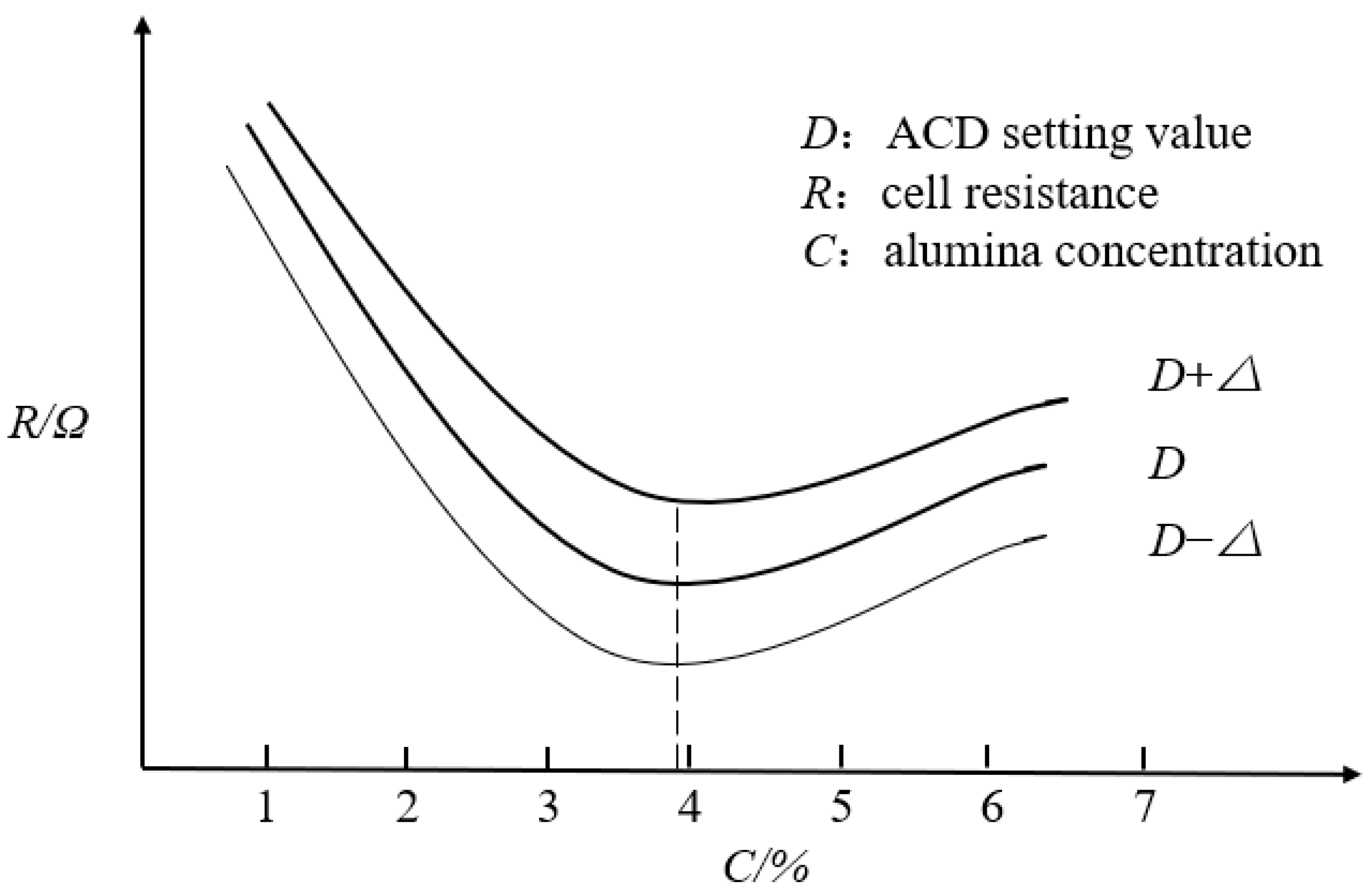
When the cell condition is normal and stable and the change of ACD does not change the shape of the anode bottom, there is a qualitative relationship between cell resistance (apparent), alumina concentration, and ACD [26] as shown in Figure 2. It can be seen from the figure that under the condition of a certain ACD, the relationship between alumina concentration and cell resistance presents a concave curve, and there is an extreme point in the medium alumina concentration area. The theoretical estimation shows that the difference in the set value of ACD mainly affects the height of the relationship curve between the cell resistance and the alumina concentration but has little effect on the shape of the relationship curve [27]. Therefore, the control system can acquire the level of alumina concentration in industrial production by tracking the change of cell resistance in the process of alumina concentration change when ignoring the change of polar distance. The sampling value of the cell resistance can be calculated by the ratio of the cell voltage to the cell current. Considering the actual acquisition of the process data, the bipolar voltage (part of the cell voltage) and the anode current (part of the cell current) are chosen as the auxiliary variables of the alumina concentration.

2.2. Analysis of Different Operating Conditions

In the production process of the aluminum electrolysis industry, some operations are repeated periodically. The analysis of several special conditions is given below.

2.2.1. Anode Effect

Anode effect is a special phenomenon when carbon anode is used in electrolysis. Under the conditions of the cryolite alumina melt electrolysis and carbon anode used, the anodic effect occurs only when the concentration of aluminum oxide in the electrolyte decreases to a certain limit.
The appearance characteristics of the anode effect are described as follows.
(1)
Bright with special sounds and creaks, sparks occur around the anode.
(2)
Bubbles on the anode and electrolyte interface no longer precipitate, and electrolyte stops boiling.
(3)
Fluorocarbon gases are emitted, except for CO and CO2.
(4)
In the industrial electrolytic cell, the voltage rises when the anode effect occurs (generally 30–50 V, individual up to 120 V), and the low-voltage bulb in parallel with the electrolytic cell is shining. Under high-voltage and high-current density, the electrolyte and anode are overheated, and under constant-voltage supply, the series current of the electrolytic cell decreases sharply when the anode effect occurs.
The field characteristics in the cell under anode effect are as follows.
(1)
Reduction in alumina concentration in electrolyte.
(2)
The concentration of the F ion near the carbon anode increased, while the concentration of the oxygen-containing ion decreased.
(3)
The carbon anode potential increased to the F ion discharge potential, and the carbon fluoride gas was precipitated, the anode surface was covered by a gas film.
Based on the above analysis, it can be seen that the occurrence of the anode effect in the industrial electrolytic cell production conditions is a very complex process. In the process of the anode effect occurrence, the process of taking corresponding measures to extinguish the anode effect and the process of extinguishing the anode effect returning to normal production, there may be varying degrees of noise in the collected data.

2.2.2. Anode Changing

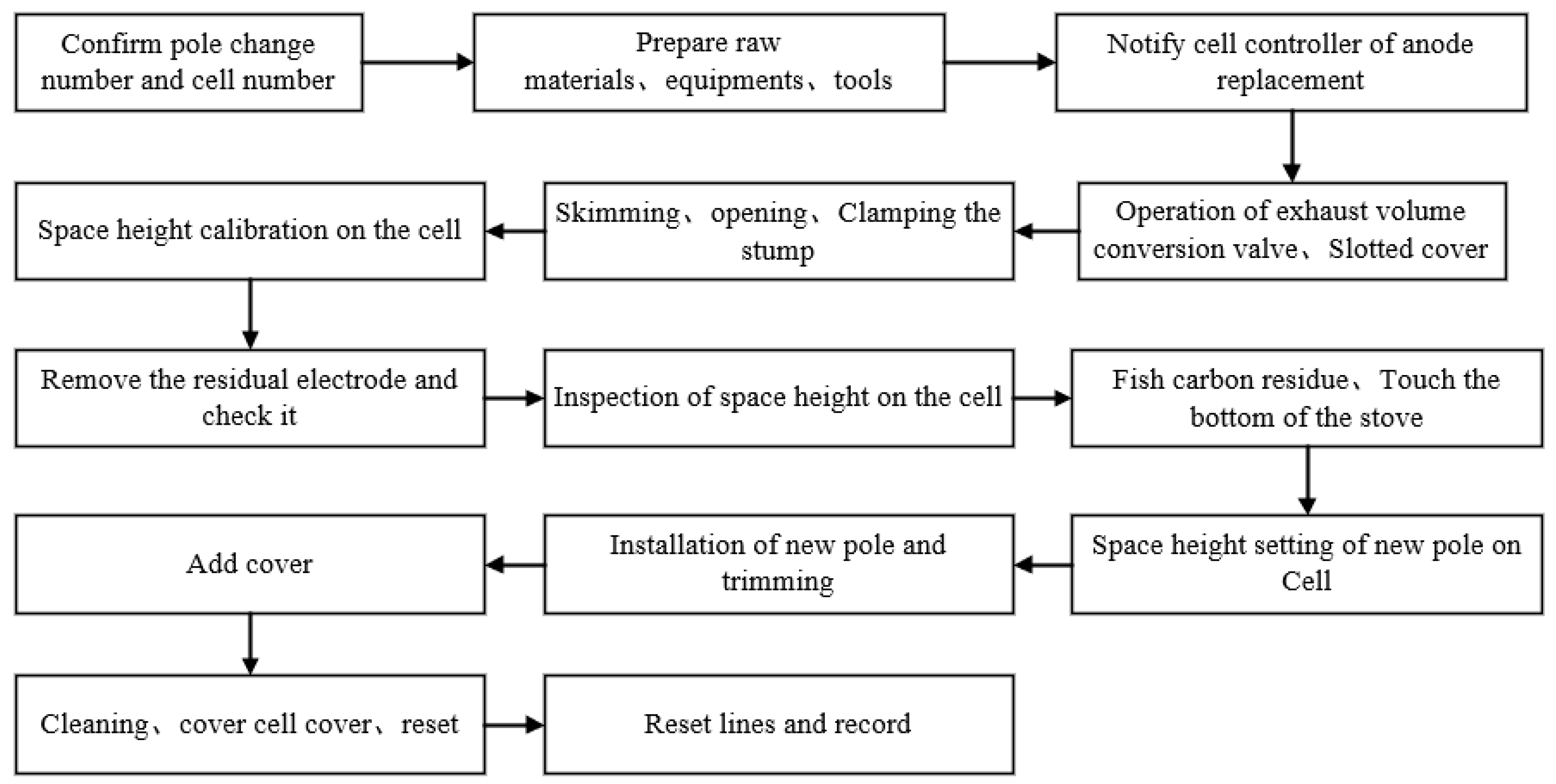
The anode used in the prebaked cell is sent to the electrolysis process after forming, roasting, and assembling the anode rod according to the specified size in the anode factory. After each anode is used for a certain number of days, it is necessary to replace the residual anode and reinstall the new anode, which is the anode changing. The anode changing operates in accordance with a certain cycle. The anode changing process is shown in Figure 3.
Before the anode replacement, the cell controller will be notified and enter the monitoring program of the anode changing. In the process of anode changing, the cell voltage rises slightly when the residual anode is removed. Under the monitoring program of anode changing, the cell controller monitors the change of the cell voltage.

2.2.3. Aluminum Tapping

The aluminum liquid produced by electrolysis is deposited at the bottom of the furnace, which needs to be extracted regularly and sent to the cast factory for casting. Small and medium-sized electrolytic cells usually produce aluminum once in 2~3 days, and large prebaked cells are once a day. The aluminum production process is shown in Figure 4.
Before the aluminum production operation, the cell controller will be notified and enters the aluminum monitoring program. A series of conventional operations such as feeding and aluminum tapping will cause certain noise and fluctuation in process data.

3. Principle of Improved Method

In the process of complex aluminum electrolysis industrial production, different operation conditions have different effects: On the one hand, there is noise in the parameter data of the industrial production process; on the other hand, a specific soft-sensing model of alumina concentration has certain structural limitations. In order to solve this problem, a soft-sensing model of alumina concentration based on EMD–PSO–DBN which combines the EMD algorithm with the PSO algorithm and the DBN soft-sensing model is designed and predict the alumina concentration under the background of the aluminum electrolysis industrial production.

3.1. Empirical Mode Decomposition

Empirical Mode Decomposition (EMD) is a data-processing method for non-stationary and nonlinear time series, which was proposed in [28]. Recently, EMD-based multi-algorithm combination model [29] was developed. The essence of EMD is to decompose the original sequence into several intrinsic mode functions (IMFs) and residual components. Each IMF component contains local characteristic signals at different time characteristic scales of the original signal. At any time, any signal is composed of several IMFs, and the residual component can reflect the slow change of the original signal.
The main calculation process of EMD is as follows:
(1)
Calculate the maximum and minimum values of the original time series x(t) and use the cubic spline curve to fit the upper and lower envelopes of the maximum and minimum values, respectively; the average value of the upper and lower extreme value envelopes is the mean line of the original time series.
(2)
Subtract the mean line from the original time series to check whether the remaining items are stationary and satisfy the IMF condition. Each IMF should satisfy the following two conditions: the numbers of local extreme points and zero-crossing points of the function are equal or at most one difference within the entire data sequence. For any point, the average envelope of local maximum (upper envelope) and local minimum (lower envelope) is 0. If the remaining items do not meet the IMF conditions, repeat the above process until the IMF components that meet the conditions are selected.
Let the mean value of the upper and lower envelopes be m ( t ) , calculate h ( t ) = x ( t ) m ( t ) , and determine whether h ( t ) satisfies the IMF condition. If not, consider h ( t ) as a new x ( t ) and repeat the above operation.
h k ( t ) = h k 1 ( t ) m ( t )
where the h k ( t ) —the k-th calculation results in subtract m(t); m ( t ) —the mean value of the upper and lower envelopes of the original time series x(t).
Until h k ( t ) satisfies the IMF condition, the first IMF is obtained, that is c 1 ( t ) and the residual component r 1 ( t ) of the signal. ( c 1 ( t ) = h k ( t ) )
r 1 ( t ) = x ( t ) c 1 ( t )
where c 1 ( t ) —the first component of the original time series x(t); r 1 ( t ) —Residual component of signal, equal to the first remaining component of the subtracted the first component from the original sequence.
(3)
The above Equation (3) subtracts the selected IMF components from the original sequence and repeats the above process for the remaining sequences until all the IMF components are selected.
(4)
When the original sequence cannot continue to decompose more IMF components and becomes a monotonic function, the final residual part is the trend term of the entire sequence, which is commonly expressed by R E S .
R E S = r n 1 ( t ) c n ( t )
where RES—the final residual component.
By EMD method, the original time series x ( t ) can be expressed as Formula (5).
x ( t ) = i = 1 n I M F i + R E S
where I M F i —the i-th IMF component.

3.2. Optimized the Number of Hidden Layer Nodes by Particle Swarm Optimization

Particle swarm optimization (PSO) is an optimization algorithm developed based on the research of bird predation behavior [30]. Firstly, a particle swarm is randomly initialized, and each particle may be the optimal solution of the solution space. And then calculate the fitness function of each particle, update the particle attributes by comparing the fitness value with the extreme point. Finally, push the particle toward the individual iterates in the direction of the optimal value and the group optimal value until the global optimal value is reached. At present, particle swarm optimization is widely used in many practical problems, including multi-objective optimization [31], signal processing, and neural network training [32]. Based on the design of the DBN soft-sensing model, this paper introduces the PSO algorithm, which combines the PSO with the DBN network. It has the advantages of the PSO algorithm’s fast convergence speed, high robustness, strong global search ability, and does not require the characteristic information of the problem itself.
For the PSO algorithm optimization problem, the solution to be solved corresponds to the particles in the biological population. Firstly, it needs to initialize a particle in the solution space and a random particle in the search space, which constitute a population X = { X 1 , X 2 , X a } . The specific position is   X i = { x i 1 , x i 2 X i n } . The solution space corresponds to the position of each particle, and the fitness of each particle in the particle swarm is solved by the set objective function. Then, each particle is iteratively solved on its location, and the velocity V i = { v i 1 , v i 2 v i n } is constantly updated to search for new solutions. In the process of solving, the PSO algorithm continuously optimizes and adjusts according to two extreme values: the individual extreme value corresponds to P i d , and the global extreme value corresponds to P g d . After the above two extremums are found, the particles iterative speed and position can be represented with the following two formulas (6) and (7), respectively.
v i d k + 1 = w v i d k + c 1 r 1 ( p i d k x i d k ) + c 2 r 2 ( p g d k x g d k )
x i d k + 1 = v i d k + 1 + x i d k
where v i d k + 1 —the speed of the i-th particle in the d-dimension after the k + 1-th iteration; x i d k + 1 —the position of the i-th particle in the d-dimension after the k + 1-th iteration; w -weight; c 1 , c 2 —the acceleration constants; r 1 , r 2 —the random number range [0,1].
The particle velocity should keep a certain constraint on the upper and lower limits to ensure that the particle swarm algorithm can be within the effective speed, as shown in the following formula.
v i d k + 1 = { v m a x   v i d k + 1 > v m a x   v m i n   v i d k + 1 < v m i n    
where v m a x —the upper limit of particle velocity; v m i n —the lower limit of particle velocity.
The particle fitness (mean variance) is
f i t n e s s = 1 n i = 1 n j = 1 c ( Y i j y i j ) 2
where n—the sample number; c—the number of neural network outputs; Y i j j the expected values of sample i; y i j j the actual values of sample i.
The inertia factor w in the PSO algorithm has a great influence on the performance of the algorithm. In the iterative process, the calculation process is easy to fall into the local extremum point. In order to overcome this difficulty, the nonlinear inertia weight is introduced:
w ( t ) = w m i n + ( w m a x w m i n ) e x p [ k ( t t m a x ) 2 ]
where w m a x —the maximum value of inertia weight; w m i n —the minimum value of inertia weight; t —the iterative times; t m a x —the maximum iterations.
From the above analysis, it can be seen that there are three major parts that play a decisive role in the adjustment of velocity and position in the particle iteration process, namely, the original velocity v i d of the particle, the optimal position p g d x g d k of the population, and the optimal position distance p i d x i d k .
There are three important parameters in the particle swarm optimization algorithm, namely w , c 1 and c 2 . w keeps the particles in the motion inertia, and c 1 and c 2 are the weights when the particles accelerate to the individual and global optimal position. If w = 0, the speed of the particle swarm has no memory; the particle swarm converges to the global optimal position, and it cannot search the optimal solution. If c 1 = 0, the particle swarm has no cognitive ability, the convergence speed is accelerated, and it is easy to fall into the local minimum problem. If c 2 = 0, the particle swarm has no group ability, which is equivalent to the particle swarm in independent search, and it is difficult to find the optimal solution.
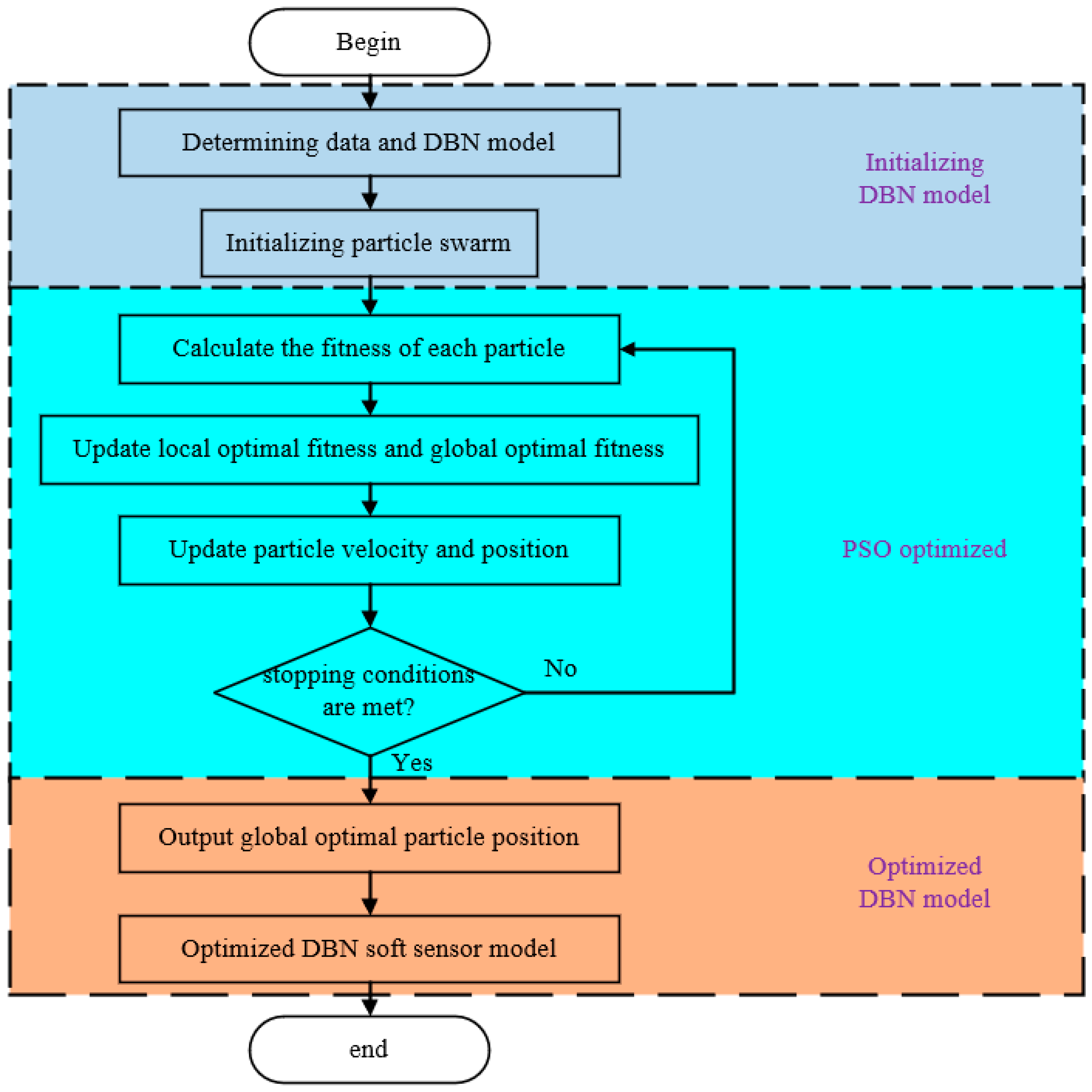
The specific process of the PSO to optimize the DBN model is shown in Figure 5.

3.3. Design of Soft-Sensing Model

Although the alumina soft-sensor model based on the DBN can achieve accurate estimation of alumina concentration to a certain extent, due to the structural characteristics of the DBN, the number of hidden layer nodes in RBM has a certain impact on the training speed and prediction accuracy of the network. The number of hidden layer nodes of the different DBN models is often determined by experience and experimental methods. Therefore, the PSO optimization algorithm is introduced to optimize the number of the RBM hidden layer nodes in each layer of the DBN structure. It can not only improve the accuracy of the soft-sensor model, but also improve the universality of the model under different working conditions.
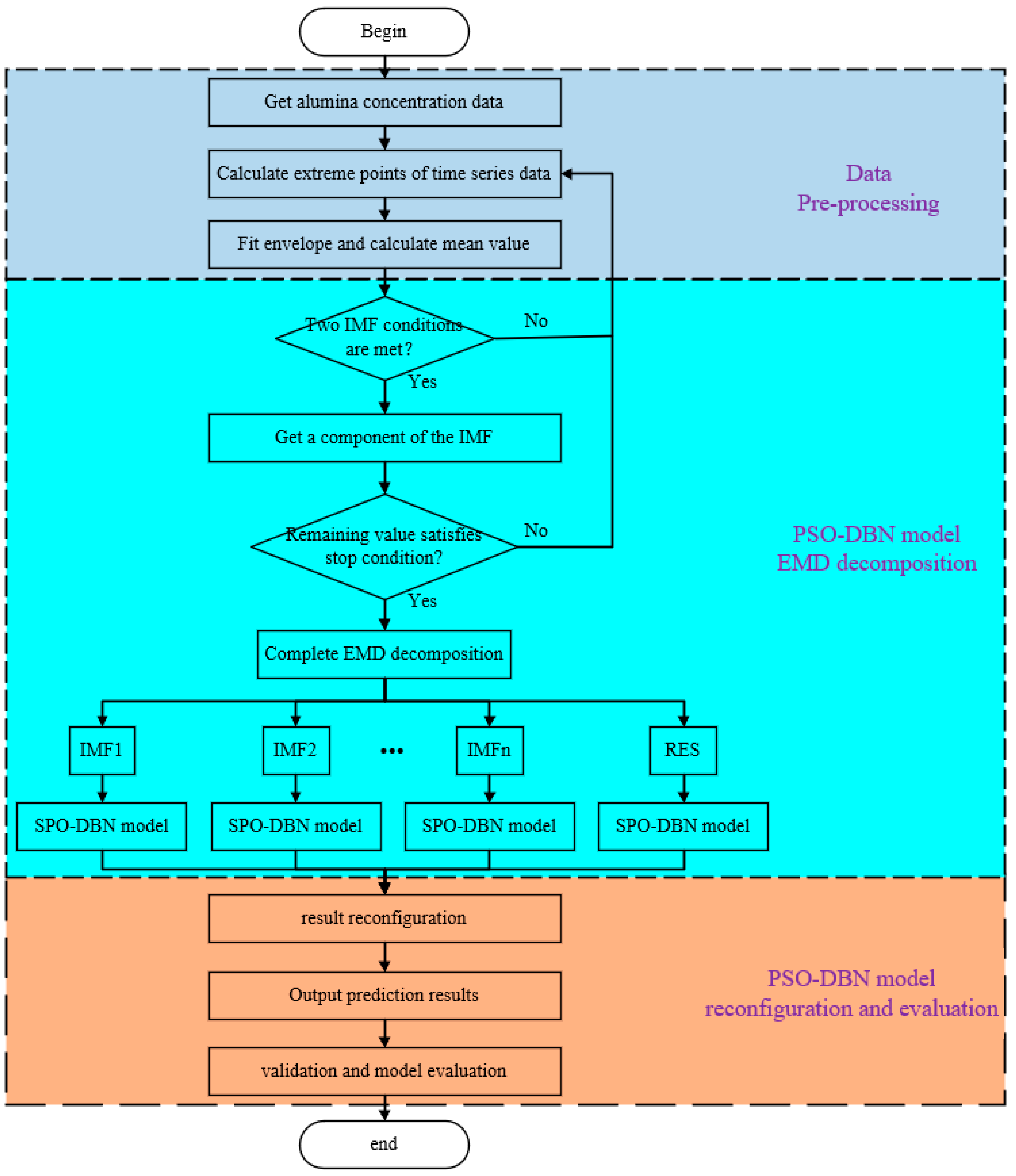
The training of EMD–PSO–DBN is actually the soft-sensor modeling of PSO–DBN with different decomposition modes after the EMD decomposition of the sample data, and the structure of the DBN network is optimized by using the PSO algorithm. The empirical mode decomposition principle in the previous chapter is combined with the PSO-optimized DBN model to complete the soft-sensor training process of EMD–PSO–DBN. The flow chart of soft-sensor model design based on EMD–PSO–DBN is shown in Figure 6.

4. Experiment and Results

In order to verify the effectiveness and accuracy of the improved soft-sensing model of the alumina concentration, the verification analysis is carried out with the production process data of the aluminum electrolysis industry of the Zunyi Aluminum Factory. The data acquisition process, experimental simulation results, and result analysis are as follows.

4.1. Data Acquisition

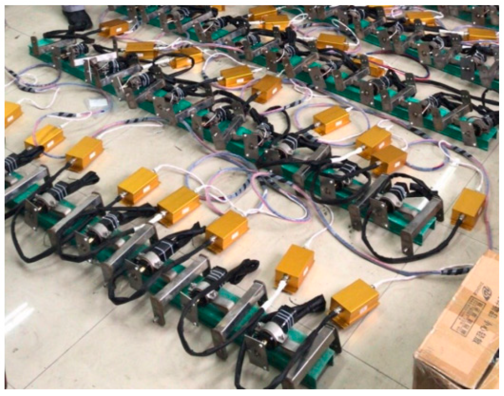
According to the above analysis, it is necessary to collect the main variable data of the alumina concentration and the auxiliary variable data of the corresponding two-pole voltage and anode current. The experimental data is collected from the A side of the No. 2875 electrolytic cell in the Zunyi Aluminum Factory. There are 24 anode rods on the A side, and each anode rod is equipped with an anode rod measuring device to collect the voltage data and current data. A picture of the anode rod measuring device is shown in Figure 7.
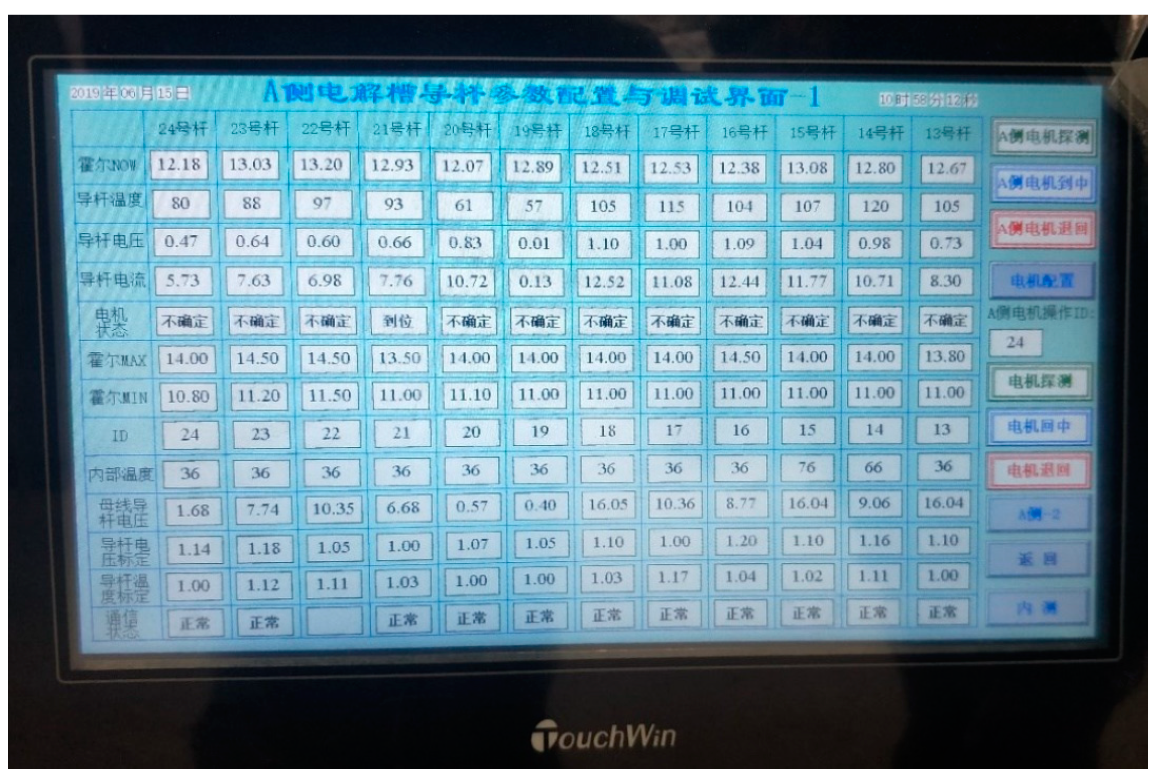
The anode rod measuring device uses the RS485 communication mode to communicate with the host computer to complete the data transmission, and the data are also displayed in the field screen. The data collected in real time are shown in Figure 8.
At present, due to the high temperature, high magnetic, strong coupling environment and complex process flow, there is no alumina concentration sensor that meets the requirements in actual production. The alumina concentration data can only be obtained by on-site sampling and laboratory testing, as shown in Figure 9. The whole measurement process includes drill sampling holes, sampling, cooling the samples, bagging, and sending the samples to the laboratory for assay and analysis.
After data collection and data preprocessing, 600 sets of complete data are selected for analysis, including 500 sets of data for training and 100 sets of data for testing.

4.2. Simulation Experiment

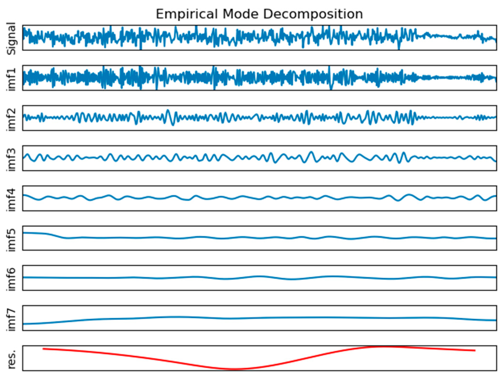
Firstly, the original sequence is decomposed by the EMD method, a total of 7 IMF components and a RES-trend component are obtained, as shown in Figure 10. It can be seen from Figure 10 that the frequency of each IMF component decreases sequentially from high to low. According to the frequency of each IMF component, the IMF1, IMF2, and IMF3 are classified as high-frequency components, and the IMF4, IMF5, IMF6, and IMF7 are classified as low-frequency components. The high-frequency, low-frequency and RES-trend component are established, respectively, based on the PSO–DBN soft-sensing model, and finally the high-frequency, low-frequency and RES-trend component are superimposed to obtain the final alumina concentration prediction value.
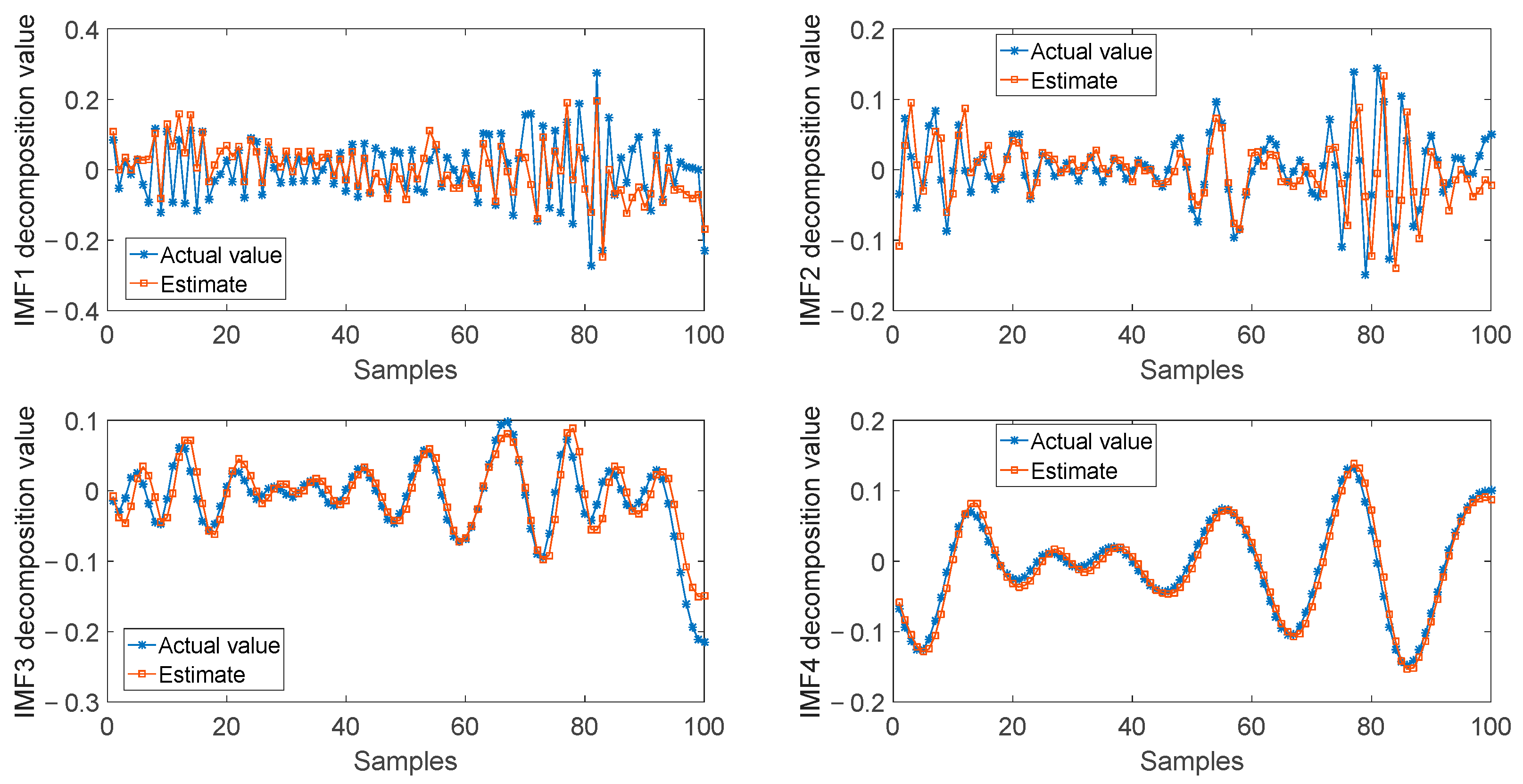
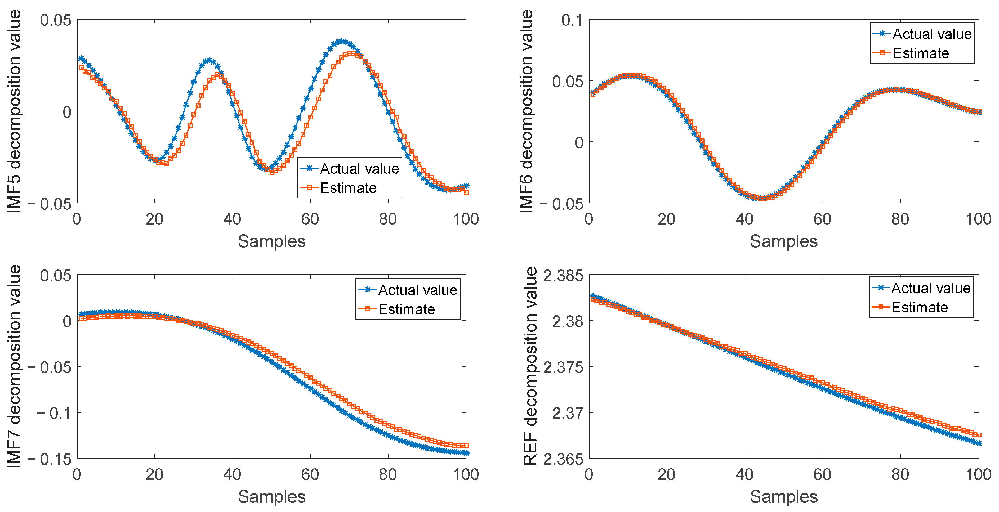
The soft-sensing models based on PSO–DBN are established for high-frequency, low-frequency and RES-trend component, respectively, and finally the RES prediction results of the high-frequency, low-frequency and trend component are reconstructed. The soft-sensing model prediction results of the IMF1, IMF2, IMF3 and IMF4 components are shown in Figure 11, and the prediction results of the IMF5, IMF6, IMF7 and REF components are shown in Figure 12. It can be seen from Figure 11 and Figure 12 that the overall trend-prediction effect for the change of the characteristic components and trend component at different times is relatively good, especially for the prediction of the low-frequency components, which is almost consistent with the actual data after decomposition, but the prediction effect for the high-frequency components is general.
The evaluation indexes of the comparison between the predicted value and the actual value of the corresponding components of the soft-sensing model of PSO–DBN corresponding to each IMF component and REF trend component are shown in Table 1, and the number of hidden layer nodes optimized by the PSO algorithm is given too.
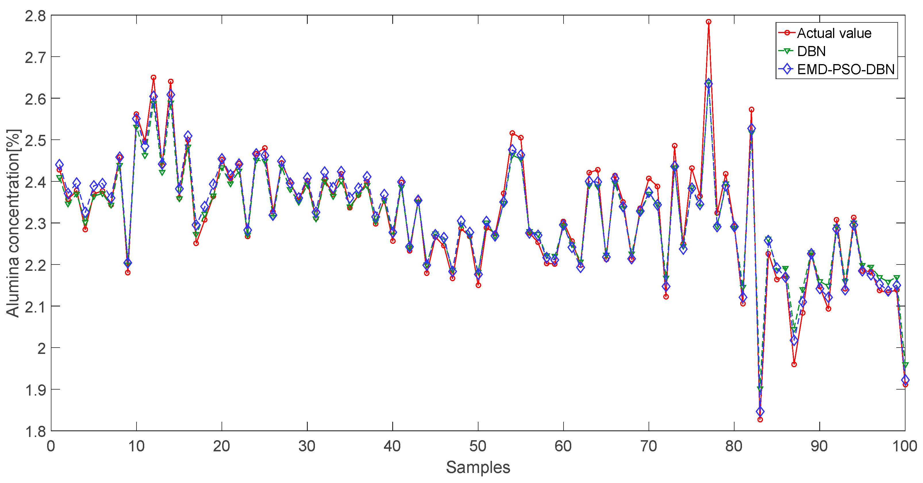
The predicted values of the soft-sensing model established by each IMF component are reconstructed to obtain the final predicted value of the alumina concentration. The comparison between the predicted value and the actual value is shown in Figure 13. Compared with the soft-sensing model of the alumina concentration based on the DBN, it can be seen that the predicted value of the improved soft-sensing model is closer to the actual value, which improves the prediction accuracy of the model.
Table 2 shows the data of the corresponding evaluation indexes of the two models. The goodness of fit of the two soft-sensing models of the alumina concentration is above 0.9, which indicates that the models can accurately follow the change trend of the alumina concentration. The MAE and RMSE values of the EMD–PSO–DBN soft-sensing model are lower than those of the DBN soft-sensing model of alumina concentration, which confirms that the prediction accuracy of soft-sensing model based on EMD–PSO–DBN is higher than the DBN soft-sensing model and proves that the designed method is more suitable for soft-sensing of the alumina concentration.

5. Conclusions

In this work, under multiple working conditions of complex industrial production process, a soft-sensing model of the industrial process based on EMD–PSO–DBN is proposed to solve the problem of data noise and the limitation of the DBN soft-measurement model. First, the complex current sequence is decomposed into the IMF components with eight feature scales by using the EMD algorithm, so as to isolate the mutual influence of different components and achieve the purpose of removing noise. Then, in different electrolytic cells or different operating conditions of the same electrolytic cell, the PSO algorithm is combined with the DBN model to optimize the structure of the number of hidden layer nodes of the soft-sensing model to improve the accuracy and universality of the soft-sensing model. The proposed method is applied to the soft measurement of the alumina concentration in the electrolytic aluminum production process; the results show that the soft-sensing model based on EMD–PSO–DBN can effectively eliminate the influence of noise and optimize the structure of the soft-sensing model. Because the prediction accuracy of soft-sensing model based on EMD–PSO–DBN is higher than the DBN soft-sensing model, it is more suitable for soft sensing of the alumina concentration in the aluminum electrolysis process.
At present, some achievements have been made in the research on the soft sensing of the alumina concentration, but there are still some limitations. The current research mainly focuses on the average alumina concentration of the whole cell, while for large aluminum reduction cells, the significance of the distributed alumina concentration measurement is greater than the average alumina concentration. Therefore, the future work is to establish a distributed alumina concentration soft-sensing model for the distributed current to realize the accurate prediction of the distributed alumina concentration. By combining the intelligent control methods, its purpose is to realize the precise control of the alumina concentration in the whole cell and the refined management of the aluminum reduction cell.

Author Contributions

Conceptualization, X.L. and B.L.; methodology, J.C.; software, W.Q.; validation, X.L.; formal analysis, B.L.; investigation, L.C.; resources, X.L.; data curation, G.R.; writing—original draft preparation, X.L.; writing—review and editing, X.L.; visualization, B.L.; supervision, B.L.; project administration, J.C.; funding acquisition, X.L. All authors have read and agreed to the published version of the manuscript.

Funding

This research was funded by the Science and Technology Project of Jiangxi Provincial Department of Education, China, grant number GJJ151276; funded by the Industrial Project of Jingdezhen Science and Technology Bureau, China, grant number 2016GYZD012-04; and it was also funded by the Science and Technology Project of Jiangxi Provincial Department of Education, China, grant number GJJ191173.

Data Availability Statement

The data comes from the actual industrial aluminum factory. We have signed an agreement with the enterprise. The relevant data are confidential, so the data set used in this paper cannot be disclosed.

Conflicts of Interest

The authors declare no conflict of interest.

References

  1. Tian, Z.D.; Li, S.J.; Wang, Y.H.; Sha, Y. A prediction method based on wavelet transform and multiple models fusion for chaotic time series. Chaos Solitons Fractals 2017, 98, 158–172. [Google Scholar]
  2. Guo, D.P.; Zhou, P. Soft-sensor modeling of silicon content in hot metal based on sparse robust LS-SVR and multi-objective optimization. Chin. J. Eng. 2016, 38, 1233–1241. [Google Scholar]
  3. Zhou, Y.; Yang, J.S.; Fu, D.M.; Yue, B. BCOISOA-BP network in grinding particle size soft sensor applications. Chin. J. Eng. 2017, 39, 1546–1551. [Google Scholar]
  4. Gao, J.; Yang, X.; Huang, J.; Peng, K. A data-driven fault detection and fault-tolerant control scheme for large-scale systems and its application on multi-area interconnected power systems. IET Control Theory Appl. 2022. [Google Scholar] [CrossRef]
  5. Huang, J.; Yang, X.; Peng, K. Double-Layer Distributed Monitoring Based on Sequential Correlation Information for Large-Scale Industrial Processes in Dynamic and Static States. IEEE Trans. Ind. Inform. 2020, 17, 6419–6428. [Google Scholar] [CrossRef]
  6. Sun, Q.; Ge, Z. A Survey on Deep Learning for Data-Driven Soft Sensors. IEEE Trans. Ind. Inform. 2021, 17, 5853–5866. [Google Scholar] [CrossRef]
  7. Ke, W.; Huang, D.; Yang, F.; Jiang, Y. Soft sensor development and applications based on LSTM in deep neural networks. In Proceedings of the 2017 IEEE Symposium Series on Computational Intelligence (SSCI), Honolulu, HI, USA, 27 November–1 December 2017; pp. 1–6. [Google Scholar] [CrossRef]
  8. Yuan, X.; Li, L.; Wang, Y. Nonlinear Dynamic Soft Sensor Modeling with Supervised Long Short-Term Memory Network. IEEE Trans. Ind. Inform. 2019, 16, 3168–3176. [Google Scholar] [CrossRef]
  9. Curreri, F.; Patanè, L.; Xibilia, M.G. Soft Sensor Transferability: A Survey. Appl. Sci. 2021, 11, 7710. [Google Scholar] [CrossRef]
  10. Alakent, B. Soft sensor design using transductive moving window learner. Comput. Chem. Eng. 2020, 140, 106941. [Google Scholar] [CrossRef]
  11. Alakent, B. Soft-sensor design via task transferred just-in-time-learning coupled transductive moving window learner. J. Process Control 2021, 101, 52–67. [Google Scholar] [CrossRef]
  12. Farahani, H.S.; Fatehi, A.; Nadali, A.; Shoorehdeli, M.A. Domain Adversarial Neural Network Regression to design transferable soft sensor in a power plant. Comput. Ind. 2021, 132, 103489. [Google Scholar] [CrossRef]
  13. Liu, Y.; Yang, C.; Liu, K.; Chen, B.; Yao, Y. Domain adaptation transfer learning soft sensor for product quality prediction. Chemom. Intell. Lab. Syst. 2019, 192, 103813. [Google Scholar] [CrossRef]
  14. Graziani, S.; Xibilia, M.G. Improving Soft Sensors performance in the presence of small datasets by data selection. In Proceedings of the 2020 IEEE International Instrumentation and Measurement Technology Conference (I2MTC), Dubrovnik, Croatia, 25–28 May 2020; pp. 1–6. [Google Scholar]
  15. Hsiao, Y.-D.; Kang, J.-L.; Wong, D. Development of Robust and Physically Interpretable Soft Sensor for Industrial Distillation Column Using Transfer Learning with Small Datasets. Processes 2021, 9, 667. [Google Scholar] [CrossRef]
  16. Zhang, S.; Zhang, T.; Yin, Y.; Xiao, W. Alumina Concentration Detection Based on the Kernel Extreme Learning Machine. Sensors 2017, 17, 2002. [Google Scholar] [CrossRef] [PubMed] [Green Version]
  17. Zhang, S.; Chen, X.; Yin, Y. An ELM Based Online Soft Sensing Approach for Alumina Concentration Detection. Math. Probl. Eng. 2015, 2015, 268132. [Google Scholar] [CrossRef] [Green Version]
  18. Cui, J.R.; Zhang, N.N.; Yang, X. Soft sensing of alumina concentration in aluminum electrolysis industry based on deep belief network. In Proceedings of the 2020 Chinese Automation Congress (CAC), Shanghai, China, 6–8 November 2020. [Google Scholar]
  19. Zhang, Y.; Yang, X.; Shardt, Y.A.W.; Cui, J.; Tong, C. A KPI-Based Probabilistic Soft Sensor Development Approach that Maximizes the Coefficient of Determination. Sensors 2018, 18, 3058. [Google Scholar] [CrossRef] [Green Version]
  20. Li, J.; Wang, W.; Chen, G.; Han, Z. Spatiotemporal assessment of landslide susceptibility in Southern Sichuan, China using SA-DBN, PSO-DBN and SSA-DBN models compared with DBN model. Adv. Space Res. 2022, 69, 3071–3087. [Google Scholar] [CrossRef]
  21. Huang, N.E.; Shen, Z.; Long, S.R.; Wu, M.C.; Shih, H.H.; Zheng, Q.; Yen, N.-C.; Tung, C.C.; Liu, H.H. The empirical mode decomposition and the Hilbert spectrum for nonlinear and non-stationary time series analysis. Proc. R. Soc. Lond. Ser. A Math. Phys. Eng. Sci. 1998, 454, 903–995. [Google Scholar] [CrossRef]
  22. Zhang, X.H.; Feng, A.M. Short-term traffic flow prediction based on empirical mode decomposition and long short-term memory neural network. J. Comput. Appl. 2021, 41, 225–230. [Google Scholar]
  23. Meng, X.Y.; Wang, R.H.; Zhang, X.P.; Wang, M.J.; Qiu, G.; Wang, Z.X. Ultra-short-term wind power prediction based on empirical mode decomposition and multi-branch neural network. J. Comput. Appl. 2021, 41, 237–242. [Google Scholar]
  24. Xie, H. Prediction of Driving Condition for Plug-In Hybrid Electric Vehicles; Chongqing University: Chongqing, China, 2014. [Google Scholar]
  25. Shi, B.; Li, Y.X.; Yu, X.H.; Yan, W. Short-term load forecasting based on modified particle swarm optimizer and fuzzy neural network model. Syst. Eng. Theory Pract. 2010, 30, 157–166. [Google Scholar]
  26. Liu, Y.X.; Li, J. Modern Aluminum Electrolysis; Metallurgical Industry Press: Beijing, China, 2008. [Google Scholar]
  27. Tessier, J.; Gary, P.T.; Batista, E. Towards on-line monitoring of alumina properties at a pot level. In Light Metal; Springer: Cham, Switzerland, 2012; pp. 633–638. [Google Scholar]
  28. Haupin, W.E. Production of Aluminum and Alumina; John Wiley & Sons: Chichester, UK, 1987. [Google Scholar]
  29. Cao, Y.; Liu, S.; Cao, X.; Liu, X.; Hu, H.; Zhang, T.; Yu, L. EMD-based multi-algorithm combination model of variable weights for oil well production forecast. Energy Rep. 2022, 8, 13389–13398. [Google Scholar] [CrossRef]
  30. Shi, Y.H.; Eberhart, R.C. Empirical study of particle swarm optimization. In Proceedings of the 1999 Congress on Evolutionary Computation-CEC99 (Cat. No. 99TH8406), Washington, DC, USA, 6–9 July 1999; IEEE: New York, NY, USA, 1999; Volume 3, pp. 1945–1950. [Google Scholar]
  31. Zhu, W.; Rad, H.N.; Hasanipanah, M. A chaos recurrent ANFIS optimized by PSO to predict ground vibration generated in rock blasting. Appl. Soft Comput. 2021, 108, 107434. [Google Scholar] [CrossRef]
  32. Zhang, J.R.; Zhang, J.; Lok, T.M.; Lyu, M.R. A hybrid particle swarm optimization-back-propagation algorithm for feedforward neural network training. Appl. Math. Comput. 2006, 185, 1026–1037. [Google Scholar] [CrossRef]
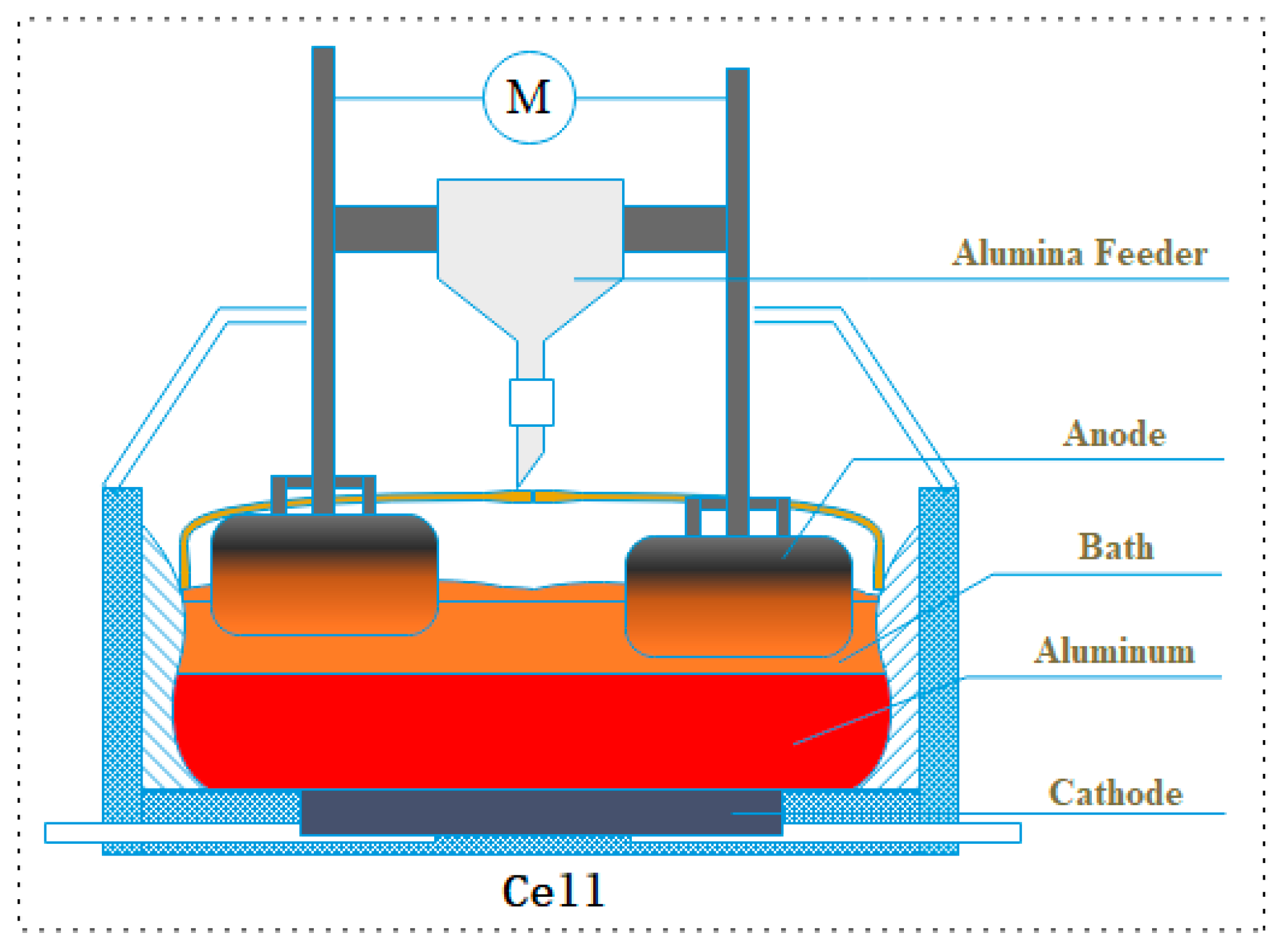
Figure 1. Profile of modern aluminum reduction cell.
Processes 10 02537 g001
Figure 2. Qualitative relation diagram of cell resistance, alumina concentration and ACD.
Processes 10 02537 g002
Figure 3. Flow chart of anode changing operation.
Processes 10 02537 g003
Figure 4. Flow chart of aluminum tapping.
Processes 10 02537 g004
Figure 5. Flow chart of DBN soft-sensing model optimized by PSO.
Processes 10 02537 g005
Figure 6. Flow chart of soft-sensing model based on EMD–PSO–DBN.
Processes 10 02537 g006
Figure 7. Schematic diagram of offline commissioning of anode rod measuring device.
Processes 10 02537 g007
Figure 8. Data acquisition display diagram of anode current measuring device.
Processes 10 02537 g008
Figure 9. The collection process of electrolyte.
Processes 10 02537 g009
Figure 10. The result of EMD decomposition.
Processes 10 02537 g010
Figure 11. The predictive comparison of IMF1, IMF2, IMF3 and IMF4 components.
Processes 10 02537 g011
Figure 12. The predictive comparison of IMF5, IMF6, IMF7 and REF components.
Processes 10 02537 g012
Figure 13. Comparison of prediction and actual value of soft-sensing model for the alumina concentration.
Processes 10 02537 g013
Table 1. Evaluation indexes of soft-sensing models for IMF components.
ComponentsNumber of Hidden LayersMAERMSER2
IMF124–280.05360.06770.6877
IMF250–310.03010.04260.5932
IMF336–450.01820.02380.9039
IMF419–200.01030.01220.9844
IMF533–350.00630.00800.9548
IMF641–530.00170.00210.9981
IMF736–200.00720.00830.9979
REF21–230.00050.00050.9950
Table 2. Comparison of soft-sensing model in the test set.
MethodsMAERMSER2
DBN0.02190.03060.9950
EMD–PSO–DBN0.01840.02590.9881
Publisher’s Note: MDPI stays neutral with regard to jurisdictional claims in published maps and institutional affiliations.