Optimum Power Flow with Respect to the Capacitor Location and Size in Distribution Network

Abstract

In the past few decades, there has been increasing recognition of the importance of optimum power flow (OPF) studies in the context of economic analyses of power systems. There is a need for power system development to maximize efficiency by emphasizing cost and power losses for smart grids to operate effectively in the current situation. This study aims to develop an optimal capacitor bank allocation schedule that minimizes power losses in the distribution networks under equality constraints. This will be achieved by integrating the loss factor and voltage stability into a new approach to determine where the capacitor banks should be located. It aims to reduce the operating costs of power systems and maximize efficiency by applying an optimization model for economic dispatch, which considers distributed power generation and demand response. The NSGA-II optimization algorithm was used in this study to determine the optimal size and location of the capacitor bank. A NSGA-II solves this problem by minimizing cost and power losses while determining the best operating strategy. We used an IEEE 26-bus distribution system to test the proposed method with every possible generation change. Comparing the power flow analysis with/without capacitor optimization showed that the operation optimization model of OPF with NSGA-II can reduce operation costs and improve the power system.

1. Introduction

Over the last few years, optimal power flow (OPF) has been critical in studying power systems [1]. In OPF, selected objective functions are optimized while meeting equality and inequality constraints. It is non-linear, large-scale, nonconvex, and static programming. A state variable and a control variable represent the inequality constraints in regard to the OPF problem, whereas power balance equations represent the equality constraints in terms of the OPF problem. State variables are determined by evaluating the slack bus, load bus voltage, active and reactive power generation, and apparent power flow on the slack bus. On the other hand, Variables in the control system include active power generation, excluding slack buses, generator bus voltage, tap changer, and shunt compensator reactive power [2,3]. The higher fuel cost in recent years has made it an objective function to optimize the OPF problem since it increases generation costs.

Furthermore, thermal power plant emissions are another concern for power system planning due to their release into the atmosphere [4]. Meanwhile, transmission losses have increased due to insufficient reactive power sources in power systems due to the high electricity demand. The study [5] aims to find OPF for a hybrid energy system and control the network using energy storage. To predict the proposed control system, different objective functions are considered, including charge state, energy source accessibility, and load side power demand. Many studies also investigate other objective functions of emissions and transmission losses [6].

Several traditional optimization techniques have been applied successfully to solve the OPF problem, including non-linear programming, quadratic programming, and the interior point method [4,7]. Although these algorithms are non-linear, they cannot be used in practical systems due to their non-linear characteristics. Because of these non-linear characteristics, solutions may be trapped in local optima, so following these algorithms takes a lot of time and energy. Therefore, many optimization methods need to be improved to overcome these problems. Power systems experts have recently employed several population-based optimization algorithms to solve a complex constrained optimization problem. There are also some other techniques such as differential evolution (D), genetic algorithm(GA), artificial bee colony (ABC), the dragonfly algorithm (DA), particle swarm optimization (PSO), tabu search (TS), ant colony optimization (ACO), and grey wolf optimizer (GWO). In the power system, even if population-based optimization techniques successfully optimize a single objective function, reducing only one objective function is insufficient, as many other problems need to be reduced, including fuel cost, emissions, and transmission losses [8]. As a result, many objective functions need to be taken into consideration. As there are three objective functions in this study (fuel cost, emissions, and transmission losses), there is an infinity of optimal solutions between the objective functions, which are called Pareto optimal solutions [9].

Research on the multi-objective form of OPF has been conducted in several fields. A multi-objective OPF problem with FACTS devices has been explored in [10,11,12], a multi-objective optimal power flow problem considering cost, loss, and voltage deviation index was studied in [6], and an improved strength Pareto evolutionary algorithm was developed in [13] to solve a multi-objective OPF problem considering cost, loss, emissions, and voltage stability. The multi-objective optimization problems have been systematically treated in three different ways in the literature. The first step that can be taken is to reduce the multi-objective problem into a single-objective optimization problem to solve it. Therefore, the main objective is defined as a target, while the others are defined as constraints that limit the main objective. In the second approach, all objective functions are combined into one objective function, and the single-objective optimization process is used. These methods have several problems, such as the limitation of choices and the difficulty of selecting the weighting coefficients. As a third type of approach, decision-making-based methods provide better performance when compared with the other types of approaches mentioned previously.

For the current study, improving the multi-objective algorithm’s search performance for solving OPF problems is necessary. It presents a multiobjective-GA algorithm and evaluates its performance on IEEE 26-bus power systems. Three objective functions-operation costs, power loss, and voltage regulation, with respect to the capacitor size and locations, were considered individually and simultaneously as part of the power flow problem. The following objective considers for the current study:

(1)

To analyze voltage violation for the distribution network before and after the multi-objective algorithm solution (NSGA-ii algorithm).

(2)

To analyze the system’s power loss for the distribution network by comparing the before and after NSGA-II OPF.

(3)

To analyze the power system network by considering the cost of the system with respect to the capacitor location and size.

The rest of the article is classified into four sections as follows. Section 2 introduces the methodology modeling and constraints of the multi-objective optimization, and the IEEE bus network data are explained. Section 3 presents the optimization results and the comparisons between the power flow analysis, economic dispatch, and OPF based on IEEE 26 bus. Finally, in Section 4, the conclusions and discussion of the simulation results of the proposed algorithm are described. These are details about the resistance and inductance of the feeders. Matlab codes were used to simulate the test system. Loads and capacitors are modeled as impedances.

2. Materials and Methods

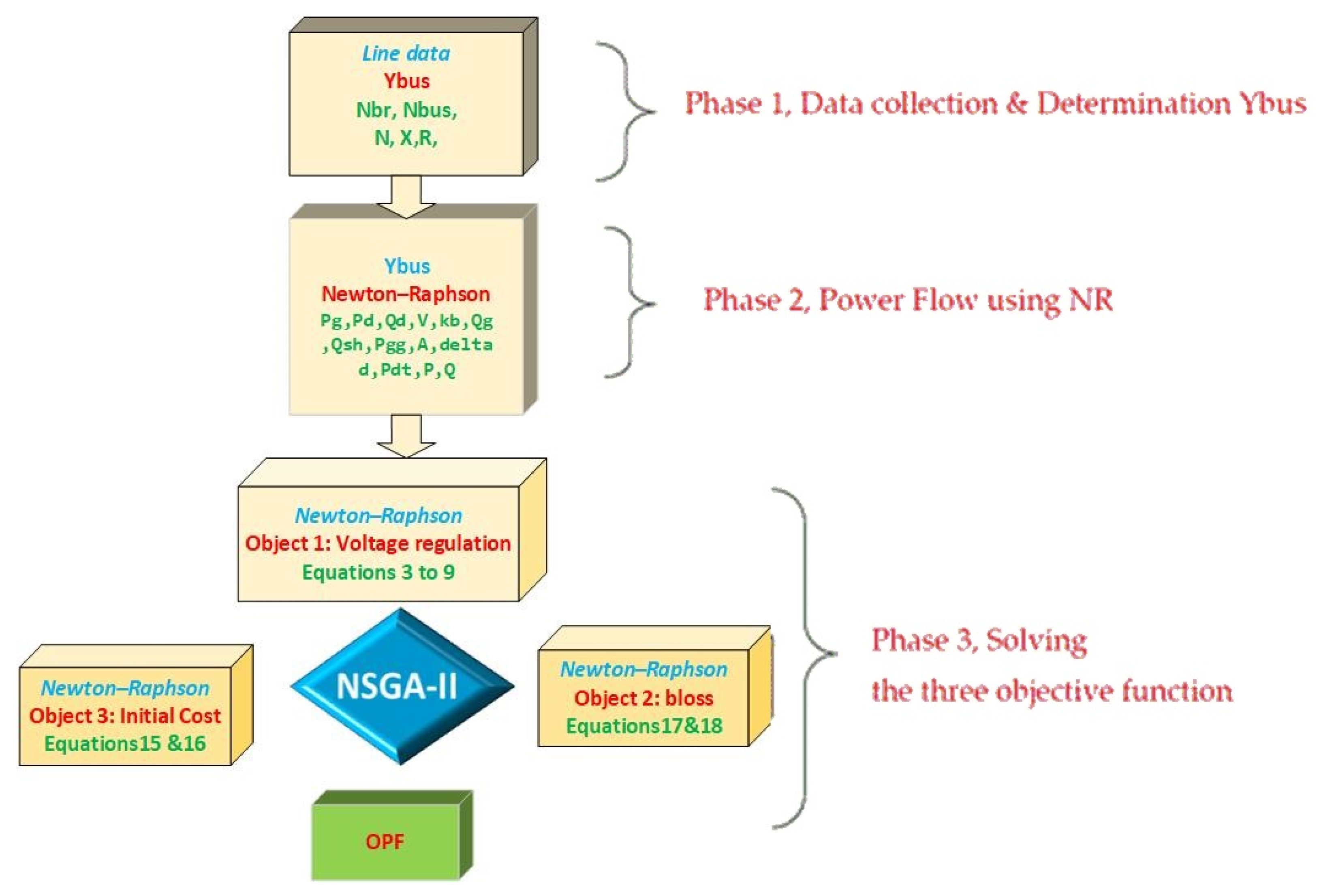
The placement of capacitors is mainly to minimize losses and improve voltage profiles. To accomplish this, an objective function needs to be formulated. Its main goal is to minimize active and reactive power losses while improving voltage profiles [14,15]. A description of the load, network, capacitor, the formulation of constraints, the objective function, and the calculation of power loss can be found in the following section. Generally, this approach is used to optimize total generation costs, emissions generated, and system losses. We are using MATLAB to simulate the IEEE 26 bus system. This study is divided into three phases: network data collection to determine Y bus (Phase 1), power flow analysis using the Newton Raphson technique (Phase 2), and multi-objective variable to find OPF (Phase 3). Figure 1 shows the OPF for the current study by considering three objectives and employing an NSGA-II solver.

2.1. Network Data

A standard IEEE 26 bus test system (

Table A1. Line data for IEEE 26 Bus.

Bus NL	BUS NR	R (PU)	X (PU)	0.5 B (PU)
1	2	0.00055	0.0048	0.03
1	18	0.0013	0.0115	0.06
2	3	0.00146	0.0513	0.05
2	7	0.0103	0.0586	0.018
2	8	0.0074	0.0321	0.039
2	13	0.00357	0.0967	0.025
2	26	0.0323	0.1967	0
3	13	0.0007	0.00548	0.0005
4	8	0.0008	0.024	0.0001
4	12	0.0016	0.0207	0.015
5	6	0.0069	0.03	0.099
6	7	0.00535	0.0306	0.00105
6	11	0.0097	0.057	0.0001
6	18	0.00374	0.0222	0.0012
6	19	0.0035	0.066	0.045
6	21	0.005	0.09	0.0226
7	8	0.0012	0.00693	0.0001
7	9	0.00095	0.0429	0.025
8	12	0.002	0.018	0.02
9	10	0.00104	0.0493	0.001
10	12	0.00247	0.0132	0.01
10	19	0.0547	0.236	0
10	20	0.0066	0.016	0.001
10	22	0.0069	0.0298	0.005
11	25	0.096	0.27	0.01
11	26	0.0165	0.097	0.004
12	14	0.0327	0.0802	0
12	15	0.018	0.0598	0
13	14	0.0046	0.0271	0.001
13	15	0.0116	0.061	0
13	16	0.01793	0.0888	0.001
14	15	0.0069	0.0382	0
15	16	0.0209	0.0512	0
16	17	0.099	0.06	0
16	20	0.0239	0.0585	0
17	18	0.0032	0.06	0.038
17	21	0.229	0.445	0
19	23	0.03	0.131	0
19	24	0.03	0.125	0.002
19	25	0.119	0.2249	0.004
20	21	0.0657	0.157	0
20	22	0.015	0.0366	0
21	24	0.0476	0.151	0
22	23	0.029	0.099	0
22	24	0.031	0.088	0
23	25	0.0987	0.1168	0

) is used to test the proposed algorithm. This system consists of 26 buses and six generators. In Appendix A, we present data on IEEE-26 bus systems. These data include information about load, generators, and bus types and numbers. There are three buses, slack, PV, and PQ, which are determined by 1, 2, and 3, respectively. There are six generators in this network, connected to buses 1, 2, 3, 4, 5 and 26.

Table 1. Generation constraints and cost coefficient.

Generators	Cost Coefficient			Constant Limit
	a	b	c	Min (MW)	Max (MW)
G1	160	9.5	0.007	60	240
G2	176	11	0.009	80	340
G3	156	9.5	0.009	60	240
G4	210	10.5	0.009	80	290
G5	149	10.5	0.008	50	340
G6	170	10	0.007	50	320

has five generators, each with a total generation of 1672 MW. In the following table, the total load demand is 1650 MW with 641 Mvar and capacitor sizes and locations. Information about network lines has been added to Appendix A. There are two equations and four unknowns for each bus, meaning that two variables must be specified for each equation. A bus can be classified into three types, depending on which variables are defined: Load or PQ, PV, Slack Bus. The impedance model of loads and capacitors is described in Equations (1) and (2).

$$Z_{load}=R_{Load}+j{X}_{load}$$

(1)

$$Z_{ck}=-j{X}_{ck}$$

(2)

where Z_load, R_Load and X_load are the impendence of the ith load, the resistance of the ith load and the reactance of the ith load, respectively. Z_ck and X_ck are the impedance of the kth capacitor and the reactance of the kth capacitor. As a result of capacitive impedance, the inductive reaction is canceled, and power network losses are minimized.

2.2. Power Flow Calculation

An electric power system has been designed to be at its steady-state operating point by finding the steady-state operating point of the load flow or power flow. The objective is to obtain all bus voltages and complex power flowing through all network components, including generating units, transmission lines, and loads. Power flow analysis is one of the most widely used tools in electric power systems and can be used either as a stand-alone tool or as part of a more complex process, such as stability analysis and optimization. There are non-linear algebraic equality or inequality constraints that can be defined as part of the solution. It is important to remember that these constraints represent Kirchhoff’s laws and the operational limits of a network. The power flows of transmission lines are considered as follows Eq accordingly. The power system will suffer from excessive capacitive reactive power, leading to a leading power factor and heating losses in the end users’ equipment. For this reason, shunt capacitor banks have to be sized and placed optimally.

$$P_{ij}=|V_i{|}^2{G}_{ij}-\left|V_i\right|\ast \left|V_j\right|\left(G_{ij}\cos {\delta }_{ij}+B_{ij}\sin {\delta }_{ij}\right)$$

(3)

$$Q_{ij}=-|V_i{|}^2{B}_{ij}-\left|V_i\right|\ast \left|V_j\right|\left(G_{ij}\sin {\delta }_{ij}-B_{ij}\cos {\delta }_{ij}\right)$$

(4)

$$P_{ji}=|V_j{|}^2{G}_{ij}-\left|V_i\right|\ast \left|V_j\right|\left(G_{ij}\cos {\delta }_{ij}+B_{ij}\sin {\delta }_{ij}\right)$$

(5)

$$Q_{ji}=|V_j{|}^2{B}_{ij}-\left|V_i\right|\ast \left|V_j\right|\left(G_{ij}\cos {\delta }_{ij}+B_{ij}\cos {\delta }_{ij}\right).$$

(6)

where, $V_i$ and $V_j$ are voltage amplitudes at bus i and bus j, respectively; δ_i, δ_j, and δ_ij are voltage phase angles at busi, busj, and the difference in the voltage angle between buses I and j, respectively; and G_ij and B_ij are defined as (7) & (8)

$$G_{ij}=\frac{R_{ij}}{R_{ij}^2+X_M^2}$$

(7)

$$B_{ij}=\frac{X_N}{R_{ij}^2+X_M^2}$$

(8)

where, R_ij is the resistance of the transmission line between bus i and j; G_ij and B_ij are the conductance and susceptance between bus i and bus j, respectively.

Newton-Raphson Solution Method

Several iterative methods have been employed through the years to solve the power flow problem, but the Newton–Raphson method has proven to be the most effective. This method incrementally improves the unknown values by using first-order approximations of non-linear algebraic equations. A Newton–Raphson method applies quadratically when the initial guess value is close to the solution. Based on the above equations, a linear system of equations can be written as follows:

$$\left(\begin{array}{c}\Delta \theta \\ \Delta V\end{array}\right)=-J{ }^{-1}\left(\begin{array}{c}\Delta P\\ \Delta Q\end{array}\right)$$

(9)

According to the OPF studies, the equality constraints correspond to the topology and structure of the power network. To meet these constraints, the following measures have been taken:

$$\Delta P_P=P_{GI}-P_{Di}-V_i{\displaystyle \sum }_{j=1}^{NB}{V}_j\ast \left(G_{ij}\cos {\delta }_{ij}+B_{ij}\sin {\delta }_{ij}\right)$$

(10)

$$\Delta Q_p=Q_{Gi}-Q_{Di}-V_i{\displaystyle \sum }_{j=1}^{NB}{V}_j\ast \left(G_{ij}\sin {\delta }_{ij}-B_{ij}\cos {\delta }_{ij}\right)$$

(11)

The real and reactive power generations at bus i are indicated by P_GI and Q_Gi, respectively, and the real and reactive power demands at bus i are indicated by P_Di and Q_Di. The number of buses in total is NB. The OPF inequality constraints reflect the physical limits on the devices in the power system as well as the security constraints created by the power system to guarantee its reliability and security. The J is a matrix of partial derivatives known as a Jacobian:

$$J=\left[\begin{array}{cc}\frac{\partial \Delta \theta }{\partial \theta }& \frac{\partial \Delta P}{\partial V}\\ \frac{\partial \Delta Q}{\partial \theta }& \frac{\partial \Delta Q}{\partial V}\end{array}\right]$$

(12)

Solving the linearized system of equations allows one to determine the next guess (m + 1) of voltage magnitude and angle. In this process, the process continues until a stopping condition is met. There is a common stopping condition in which the mismatch equations should be terminated if the norm of the mismatch equations falls below a certain tolerance.

$${\theta }^{m+1}={\theta }^m+\Delta \theta$$

(13)

$$V^{m+1}=V^m+\Delta V$$

(14)

2.3. Multi-Objective Function

It is important to understand that OPFs in power systems are nonconvex, non-linear optimization problems with definite objectives that are reduced under operational inequality and equality constraints. Solving OPF as part of power system studies is an important but challenging task. In addition to optimizing power system performance, the OPF is also responsible for ensuring that equality and inequality constraints are met within the power system. OPF can be solved in various ways depending on the approach that is taken. Several strategies are available, including reducing the total cost of generation, the total emissions, and the total losses in the system. Each of these objectives can be viewed as a single objective function, which can be defined as follows:

$${\mathrm{F}}_2=Min C_{total}={{\displaystyle \sum }}_{i=1}^{NG}{C}_i\left(P_{gi}\right)$$

(15)

$$C_i\left(P_{gi}\right)=a_i+b_i{P}_{gi}+C_i{P}_{gi}^2$$

(16)

In this equation, C_i (P_gi) represents the cost of generation for unit i, P_gi represents the power generated by unit i, and a_i, b_i, c_i represents the cost coefficient for unit i. For the purpose of minimizing the total power system’s energy production cost, the generator cost function was selected. Using this objective function, the OPF reflects the costs of generating power. The number of generation units, or NG, refers to the total number of units within the energy generation system used to minimize the total system cost associated with active power generation, P_gi. A third objective function is to obtain a minimum amount of total losses during the power system operation by obtaining a minimum amount of total losses. This equation gives the complex power at the ith bus according to Equation (17):

$${\mathrm{F}}_3=Min T_{loss}={{\displaystyle \sum }}_{i=1}^{NG}{P}_{gi}-P_{load}$$

(17)

$$P_i-j{Q}_i=V_i\ast I_i$$

(18)

The term T_loss refers to the sum of system losses, P_gi refers to the power generated by unit 1, and P_load refers to the combined load in the system. P_i, Q_i, V_i, and I_i are active power, reactive power, voltage, and current, respectively. According to the OPF equality constraints, the desired voltage set points throughout the power system are determined by the physics of the power system. Several physical devices require the enforcement of limits. These include generators, tap-changing transformers, and phase-shifting transformers. As shown in Table 1, there are constraints on how each generation of units can be operated for the current study. In OPF studies, inequality limitations and constraints are usually referred to as physical equipment limitations. This can be expressed as follows:

$$P_G^{min}\le P_{Gi}\le P_G^{max}; \forall \in N_G$$

(19)

$$Q_{Gi}^{min}\le Q_{Gi}\le Q_{Gi}^{max}; \forall \in N_G$$

(20)

$$V_i^{min}\le V_i\le V_i^{max}; \forall \in N_B$$

(21)

$$\left|S_{ij}\right|\le S_{ij}^{max}; \forall \in N_{line}$$

(22)

$$\left|P_{ij}\right|\le P_{ij}^{max}$$

(23)

As shown in this equation, P_ij represents the amount of active power that can be transferred between buses i and j; S_ij represents the amount of power that can be transmitted on the ijth transmission line; P_min and P_max represent the minimum and maximum levels of active power generated by each unit; Q_min and Q_max are the minimum and maximum levels of reactive power generated by each unit i, respectively, while N Line represents the number of transmission lines in the system.

The NSGA-II Approach to Optimum Power Flow Problems

OPF, also known as an optimization problem for power flow, is a way to determine the optimal settings of variables in a power system, which will ensure that the equality and inequality constraints for the variables are satisfied. As one of the popular methods in the area of multi-objective optimization, one that has shown the most success is the Non-dominated Sorting Genetic Algorithm (NSGA-II). This method is described in the following very simple way: The first step is generating a random population of size N. In step 2, the population is sorted using a non-dominated sorting algorithm. In step three, the following steps are repeated until a certain number of generations has been achieved.

(a)

A tournament selects the parents for the next generation.

(b)

The descendants are produced by cross-over and mutation of parents.

(c)

The parents and the descendants form the offspring generation of size 2N.

(d)

A new generation of size N is obtained by sorting and selecting the offspring generation.

Like every genetic algorithm, solving a particular problem by the NSGA-II implies some adaptations and the programming of certain parts of the algorithm. In this case, a real-coded NSGA II implemented in Matlab [16] has been adapted for the presented problem. A modification of the genetic operators to include the cross-over and mutation of integer-type variables was made to represent the variables of this problem. The probabilities of cross-over and mutation are 0.9 and 1/size of the chromosome, with a distribution index of 20 for both genetic operators: simulated binary cross-over and polynomial mutation. An important part of the NSGA-II is a procedure for calculating the three objective functions f1(x), f2(x), and f3(x), as well as the penalty function g(x), but for this case study, we did not take into account this matter. The NSGA-II algorithm calls Evaluate_Objectives(x) every time it produces a new individual through cross-over or mutation. Chromosomes are the parameters passed to this procedure. Here is how the Evaluate_Objectives(x) procedure works.

In the first step, X determines the number of capacitor banks, their locations, their controls, and their sizes. The second is to calculate the capacitor investment cost. The third is to analyze the circuit; a POlow program is used on a fundamental basis. The fourth is an evaluation of the three objective functions f1(x), f2(x), and f3(x), and the fifth is to evaluate how power quality constraints and capacitor overstress affect power quality. Here are the steps involved in the main optimization algorithm:

(1)

Read the system data, the loads, and the description of the optimization problem.

(2)

This section evaluates the system without capacitors (base case) and calculates all the relevant data.

(3)

NSGA-II optimizer executes several generations to determine the frontier of Pareto.

(4)

NSGA-II population solutions are saved for later analysis.

3. Results and Discussion

In the last section, the system’s behavior before and after the OPF is shown. Initially, the committed generating units G1, G2, G3, G4, G5 and G26, selected as the control variables in standard IEEE 26 bus systems, produced the minimum total cost, voltage regulation, and system losses. The primary purpose of this study is to optimize the system’s power flow concerning the size and capacitor locations. Following the three-control variable determined in the last section,

Table 2. Compression power flow analysis.

Bus Type	Bus No	Initial Power Flow		NSGA-II-OPF
		MW	KVR	MW	KVR
Slack Bus	1	1240	162	240	267
G1	2	109	53	270	6
G2	3	25	171	240	144
G3	4	68	106	290	73
G4	5	170	160	309	138
G5	26	60	0	320	20

compares them in this system slack bus located at bus 1 and five buses, which are PV buses, located at buses 1, 2, 3, 4, and 26. The other bus is the PQ bus. In this table, the network’s active and reactive power were compared. In the initial conditions, the slack bus active power and all reactive power are zero but after calculating power flow with the Newton–Rapson method, the slack bus active and reactive power change to 1240 MW and 162 Kvar, respectively. The distribution company determined each generation was allowed to generate between the minimum and maximum range. The last column of the table shows the OPF results by NSGA-II, including reactive and active power. In this column, the NSGA-ii algorithm comes to the optimum size of the PV bus in the network. By comparing the Initial condition of the network with NSGA-OPF, the PV generation change is clear and updated according to the constant and capacity. It is clear that by in initial power fellow without economic dispatch, the G5 generated only 60 MW but after ED changed to 320 MW and on the other hand, the slack bus, without considering the ED supplied the network 1240 MW while after NSGA-OPF changed to 240 MW, which significantly decreased.

Voltage violation due to increasing active or reactive power to the network leads to a violation in the network. Overvoltage is one of the main challenges and researchers are looking for different techniques to mitigate violations such as control, active, reactive power, demand response management, or storing the energy injected into the grid during the needs or integrating renewable energy penetration to the grid. The capacitor will consider controlling the network’s active and reactive power in this research. Following the study’s objective to regulate voltage by allocating the capacitor in the network, the voltage profile of the network before optimum power flow and after that is compared in Figure 2. The voltage profile of network buses before the NSGA-OPF was shown in blue, and the voltage profile of network buses with OPF was shown in orange. The voltage profile should be between 1.05 PU and 0.95 PU in the standard condition. It is clear that the voltage profile in initial conditions was violated in a few busses such as bus 22, 23, and 24, but in the orange graph, this improved, and it shifted to above 0.95 pu.

According to Appendix A (Bus data), all the demand loads, 1650 MW supply through five PV busses and slack bus, do not cooperate in this scenario. Based on the constant generation of each PV bus, it should generate between the minimum and maximum capacity of the power plant. The minimum and maximum range of generation of each generator were discussed in the last section. NSGA-II will determine the best generator size and capacity based on the network through the NR technique. If the generator operates more than capacity, the system’s cost becomes high, reducing the power plant’s lifetime. Figure 3 shows the distribution generation after the OPF. This chart shows that the load demand in this network supplies 75% (1247 kW) through the slack bus after the OPF changes to 240 MW, which significantly impacts other generators. During the power flow, generation 2 did not cooperate too much in the network, but after OPF the amount of generation increased from 25 MW to 240 MW. This graph shows that generation 5 has the highest generation after OPF. This result comes out by considering each power plant’s capacity to determine the optimum size for generating power from each PV bus with minimum cost.

Finding the best location for capacitor size is one of the main challenges in the energy system, which is the main objective of this study too. As a result, it plays an important role in controlling both the active and reactive power in the network. Many studies have been conducted to find the best location and capacity of capacitors in the distribution network. However, this study not only tries to find the best optimum location and size of capacitors but also considers economic dispatch. The capacitor size among different buses is shown in Figure 4 with blue colors. The result shows that the maximum capacitors in the OPF condition should be at bus 19 with 5 Kvar, followed by bus 5 and then bus 1.

Another study objective is to consider the system’s power loss to find the optimum design. Power loss plays an important role in the grid network and directly affects the system cost. The current study compares the network’s loss before and after OPF to show the improved algorithm’s impact on the power network. Figure 5 shows the network’s power loss before and after employing the NSGA-II algorithm. The network can minimize power losses by allocating the optimum place for capacitors to manage active and reactive power as a control variable. It is clear that the total power loss without considering ED strategies will be around 16.23 MW but after that decreased dramatically to 9.89 MW, almost a 30% reduction. So, this result shows that the NSGA-II algorithm will be helpful in optimizing the power system network.

The cost analysis in economic dispatch plays an important part. Each power plant has its own characteristics and conditions; the distribution company should investigate the capacity and cost of energy generation from each power plant and make a decision to supply load demand by increasing the power plant’s lifetime and minimizing the system’s cost.

Table 3. Economic Indicators among different scenarios.

Economic Term	PF	ED	NSGA-OPF
Lamda $/MWh	19.24	16.79	16.21
Total cost of system $/h	26,892	23,789	21,043

PF: Power flow, ED: economic Dispatch; GA-OPF: Optimum Power flow.

shows the economic analysis of the current study among different scenarios. The system’s total cost is compared between the three techniques, and it shows that the NSGA-OPF has the best performance, and the cost of the system is reduced from 26,892 $/h to 21,943 $/h. Lambda is the marginal cost of power production, including fuel plus O&M, expressed in $/MWh. The result from the lambda shows that the cost of scenario PF is 23% higher than Economic dissipation, and the cost of economic dispatch is 27% higher than OPF.

In the grid network, the distribution company should consider power losses as another term, which directly increases the system cost. This research investigated the system’s power loss according to the designed scenarios. Minimizing the mismatch between generation and demand plays an important part in the distribution network. Surplus power generation or energy deficit increases the cost and reliability of the system. In this section, two indicators were compared among different scenarios. According to the

Table 4. Comparison of power loss and mismatch among different scenarios.

Losses	PF	ED	NSGA-OPF
Total loss of system (MW)	16.23	12.7225	9.58
Maximum Power Mismatch (MW)	4.57912	3.92254	3.16199

, the power loss and mismatch for the first scenario, in which normal power flow (PF) was shown in the first column, equals 16.23 MW and 4.57912 (MW), respectively. However, the result for power loss and mismatch was OPF which is shown in column three, with 9.58 MW and 3.16 (MW), respectively.

4. Conclusions and Discussion

Power flow analysis is part of primary distribution network design and researchers always trying to improve the power system. Nowadays, power flow analysis along with Economic Dispatch are combined to find the best optimum power flow. Optimal power flow (OPF) has played an essential role in studying power systems from an economic perspective for the past few decades. Several traditional optimization techniques have been applied successfully to solve the OPF problem, including non-linear programming, quadratic programming, and the interior point method. Although these algorithms are non-linear, they cannot be used in practical systems due to their non-linear characteristics. The OPF problem has not been extensively investigated, despite the existence of various well-proposed multi-objective evolutionary algorithms over the past few decades. Further, improving the multi-objective evolutionary algorithm’s search performance for solving OPF problems is necessary. This paper proposes a Multiobjective-GA algorithm, using (NSGA-II) and the performance of the proposed algorithm was evaluated on the standard IEEE 26-bus power systems. Three objective functions, power system cost, voltage regulation and power losses were simultaneously considered as parts of the objective function in the OPF problem. The results were compared with different scenarios, including the evaluation network with normal power flow in the first scenario and the evaluation distribution network with economic dispatch in the second scenario. The third scenario combines power flow and economic dispatch called optimum power flow (OPF). Optimization has been conducted by considering constraints determined in Section 2 for each generation. The findings show that the network with power flow distributes power among generations by considering the capacitor but it is not optimal. The power loss through the PF was 16.58 MW, much higher than the ED scenario and OPF. On the other hand, the PF scenario has the highest cost compared with others. The results from the OPF scenarios show that the system has a minimum cost of 21,043 $/h, minimum power losses and a mismatch with 9.89 MW and 3.161, respectively. In addition, finding the best place for capacitor location and size was determined in this study. For future studies, in addition to this objective penalty, can be applied to this NSGA-II algorithm. These findings provide the following insights for future research:

(1)

To consider the machine learning technique to manage the OPF with multiple objectives.

(2)

To adapt the OPF to a smart grid environment, there are several factors that will be needed, among them more flexible decision-making processes that balance risk and uncertainty.

(3)

To investigate demand response management, which offers an additional degree of freedom in terms of load shifting. Multiperiod OPF applications are required to extend the optimization over a longer time horizon.

(4)

Increasing power control devices in combination with fast just-in-time corrective actions are needed for better network utilization and system performance.

In addition to these aspects, the decision-making process will take place closer to and in real time. As a result, OPF can now become a tool that can be used as a tool that can facilitate the optimization process in the future. There may be a need to develop faster, and more specific OPF algorithms tailored specifically to the problem at hand, taking advantage of better monitoring devices as well.