Abstract
Modeling phase change materials (PCMs) has been a topic of research interest in the past, carried out experimentally and by means of computational fluid dynamics (CFD). The implemented solidification and melting (SM) model in Ansys Fluent-based on the enthalpy-porosity formulation is widely used in the literature. To the authors’ knowledge, few publications apply the apparent heat capacity (AHC) method in Ansys Fluent and even fewer have discussed both. The SM approach applies a linear relationship of the liquid fraction between solidus and liquidus temperature although it is known that the phase transition follows a non-linear behavior, which can be captured using the AHC method as a curve shape and location of the specific heat capacity containing information about the nature of phase transition behavior. Important factors in modeling are the temperature dependent thermophysical material properties density, viscosity, and thermal conductivity. They are often considered constant in the respective phase (solid or liquid) with a (linear) transition over the melting range. Temperature-dependent density is taken into account by using the Boussinesq approximation to model convective heat transfer. SM and AHC are compared to the analytical solution of the two-phase Stefan problem. As this does not include gravity and thus natural convection behavior, an additional comparison to two different PCMs, one from literature and a second data set gained in a new experiment is provided. The present work helps to evaluate the differences between the SM and AHC approach and to decide which is better suited for intended studies.
1. Introduction
Different model approaches play an important role in the realistic simulation of heat transfer in geometries filled with phase change materials (PCMs) like heat exchangers. Modeling the phase change has been a topic of great research interest in the past. Research has been carried out experimentally [1,2,3,4] and by means of computational fluid dynamics [2,5,6,7] and comparing both [8]. Commercial computer codes such as Ansys Fluent, Comsol multiphysics, or OpenFoam have been used [2,5,6,9]. In Ansys Fluent [10], the implemented solidification and melting model is widely used in the literature [11,12]. It is based on the enthalpy-porosity formulation. To the authors knowledge, only a few publications discuss applying the apparent heat capacity (AHC) method in Ansys Fluent. The solidification and melting model applies a linear relationship of the liquid fraction between solidus and liquidus temperature although it is known that the phase transition follows a non-linear behavior [13]. This behavior can be captured using the AHC method as the curve shape and location of the specific heat capacity contain information about the nature of phase transition behavior. Kheirabadi et al. [5] present a comparison of the AHC and solidification/melting model, but AHC is conducted in Comsol multiphysics and not Ansys Fluent as in this work. Furthermore, Iten et al. [1] compare both methods but neglect the effect of gravity. They suggest using AHC while both models showed good agreement. In general, a detailed comparison of both methods including natural convection is not known.
Other important factors in modeling phase change are the thermophysical material properties varying with temperature such as density, viscosity, or thermal conductivity. Often material properties are considered constant in the respective phase (solid or liquid) with a (linear) transition over the melting range. Temperature-dependent density is taken into account by using the Boussinesq approximation in most publications [5,9,14,15] where the reference temperature is set to the melting temperature and the operating density to the liquid density of the phase change material [5,14]. Some authors directly implement a temperature-dependent density [6,16,17,18]. While [6] incorporates an air phase in order to account for volume expansion upon phase change, this volume expansion is sometimes neglected [16,17,18].
Considering viscosity, various approaches have been used to study melting behavior [2,5]. For solidification/melting in Ansys Fluent, a constant viscosity [6,9,14] or a temperature-dependent viscosity can be implemented. The solid behavior and the damping in the mushy region is achieved by the additional term in the momentum conservation equation and the mushy-zone constant. However, using the apparent heat capacity model the solidification has to be accounted for by an extremely high viscosity in the solid region [2,5]. Investigated values range from to . The transition to the liquid phase has been modeled by linear interpolation [2] or by adding a source term to the momentum equations [5].
SM/AHC methods are extensively used also in other applications dealing with phase change processes. In the food industry, for example, inverse methods have been utilized for the determination of thermal properties of foods under freezing conditions [19,20]. The simulation of phase change in ice or soil has been also tackled in cyrospheric studies [21]. Ref. [22] presented phase change simulations to experiments for a construction material integrating microencapsulated phase change material.
In this contribution, Ansys Fluent is used to simulate a PCM with a detailed comparison of AHC and SM methods, including natural convection behavior. This includes the Boussinesq approximation as well as a temperature-dependent density. The model developed in this work is validated with experiments conducted at AIT—Austrian Institute of Technology and a literature comparison has been performed.
2. Theoretical Background
2.1. Analytical Solution of the Two-Phase Stefan Problem
Mathematical modeling of phase change problems is based on the Stefan Problem [23,24], which is a boundary problem for partial differential equations [25]. This Stefan Problem includes a phase front between the solid and liquid state, which moves over time. Furthermore, the interface between the solid and liquid phase is assumed to be sharp (no thickness) and at a constant temperature [15], which is referred to as the melting temperature. Gravity is omitted, therefore no convection can be accounted for and the problem only contains heat conduction. Analytical solutions exist only for a few very simplified situations, which is why phase change is usually modeled numerically.
The easiest solution refers to the one-phase Stefan problem. In this simplified case, the problem can be formulated for a semi-infinite slab with the melting temperature set as the initial condition with a constant temperature boundary on the left side at . As the initialization starts at the melting temperature, any further thermal energy will cause a phase change to the liquid phase. All material properties are considered constant with temperature and refer to the liquid state of the material. In this work, only the further extended case of a two-phase Stefan problem will be considered. Details on the one-phase formulation are given in [23,24].
The two-phase Stefan problem considers the aforementioned semi-infinite slab at an initial temperature below the melting temperature . This ensures a fully solid state at , which means the melt interface X is located at in the beginning. The imposed temperature on the heated wall is considered higher than the melting temperature, so phase change is induced. Finally, there is an insulated boundary at the right wall of the enclosure. These boundary and initial conditions are summarized in [23,24]. Starting as a solid, heat conduction in both the solid and liquid phase has to be accounted for. The heat conduction in x-direction in the solid state is described by:
The sub-script s denotes the solid state. For the liquid state, the heat conduction can be formulated accordingly, but with material properties of the liquid state denoted by sub-script l:
The Stefan condition can be formulated by Equation (3). It describes the conservation of energy across the phase front [23,24]:
The density is considered constant [24] for both phases. The location of the melting interface can be obtained by Equation (4) [23,24,26]:
denotes the unique solution of the transcendental equation:
where denotes the diffusion ratio . Again, the sub-script l refers to the liquid state, and s to the solid state. denotes the dimensionless Stefan number given by:
for the liquid state. L denotes the latent heat, which is why the Stefan number can also be considered as the ratio between the sensible and latent heat. The value indicates the dominant heat form with small numbers meaning the domination of latent heat and vice versa. The Stefan number for the solid state can be written in analogy to Equation (6):
Both the one- and two-phase problem show a moving boundary behavior as a function of time according to a root function.
2.2. Numerical Treatment
Since phase change problems for thermal energy storage applications are usually neither one-dimensional nor can material properties assumed to be constant, numerical approaches to solving the boundary problems are needed. Numerical treatment of the problem can be classified into fixed grid methods, deforming grid methods or hybrid methods [27]. Being widely used in the literature, this work focuses on fixed grid methods. Two fixed grid methods, namely the enthalpy-porosity technique and the apparent heat capacity method, will be discussed in the following subsections.
2.2.1. Enthalpy-Porosity Technique
The enthalpy-porosity technique was first introduced by Voller [28] in order to model phase change problems for convective-diffusion controlled heat transfer. This model acts as the basis of the solidification and melting (SM) model described in the Theory Guide of Ansys Fluent [10]. The energy equation can be written as:
The governing energy equation thereby contains one enthalpy H that includes latent and specific heat [27]:
The sensible enthalpy h can be written as the sum of the reference enthalpy and the temperature integral of the heat capacity as in Equation (10):
The enthalpy difference depends on the introduced liquid fraction , which varies between 1 (completely liquid) and 0 (completely solid). Since the phase front is not tracked explicitly as a sharp interface in this method, a mushy zone between the solid and the liquid phase is assumed [25]. This range is characterized by the solidus temperature and the liquidus temperature , which act as the start and end point of phase change. The liquidus temperature is defined as temperature where the phase change to liquid has been completed during melting. The solidus temperature on the other hand is defined as temperature, where complete solidification has been achieved.
The mushy zone is modeled as a porous medium [28] with a porosity defined by the liquid fraction . The enthalpy difference can be calculated by:
There are different ways to model the liquid fraction in the mushy zone [13]. The most easy approach is to assume a linear behavior between the solidus and the liquidus temperature, which is implemented in the Ansys Fluent solidification and melting model [10]. The liquid fraction is then calculated by:
The mushy zone as a porous medium is governed by Darcy’s law as shown in Equation (13):
Equation (13) thereby relates the velocity u to the pressure gradient and the permeability K. As described in [29], the permeability K depends on the porosity, i.e., the liquid fraction. A decrease in porosity results in a decrease in both permeability and velocity [28]. This needs to be accounted for as the velocity in the mushy region needs to vary between zero (solid) and the natural convection velocity at the liquid phase front [5]. Therefore, a source term needs to be added to the governing momentum equations for the y- and z-direction in the form of:
The source term refers to the momentum equation in y-direction and therefore includes the velocity v in that direction. The same holds for with the velocity w in the z-direction for the respective momentum equation. The factor A in the source term can be modeled by the Carman–Koseny equation, which is derived from Darcy’s law [5,28], and results in:
q denotes a small value (Ansys Fluent: 0.001, see Theory Guide of Ansys Fluent [10]) to avoid division by zero, is the liquid fraction in the mushy region, and the constant C is also known as the mushy zone constant. It is set to by default in Ansys Fluent. This parameter is shown to have a strong impact on the prediction of the phase front position and thus the melting rate of the material [5,15]. Smaller mushy zone constants are shown to result in a higher melting rate, while high values force the mushy zone to behave more static [5]. This results in less convectional heat transfer and thus a lower melting rate [5,15].
2.2.2. Apparent Heat Capacity Method
Another approach to PCM modeling on a fixed grid is the apparent heat capacity method. Here, the effect of the phase change enthalpy is included in the temperature-dependent heat capacity by increasing the heat capacity during the phase transition [27]. In this approach, the time-derivative of the enthalpy is calculated as follows [30]:
is defined as the apparent heat capacity [23,30,31]. Thus, the energy equation with an effective heat capacity yields:
where the second term on the left hand side represents the convective heat transfer and the term on the right-hand side of Fourier’s Law. Since the modified heat capacity depends on temperature, the governing equation is non-linear [5]. Temperature acts as the only prime variable in the energy equation [27]. Literature contains different approaches on modeling the apparent heat capacity. As data sheets often provide heat capacity values for the solid and the liquid phase as well as the phase transition enthalpy, the apparent heat capacity can be approximated in the transition region with width (K) by Equation (18) [27,31]:
Another analytical approximation can be described by functions, e.g., a Gaussian function centered around the melting temperature [5]. The apparent heat capacity can also be obtained by differential scanning calorimetry (DSC) [32], but results tend to be very sensitive to different heating/cooling rates [32]. Heat capacity-temperature curves can be implemented by piecewise-linear functions [1], smooth functions [5], or piecewise-polynomial functions.
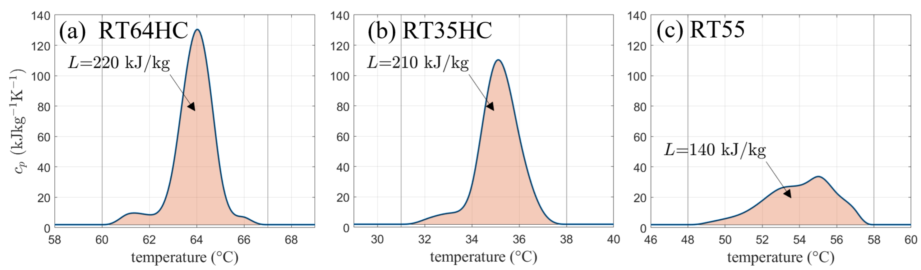
An example of a heat capacity curve of a technical grade paraffin (trade name RT64HC from Rubitherm Technologies) based on previous work by [13] with its significant peak due to the phase transition enthalphy is shown in Figure 1a.
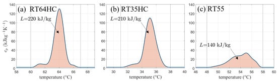
Figure 1.
Heat capacity curves including the phase change enthalpy (shaded area) for different phase change materials. (a,b) show high performance phase change materials (PCM) with 25–30% higher latent heat storage capacity compared to class PCM materials (c).
While the solidification and melting (SM) model takes into account a linear relationship of the liquid fraction between the solidus and liquidus temperatures and , the apparent heat capacity model has no clearly defined information about the liquid fraction curve. Instead, the apparent heat capacity curve contains the information about the melting temperature range and its location. Since some PCM show two peaks in heat capacity data, the model can be used for more accurate modeling of the thermophysical properties. This is especially important when focusing on technical grade PCMs with a wide melting range. However, viscosity has to be accounted for in both states. Unlike in the SM model, no automatic distinction between the two phases is included. Therefore, a temperature-dependent viscosity curve can be implemented with extremely large values in the solid state in order to mimic solid behavior [2,5].
Other approaches like a source term-based method exist as well, but shall not be explained here as this work focuses the solidification/melting model and the apparent heat capacity model.
3. Model and Materials
Two modeling approaches are compared in the following chapter, namely the enthalpy-porosity approach, which is implemented in Ansys Fluent as the solidification/melting model, and the apparent heat capacity model. Theoretical background for both models is given in Section 2.2.
The enthalpy-porosity formulation is used as the solidification and melting model (SM) in Ansys Fluent. To use it, it needs to be activated in addition to the energy equation. For material properties, a solidus and liquidus temperature are needed as input as well as density, phase transition enthalpy, heat capacity, thermal conductivity, and viscosity. The liquid fraction varies linearly over the specified temperature range for SM. Transition from the solid to the liquid phase is achieved by a user-defined parameter, the mushy-zone constant, which decreases the velocity during solidification by modification of the momentum equations.
In contrast, for applying the application of the heat capacity method (AHC), no extra model needs to be included in Ansys Fluent except from the energy equation. In the material properties panel, a temperature-dependent heat capacity curve can be implemented by different approaches like piecewise-linear, piecewise-polynomial, or any user-defined function. Since this curve contains information about phase transition range and transition enthalpy, these values do not require further specification. Phase change behavior needs to be considered by a temperature-dependent viscosity ranging from large values (solid) to very low values (liquid). Other properties like density or thermal conductivity do not have to vary between the two models. In general, both approaches strongly depend on the choice of thermophysical properties, which will be discussed in the next section.
3.1. Thermophysical Properties
In previous work, Barz et al. [13] identified phase fraction-temperature curves for commercial phase change materials in order to detect the peak shape and location of the heat capacity data. The identified phase fraction-temperature curves are shape-preserving and only need the following input: Heat capacity in the solid and liquid state, phase change enthalpy, and melting range. The model showed good agreement with experimental data from 3-layer-calorimetry and the computer code is publicly available. Further details can be found in [13]. The chosen melting ranges, liquid fraction curves, and thus the heat capacity curves in this work follow this approach.
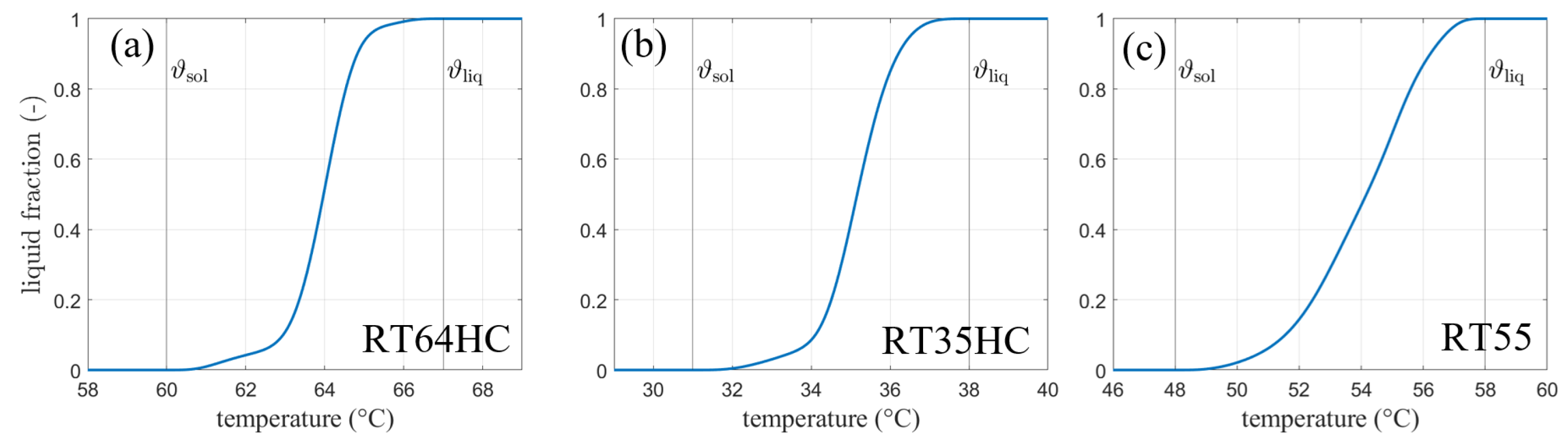
The materials with the trade names RT64HC, RT35HC, and RT55 (from Rubitherm Technologies GmbH, Berlin, Germany) are used in the presented calculations and experiments. Figure 2 shows the liquid fraction curves and the melting ranges according to Barz et al. [13].
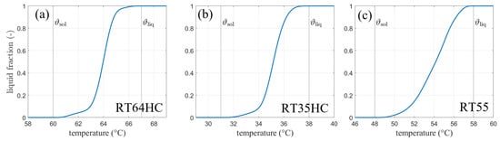
Figure 2.
Phase fraction-temperature curves for the phase change material (a) RT64HC, (b) RT35HC and (c) RT55 (all from Rubitherm technologies)—(according to [13]).
For the SM model, a linear interpolation over the given temperature ranges is used. The input for the model is summarized in Table 1. Heat capacity data were taken from the data sheets of the materials. The phase transition enthalpy was calculated according to the data sheet in the following way: For RT64HC, a total phase transition enthalpy of 250 kJ kg is provided by Rubitherm measured over a temperature range of 15 K. Given the sensible heat capacity of 2 kJ kg K, a total of 30 kJ kg can be subtracted and the final phase transition enthalpy is 220 kJ kg. Melting range data is taken from the liquid fraction curve provided by Barz et al. [13]. Please also note that the declaration of solidus and liquidus temperature might be given as and when temperature is given in Celsius and and otherwise.

Table 1.
Physical properties of phase change materials.
3.1.1. Heat Capacity
Based on this phase fraction-temperature curves, the apparent heat capacity curve can be derived by the following formula [13]:
Again, please refer to Barz et al. [13] for further information. The so obtained heat capacity curves are depicted for the materials of interest in this work.
In Figure 1, the shaded areas yield the total amount of heat stored equal to the given phase transition enthalpy L. It can be calculated from the curves by integrating the heat capacity over the melting temperature range and subtracting the product of temperature interval and sensible heat capacity or .
Since the heat capacities for the solid and liquid state are equal for all materials in this work, no further distinguishing is needed in Equation (20).
This procedure is repeated for every PCM used in this work. The curves are implemented in Ansys Fluent by a piecewise-linear function for the apparent heat capacity model. As discussed earlier, the phase transition enthalpy is given as a constant value for the enthalpy-porosity formulation used in Ansys Fluent as the SM model. In that case, only the heat capacities and phase transition enthalpies as provided in the data sheet and Table 1 is used and the heat capacity curves are not needed.
3.1.2. Dynamic Viscosity
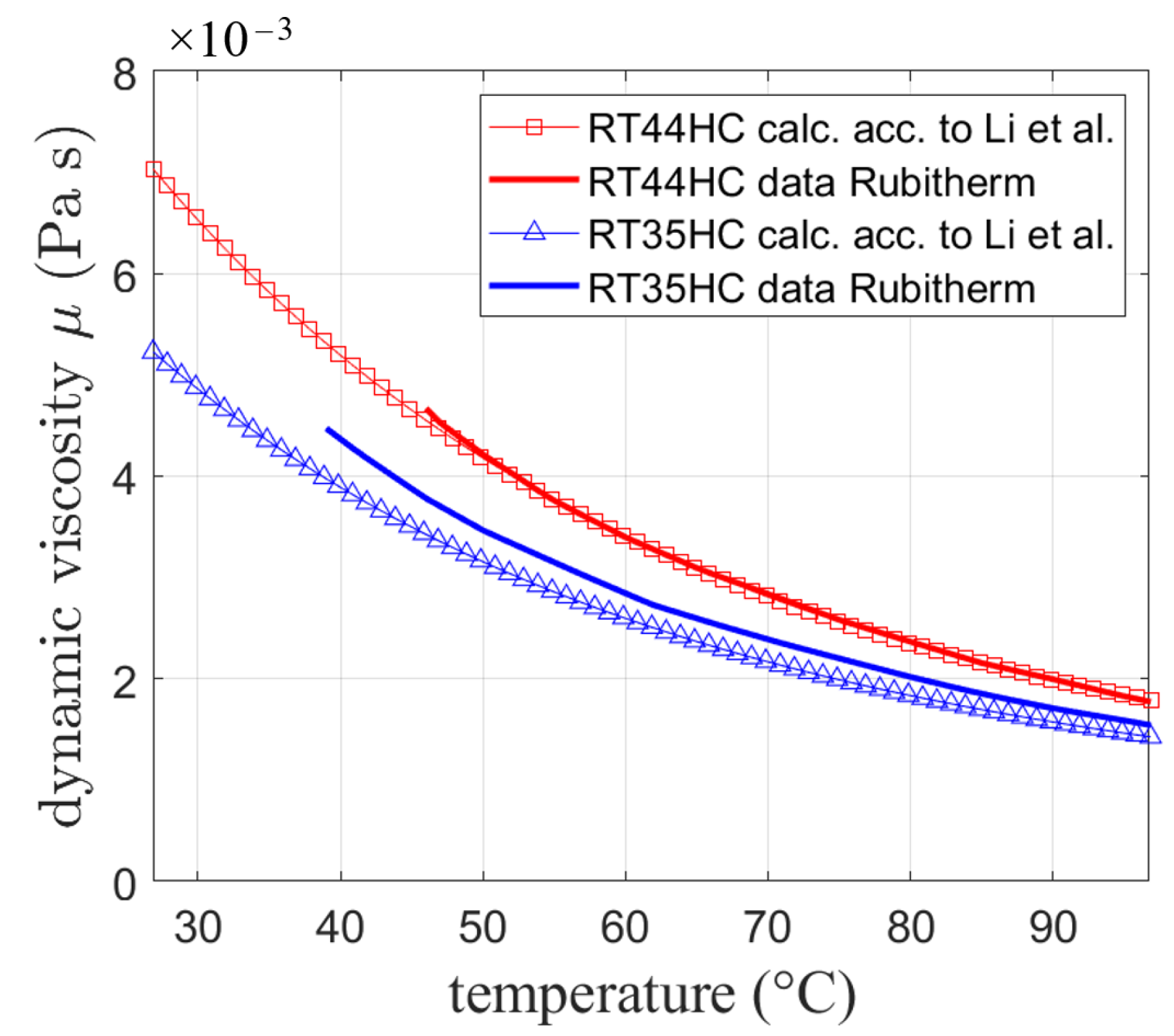
The viscosity of the materials was calculated according to Li et al. [33] with a melting temperature defined by the phase fraction curves presented in Figure 2. The melting temperatures for the phase change materials were defined as temperatures were the curves show a liquid fraction value of 0.5: (RT64HC: 64 °C (337.15 K), RT35HC: 35.1 °C (308.25 K), and RT55: 54.2 °C (327.35 K)). Li et al. [33] calculate a boiling temperature with the melting temperature as shown in Equation (21):
By means of , a viscosity can be calculated according to Equation (22):
The so obtained viscosity is compared in Figure 3 to available experimental data provided by the manufacturer for two different paraffin waxes (RT44HC and RT35HC) with different boiling temperatures calculated using the melting temperatures. Both showed good agreement between the calculations and data with a slightly higher deviation for RT35HC.

Figure 3.
Dynamic viscosity calculated by Equation (22) based on [33] compared to data from Rubitherm technologies.
While for future research work, experimental data for the respective PCMs should be collected, following the approach of Li et al. seems to be in reasonable agreement with experiments and is thus chosen for the simulation.
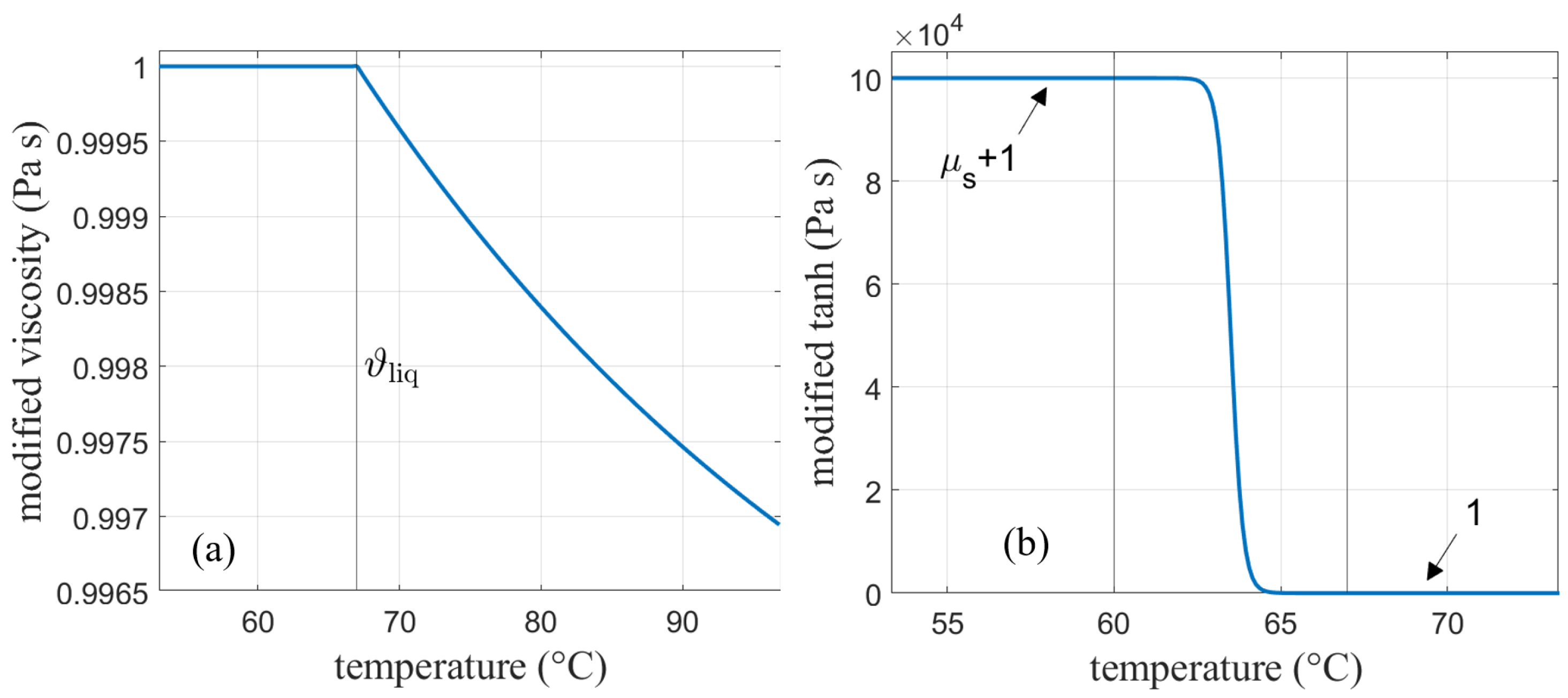
As discussed before, the SM model in Ansys Fluent mimics solidification by decreasing the velocity to zero over the melting range by means of the mushy zone constant. Therefore, no further adjustments in the viscosity need to be considered here. For AHC, the solid behavior is implemented by increasing the viscosity to very high values in the solid region [2,5]. A solid viscosity of was chosen for this work. Interpolation between the solidus and liquidus temperature was done according to a hyperbolic tangent function centered around the middle of the melting range. In order to obtain one continuous function, the tangent function and the viscosity had to be multiplied. The viscosity function calculated in Equation (22) is modified so that the part below the liquidus temperature is one and does not alter the tangent function in that region. On the other hand, the tangent function needs to be modified as well so that it does not change the viscosity curve in the liquid phase. This is done by the following modifications:
is calculated according to Equation (22) (see Figure 4a), and denotes the liquidus temperature, i.e., the end of the melting range, which is denoted by .
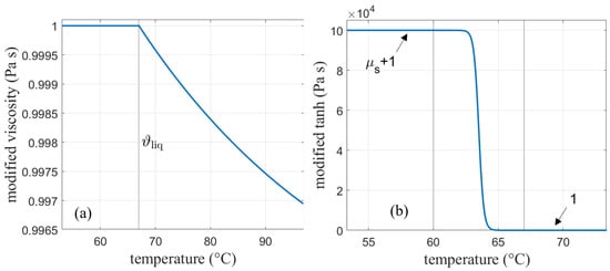
In Equation (24) (see Figure 4b), the value was calculated so that the initial deviation from the exponential function at the end of the melting range at was limited to 10 %.
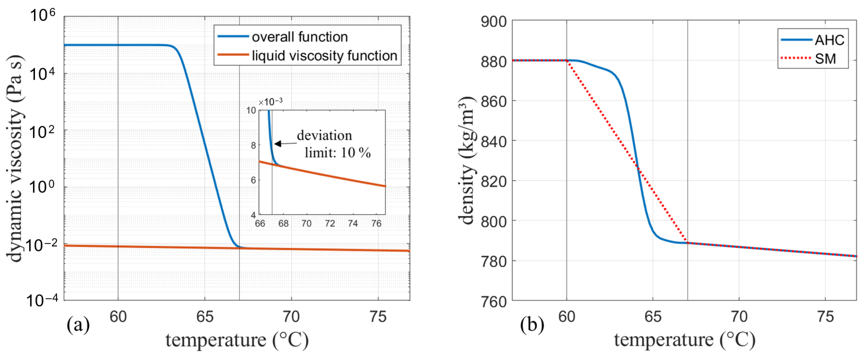
Finally, both functions are multiplied and lowered by in order to shift the function back to its initial position. The resulting function is depicted in Figure 5a together with the initially calculated viscosity function in the purely liquid region.
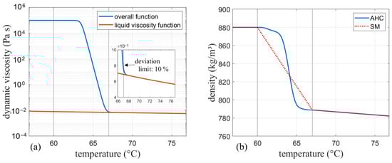
Figure 5.
(a) Final viscosity curve for the apparent heat capacity model (AHC) and liquid viscosity for comparison. (b) Density curve for AHC (var. density) and the solidification and melting (SM) model.
The finally obtained curve have been implemented in Ansys Fluent as an expression for the apparent heat capacity method. For the SM model, no artificial increase of the viscosity is needed due to the previously discussed effect of the mushy zone constant on damping of the velocities. Therefore, when the SM model is used, only the viscosity obtained by Equation (22) is implemented, which corresponds to the liquid viscosity function in Figure 5a. The presented calculation is shown for RT64HC as an example, but used for both other phase change materials in the same manner.
3.2. Density
The density in the solid region is taken as given in the data sheet (see Table 2). For the liquid phase, a linear function can be observed, e.g., [34]. Here, a negative slope of −0.68 kgm K was chosen after a comparison with literature and data provided by the manufacturer with values ranging from −0.6 to −0.76 kgm K.
Table 2.
Density parameters used for variable density and Boussinesq approach.
The density at the end of the melting range was calculated with this slope and one data point provided in the data sheet. Both models vary by the interpolation over the melting range: While SM uses a linear approach between the two temperatures, for AHC an interpolation according to the phase-fraction curve of Barz et al. [13] was implemented by a piecewise-linear interpolation:
This yields a linear transition for SM and a non-linear transition for AHC (see Figure 5b) according to the liquid fraction curves presented before.
These model approaches are compared to a simplified model using the Boussinesq approximation. For this model, the density was set to the liquid density given in Section 3.1.2 from the data sheet and the operating temperature is specified as the melting temperature from the subsection. Given the constant density, convection behavior is included in the extra term in the momentum equations while maintaining mass conservation. The validity of the Boussinesq approximation can be evaluated by comparing to 1. For the conducted cases, the expression equals a maximum of 0.0183, which is significantly lower than 1. The temperature difference ranges between 5.8 K and 21 K, which is slightly higher than the range between 10 K and 20 K suggested by [35]. Due to the fact that 2 of 3 simulation cases have temperature differences below 20 K and only one is slightly above that, the approximation is still considered plausible. Also note that there are no strict boundaries to its validity but rather a range and temperature differences above the stated range can still be accurate [35].
The thermal expansion coefficient is calculated according to with the liquid density from the data sheet and the slope of 0.68 kgm K discussed before.
Thermal Conductivity
The thermal conductivity is used for all models and all phase change materials as provided in the data sheet and accounts to 0.2 Wm K in every case presented in this work.
3.3. Model Summary
The implementation has been pursued in the commercial code ANSYS Fluent, because it is used by a wide range of authors reporting melting and solidification simulations. The presented way to describe the temperature dependence of material parameters can, however, be transferred to other Navier Stokes Solver suites (like COMSOL or the open-source environment OpenFoam) as well.
In ANSYS Fluent, both models use the PISO-scheme for the pressure-velocity coupling with a skewness and neighbor correction of 1. PISO stands for pressure-implicit with splitting of operators and is an extension of the commonly used SIMPLE (semi implicit method for pressure linked equations) algorithm. Pressure-velocity coupling being mandatory for modeling incompressible flow, SIMPLE and PISO methodologies are used throughout the different Navier Stokes solver suites.
For spatial discretization, a green-gauss node based scheme is used for the gradient, PRESTO! for the pressure and a second order upwind scheme for both the energy and momentum discretization. The PRESTO! scheme (pressure staggering option) is using a discrete continuity balance for a staggered control volume [36]. The transient formulation was chosen as a first order implicit.
In summary, the three models compared are as follows:
- Solidification/Melting (SM): Heat capacities and phase transition enthalpies are considered constant. Viscosity change over phase transition is included in the mushy zone constant of .
- Apparent heat capacity (AHC): Phase transition enthalpy is include in the apparent heat capacity curves presented in Figure 1. Viscosity change is considered by a very large viscosity in the solid phase transition and a small viscosity over phase change. Regarding density, two approaches are compared.
- (a)
- Variable density: A temperature-dependent density is used while neglecting volume change upon phase change;
- (b)
- Constant density: The Boussinesq approximation with the liquid density given in the data sheet as operating density and the melting temperature as operating temperature.
4. Results & Discussion
The solidification and melting model (SM) and the apparent heat capacity model (AHC) presented in Section 3 are compared and validated. On this basis, simulations of PCM-filled heat exchanger sample geometries can be conducted. The methodology is optimized to minimize computational cost and time. Therefore, grid independence studies including calculations using different time step sizes, have been performed.
4.1. Comparison of SM and AHC with Variable Density
In order to verify and validate the model, both models are first compared to the analytical solution of the two-phase Stefan problem. As this problem does not include gravity and thus natural convection behavior, a comparison to experimental data from measurements for RT64HC [4] and another comparison to experimental data of RT35HC from literature [2] have been performed.
4.1.1. Comparison to the Analytical Solution
For comparison of the SM and AHC models with the analytical solution of the two-phase Stefan problem, all material properties discussed in Section 3 are used. This includes a specific heat of 2000 Jkg K in both phases and a phase transition enthalpy of 220 kJ kg for SM. The melting range is given between 60 °C and 67 °C. For AHC, these information are included in the apparent heat capacity curve shown in Figure 1. The thermal conductivity for both phases and models is 0.2 Wm K. Since the comparison omits gravity and thus no variable density is needed, this is the only case where the density was set to kgm and kgm for both models. The transition, however, is done according to Equation (25) with a linear transition for SM and a transition according to the liquid fraction curve for AHC.
For comparison, a 2D-surface body with dimensions given in Figure 6a is initialized to 49 °C (322.15 K) to ensure a fully solidified state of the PCM. While the right wall was held constant at this temperature throughout the simulation, the left wall was set to a temperature of 72 °C (345.15 K). For all presented geometries, meshes with almost similar spacing in both directions have been generated. Points on all edges have been distributed uniformly using the given cell length size. Thus, the deviation from an aspect ratio of 1 is negligible. In this case, a rectangular mesh with a uniform grid spacing of 0.75 mm was used.
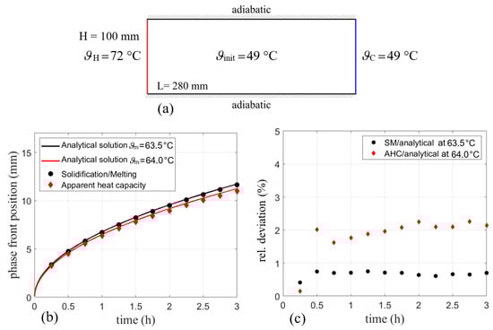
Figure 6.
(a) Simulation domain with boundary conditions for comparison with the analytical solution of the two-phase Stefan problem. (b) Phase front position for SM and AHC models compared to the analytical solutions for = 63.5 °C and 64 °C and (c) the resulting relative errors.
All walls are modeled with a no-slip condition and the walls at the top and the bottom of the enclosure were considered adiabatic. Due to the symmetry of the problem, the temperature is monitored in the middle of the shown geometry over the whole length of the enclosure.
Figure 6b shows the calculated phase front position for both models. The phase front in the analytical solution is assumed at a liquid fraction of 0.5 [5] in the discussed phase fraction curves (cf. Figure 2), which equals to a temperature of 64 °C or 337.15 K for RT64HC. For SM, the melting temperature of 63.5 °C is assumed since the transition between 60 °C (333.15 K) and 67 °C (340.15 K) is linear. The solid lines indicate the analytical solution for melting temperatures of 63.5 °C and 64 °C for comparison with SM and AHC, respectively. They were calculated according to the procedure discussed in Section 2.1. It should be noted that the Stefan problem is formulated for a well-defined melting point. As technical grade PCMs often change their phase over a temperature range, it is not clear, which temperature should be taken here as the melting temperature. As shown in Figure 6b, two options are compared. One solution is calculated for an assumption of a linear liquid fraction between the solidus and the liquidus temperature, thus resulting in a melting temperature of 63.5 °C. A second option is to define the melting temperature in terms of the liquid fraction curve shown in Figure 2. In an analogy to the chosen temperature with a linear liquid fraction, the melting temperature is defined where the phase fraction-temperature curve equals 0.5. For RT64HC, the heat capacity curve also shows a significant peak centered at this temperature of 64 °C. Another difficulty when comparing both models is the liquid fraction. While the SM model from Ansys Fluent calculates the liquid fraction in a linear manner over the melting range and provides it as output data, the AHC model only gives a temperature distribution. This can then be post-processed and used for calculation of the liquid fraction.
On the one hand, liquid fraction results from the SM model are in good agreement with the analytical solution for a melting temperature of 63.5 °C. This was expected, as Ansys Fluent uses the linear relationship between solidus end liquidus temperature. On the other hand, the liquid fraction obtained by the phase fraction curve for AHC is in good agreement with the analytical solution of 64 °C. The relative deviation of the numerical solution to its analytical solution is depicted in Figure 6c, which refers to the deviation of the simulated points with regards to their respective analytical solution. The SM model used in Ansys Fluent has small relative deviations (<1%) compared to the analytical solution while for AHC the deviations are about 2%. The slightly higher deviation for AHC might result from the asymmetric heat capacity curve, which has two side peaks resulting in a non-linear phase change, cf. Figure 1. This might be more difficult to characterize by a single melting temperature than a purely linear phase change as applied in SM. The deviations for both models in general may result from inaccuracy of the analytical solution for melting ranges since the Stefan problem is formulated for a clearly defined melting temperature, so no exact alignment is to be expected. Being given the melting range of 7 K, none of the analytical solutions can be declared as the correct one. Therefore, the comparison only shows the verification of the respective method. With a significant peak of the heat capacity data at 64 °C, AHC might match a more physical explanation of the problem and is thus preferred here.
4.1.2. Comparison to Experimental Data with Gravity and Natural Convection
Another important factor when comparing both models is the natural convection behavior. Modeling is achieved through a temperature-dependency of the density in the liquid phase. First, both models are compared to experimental results conducted with RT64HC as PCM [4]. Second, the model is applied to RT35HC in order to compare the resulting phase front to literature data [2].
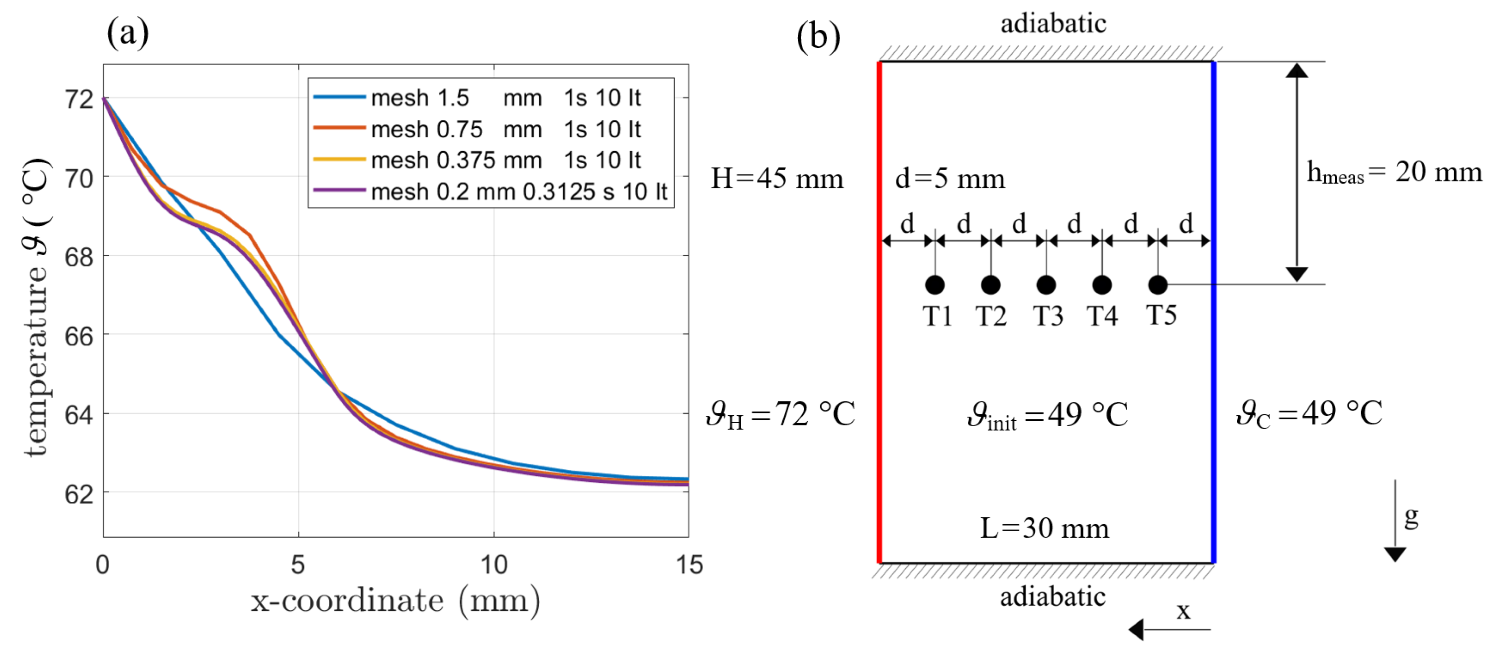
First, a mesh refinement study was conducted in order to find the required cell size. For this purpose, a cube with an edge length of 15 mm was heated to 72 °C (345.15 K). The initialization temperature was set to 49 °C (322.15 K) and all other walls were considered adiabatic. Gravity was included and the AHC model was used with variable density. The temperature was monitored over a line placed in the middle of the heated wall extending to the opposite wall.
Simulations with different time steps have been performed and a time step of 1 s has been found to provide good results (see Figure 7a) for the comparison of 0.3125 s to 1 s). A total of 10 iterations for each time step have been always used for the simulation. The stop condition in the transient runs therefore was fixed to 10 iterations per timestep, which was enough to establish the necessary drop and relaxation in residua. The choice of 1 s and 10 iterations led to good time efficiency while keeping accuracy. The simulations with different grid spacing favored a cell size of 0.375 mm, since no significant change occured when further refining the mesh.
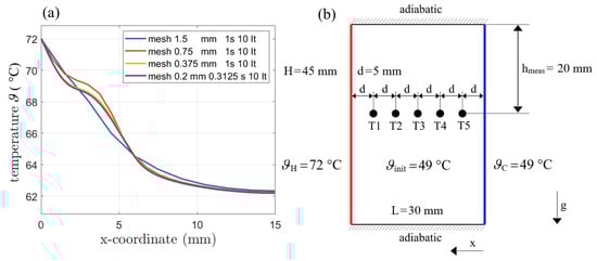
Figure 7.
(a) Mesh refinement for AHC (var. density) for different mesh sizes. Time steps and iterations did not alter the results. (b) Simulation domain including the boundary conditions and positions of the temperature sensors.The phase front is tracked at the top of the enclosure.
The time step size and the iteration count were found to have no influence on the resulting temperature distributions. Therefore, the following simulations are performed with a mesh size of 0.375 mm and a time step of 1 s.
4.1.3. Comparison with RT64HC Data from AIT measurements
In [4], the melting process of PCM was investigated by optical tracking of the phase front in a rectangular enclosure from above and extracting the phase front with an edge detection technique. With tempered walls at the sides, the moving of the phase front was observed through an acrylitic glass plane (polymethoylmetacrylat, PMMA) from above. In the PCM, PT100 temperature sensors were placed every 5 mm in a depth of 20 mm. The problem is considered symmetrical, therefore a 2D simulation is conducted. Boundary and initial conditions are given in Figure 7b. A rectangular mesh with a uniform grid size of 0.375 mm is used as discussed within the mesh refinement section. The temperature for the phase front calculation is monitored at the top of the enclosure to reconstruct the optical measurement from above and temperature sensors are simulated by monitoring the temperature in the same height of the enclosure as temperature sensors have been placed.
Material properties for both simulation methods, SM and AHC, were chosen according to Section 3.
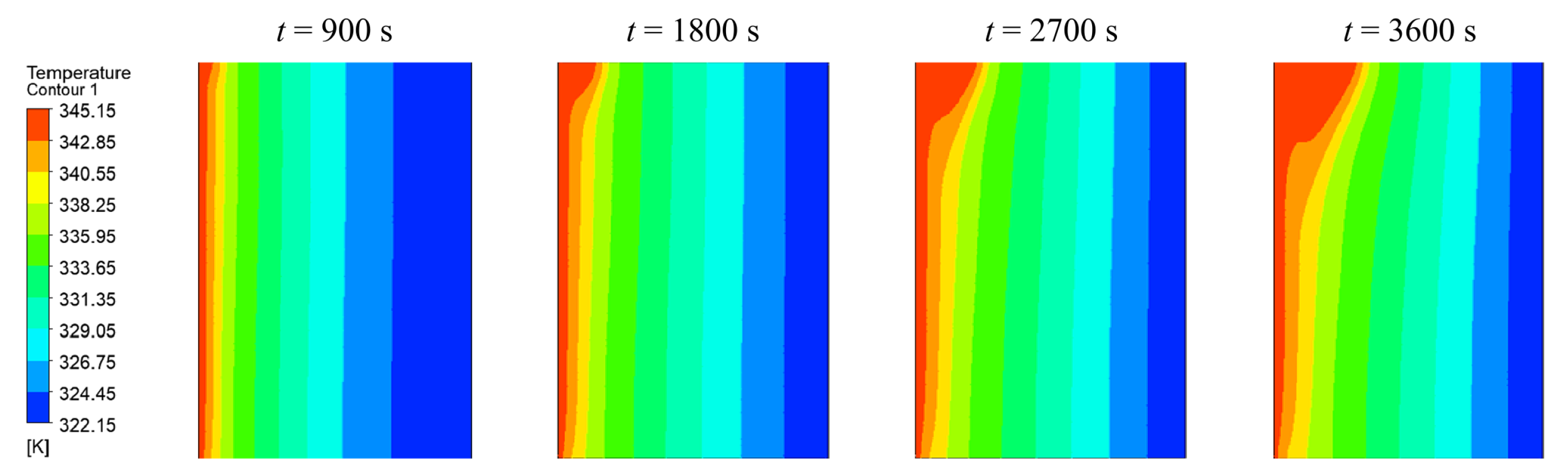
Figure 8 shows the temperature distributions obtained with the AHC (variable density) model after 900 s, 1800 s, 2700 s, and 3600 s from left to right. In the first subfigure, the PCM begins to melt from the heated side of the wall uniformly. After 1800 s, the liquid phase starts to bulge in the upper part of the enclosure, which is than further intensified over time until a steady-state is reached.
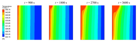
Figure 8.
Temperature distribution using AHC model after 900 s, 1800 s, 2700 s, and 3600 s.
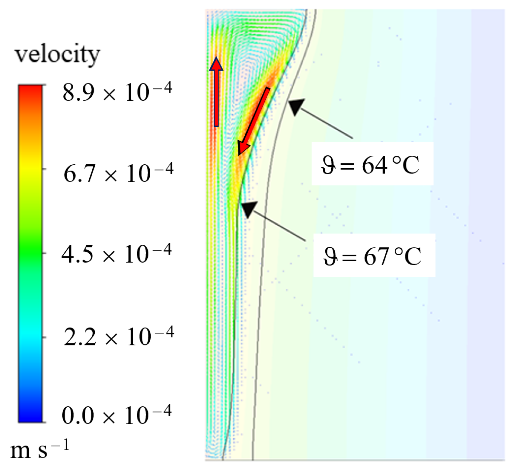
This behavior is induced by natural convection, which is well known in literature [2,5,6,29,37,38,39]. Due to the temperature dependent density, liquid PCM rises at the hot wall due to its smaller density and descending at the colder phase front [38]. A circular fluid current in the liquid phase develops. This is also illustrated in Figure 9, where the velocity magnitudes are indicated in the temperature profile of 3600 s.
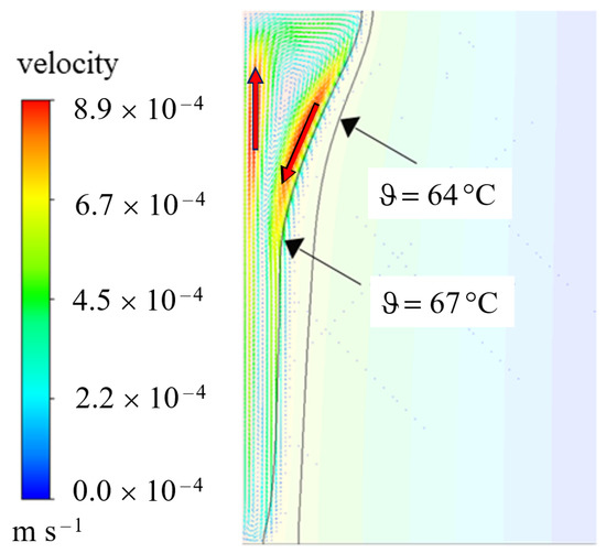
Figure 9.
Velocity profile at 3600 s for the AHC model with a bulged shape of phase front due to natural convection (compare also to Figure 8).
As marked by the red arrows, the velocity at the walls of the liquid phase is the highest with an upwards movement at the heated wall and a downwards movement at the liquid phase front. For comparison, both the melting temperature and the liquidus temperature are added as isolines. According to and , the Rayleigh number can be calculated for this example by the following assumptions:
- ;
- ;
- .
Convection is only assumed in the purely liquid region, hence the temperature difference is set to the difference between the hot wall and the liquidus temperature. The thermal expansion coefficient is set to the value discussed in Section 3. The Rayleigh number would exceed the limit discussed in [40] of approx. 1000 as the critical Rayleigh number at a phase front position of approximately 3 mm. In the presented example for AHC (var. density), the phase front reaches this value after 1080 s (18 min), cf. Figure 10. As this is shortly after the first image at 900 s, this might explain the transition to the bulged behavior between 900 s and 1800 s since conditions in the liquid phase reached a thermally unstable state [40]. Below the critical Rayleigh number and thus before the stated time, natural convection is weak and heat is transferred primarily by conduction [40].
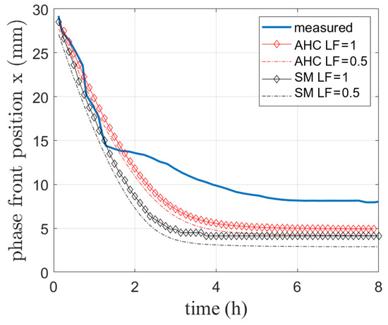
Figure 10.
Simulated and visually measured phase front position during melting of RT64HC conducted in [4].
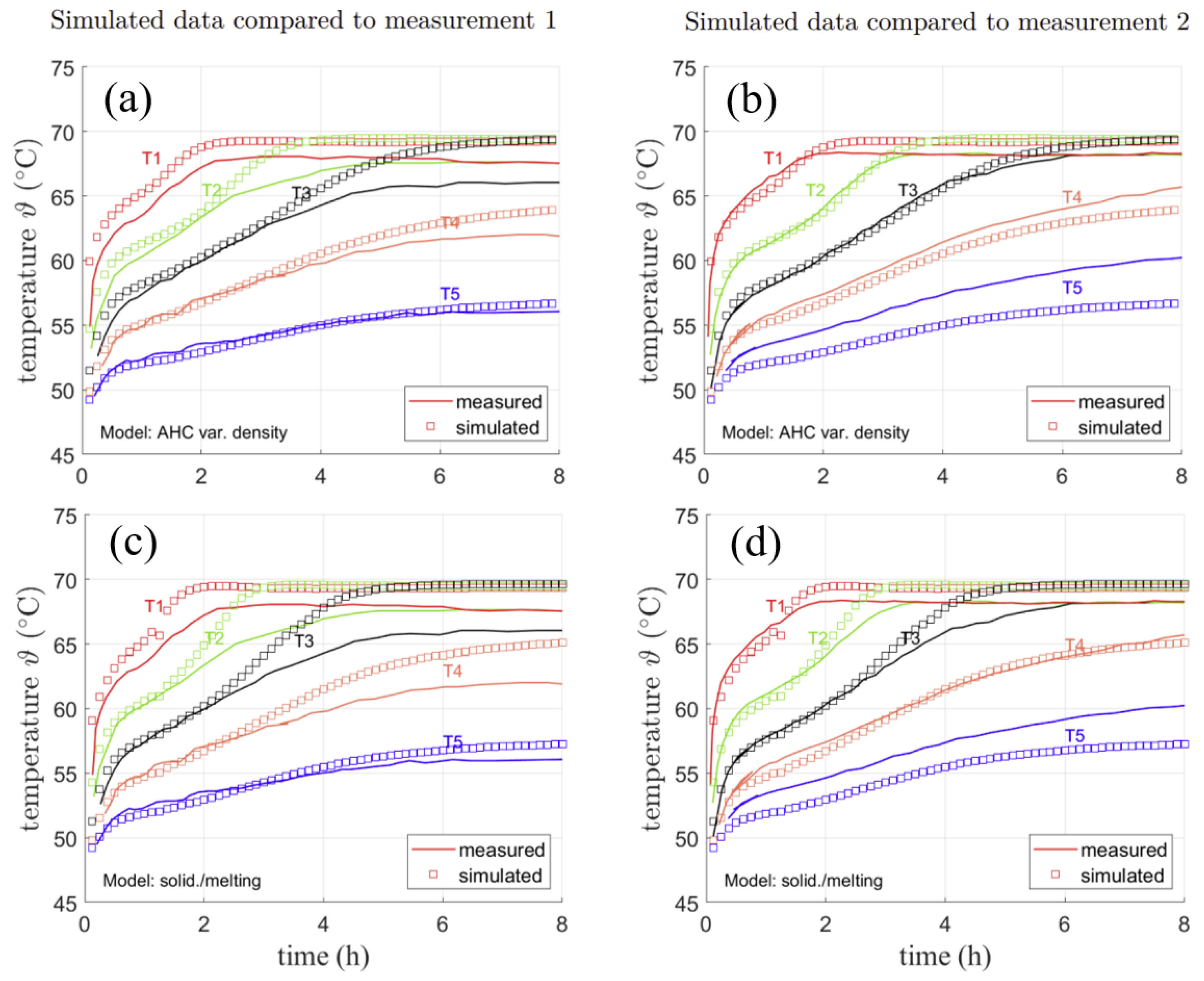
Figure 11a,b shows the comparison of the AHC model to experimental data obtained by solid lines. From top to bottom, they represent the sensors from the hot wall to the cold wall with a distance of 5 mm each. Therefore, the first sensor in a distance of 5 mm to the hot fin is represented by the upmost curve, the second sensor in a distance of 5 mm to the first is shown by the second upmost curve and so on. The measurement has been conducted twice with slightly different results. For the sake of an objective comparison to the data and its evaluation regarding measurement inaccuracy, both measurements are shown in Figure 11a shows data obtained in a first measurement and Figure 11b data obtained in a second measurement. Simulated temperature points are shown as markers in both measurements. Please note that simulated data is the same in both figures. Here, the temperature at the sensor positions from AHC (variable density) from the previously shown temperature distributions are shown.
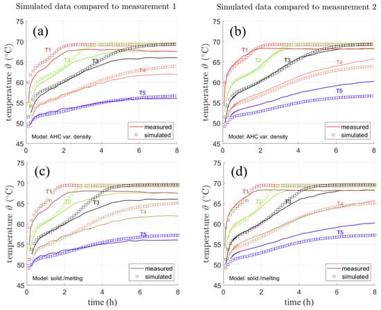
Figure 11.
Measured and simulated temperatures for two repeated simulations conducted in [4] for AHC with variable density (a,b) and SM (c,d).
In Figure 11a, the temperature measured at the nearest two sensors to the cold fin (T4 and T5) can be reproduced by simulation results with a deviation of about 2 K. They stay in solid PCM throughout the whole measurement, indicating that the position of the sensors is fixed. The third temperature sensor T3 is in very good agreement with the measured temperature until approx. 4 h. Then shown by the temperature simulated and measured at this point, the phase front reaches the sensor. As the monitored point is reached by the liquid phase, its temperature increases towards a uniform temperature of approx. 69 °C over the further simulation. For the first two temperature sensors T1 and T2, a deviation of max. 2.6 K from the measurement data is observed in Figure 11a. They reach the same temperature after approx. 3 h in Figure 11a,b, which clearly indicates a uniform temperature distribution due to convection in the liquid part of the domain. As the liquid phase reaches them at an earlier stage, their temperature quickly reaches the maximum temperature. In Figure 11b, the measurement was carried out again. While the lower temperature curves for T4 and T5 show stronger deviations of about max. 4 K, the sensors in the liquid state (T1-3) can be well reproduced (≈1 K deviation) by simulation results. Both the curve shapes and the time when the upper two temperature curves reach the same value match the simulated results. It should be noted that the measurement is subject to uncertainties. This is also shown by the fact that the same measurement was conducted twice with locally different temperature results. This might result from positioning of the sensors in the initial state as well as shifting of their exact position during phase change. The used sensors had a diameter of about 2 mm. Hence, small deviation in positioning is very likely. Furthermore, ref. [4] recorded problems with tightness of the PCM enclosure. However, the results can still be used for qualitative comparison of the model. The same simulation was also conducted for the SM model with a mushy zone constant of . As can be seen in Figure 11c, the SM model yields similar temperature curves as the AHC model, but with larger deviations from the measured curves about max. 4–5 K for T3 in Figure 11c and about 3 K for T5 in Figure 11d. The mushy zone constant, however, is rather high with . Any smaller mushy zone constant resulted in an nonphysically fast melting of the PCM or solver divergence. The high constant might be needed due to the wide melting range over 7 K, which was chosen in accordance to the AHC model. However, as the heat capacity curve in the beginning does not show a significant rise, it might also be reasonable to consider a smaller melting range and thus a smaller region with lowered viscosity. This might lead to similar results, but with a smaller mushy zone constant.
In Figure 10, the measured phase front position is compared to the results of both the SM and AHC model. The phase front positions of the completely melted state (LF = 1) as well as when phase change has reached a LF of 0.5 as discussed for the analytical solution are shown.
Both models reproduce the initial melting process up to approx. 1.5 h. The steady state reached at the end differs from the experiment by 3 mm for AHC and 3.8 mm for SM for the curves at LF = 1. This deviation might result from difficulties detecting the exact position of the phase front as well as e.g., heat losses to the environment. Due to the PMMA at the top, this wall can not be considered adiabatic. This heat loss can not be completely avoided in the experiment to allow for optical phase front observation. During solidification experiments, it was also observed that the phase front established faster around the sensors, which are building a conductive bridge to the outer environment. Therefore, a heat loss through the sensors might also occur. As this lost energy is not available for the melting process, the phase front moves less forward than the simulated one.
In addition, the previously mentioned uncertainty for sensor placing and their diameter of 2 mm might add deviations here. However, the phase front position for the completely melted state is about 1 mm above the curve for LF = 0.5. It is very likely that visual tracking only allows distinguishing between the solid and the liquid phase without a visible mushy zone. This will also be discussed in the next subsection.
In summary, given the agreement with only small deviations in temperature (about 3 K) and phase front position (about 3 mm), it is assumed that the model can be used to predict phase change in a reasonable way even when natural convection behavior is included. For further validation, a comparison to literature data is drawn for an additional different PCM.
4.1.4. Comparison with RT35HC Data from Literature
The methodology for PCM modeling was initially developed for RT64HC and has been transferred to other PCMs. To validate the model for different PCMs, a comparison to literature data of [2] is drawn. Their work also includes visual tracking of the phase front. While [4] monitored the phase front from above, they tracked the phase front movement from a side-view revealing the shape of the phase front. A 2D rectangular enclosure was modeled, 40 mm × 40 mm and a mesh size of 0.375 mm as well. The left wall of the enclosure was heated to 315.5 K and the right wall to 303.15 K. Top and bottom wall were considered adiabatic.
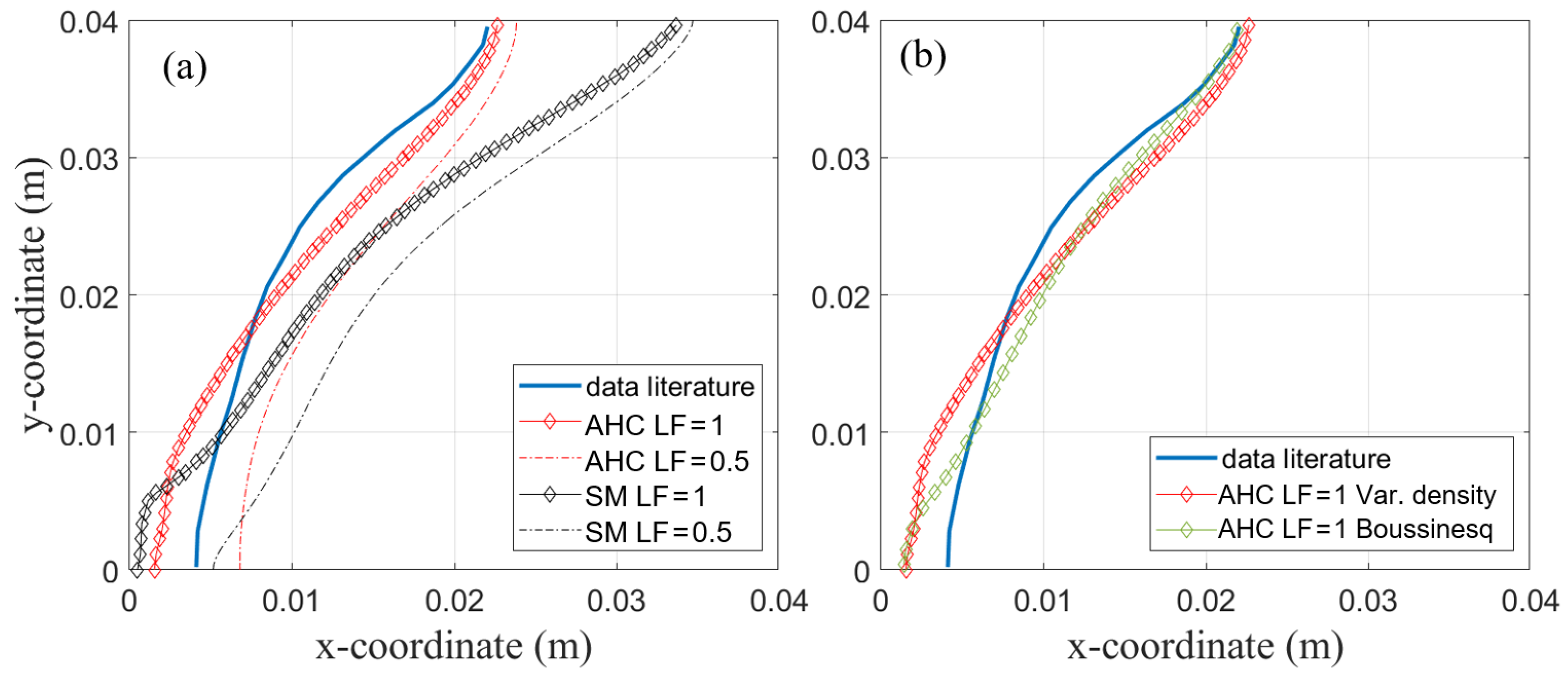
Figure 12a shows the experimentally measured phase front position obtained by [2] compared to the simulated position by the SM and AHC model. The visually tracked phase front was compared to data at a fully melted state, i.e., liquid fraction equals one, and at a liquid fraction of 0.5.
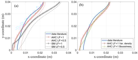
Figure 12.
(a) Phase front visually measured after t = 2 h provided in [2]. (b) Comparison of AHC model with variable density and Boussinesq approximation for data from [2].
The shape of the phase front is modeled very accurately with AHC, especially in the upper part of the enclosure. In the lower part, deviation is a little higher with about 2 mm. This might be due to material properties, e.g., a constant thermal conductivity assumed in the simulation. Furthermore, as discussed in the previous chapter, different measurement uncertainties like heat loss to the environment might be a possible explanation. Better agreement was shown with the completely melted phase front. Though not being discussed in their paper, it is very likely that the fluid and solid phase can be distinguished visually without notice of the mushy zone as mentioned before. Thus comparing the results to the phase front of the completely melted state seems to be the better option. The deviation from the measured phase front is higher for the SM model with a deviation from the measured curve at the top of the enclosure of about 10 mm. Interestingly, for the comparison in the previous section, AHC and SM resulted in nearly the same phase front position (about 2 mm deviation from one another) viewed from above and only differed in the temperature in the domain. Based on these previous results (see Figure 10), one might expect the phase front at the top of the enclosure at y = 40 mm to be more similar. In Figure 12a, this position differs by about 10 mm. Maybe for SM, the mushy zone constant would need further adjustment. In contrast, the AHC model seems to model the phase change more universally without the need to adjust parameters and is thus preferred here.
Comparison to both the data from the new experiment as well as literature data strongly suggests a good prediction of the phase front movement and the temperature with the AHC model. The SM model in Ansys Fluent seems to be more difficult to apply to different cases. The mushy zone constant acts as an undefined parameter mostly used to fit experimental data [5]. Since the presented AHC models does not need such a parameter and showed good agreement for different applications, it is chosen for further simulations. While previous simulations were performed with the variable-density approach, the next subsection focuses on the AHC method only and discusses the difference between applying a variable density and a Boussinesq approach for natural convection.
4.1.5. Comparison of AHC with Variable Density and Boussinesq Approximation
While the presented results suggest a good agreement between simulation and experiments, volume expansion is neglected with variable density and a fixed volume. Therefore, mass decreases with temperature over the course of the melting process. Hence, a second method for AHC was used in order to investigate the magnitude of error regarding temperature and heat flow. For RT64HC, the Boussinesq approximation is used with a fixed density of 780 kgm and an operating temperature of 64 °C (337.15 K). The solution methods used stayed the same as described in the previous section.
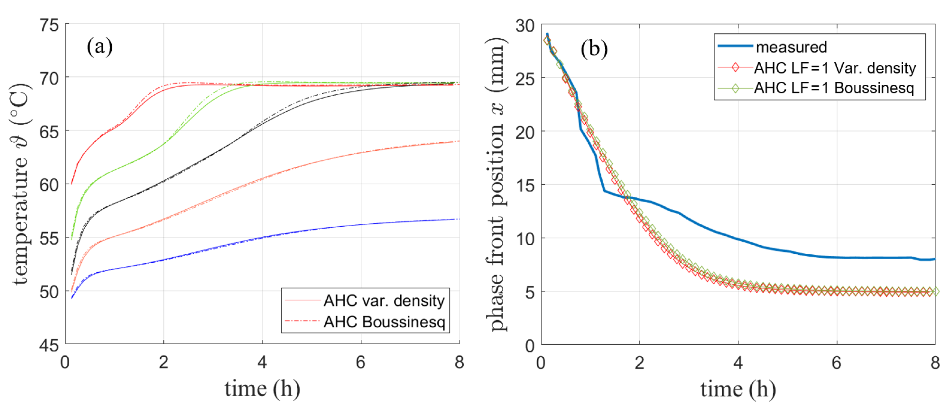
Figure 13 shows the comparison of the AHC method for the variable density approach and the Boussinesq approximation regarding the simulated temperature curves (a) and the phase front position (b). The comparison refers to the data presented in Section 4.1.2.
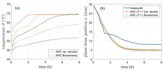
Figure 13.
Comparison of AHC model for variable density and Boussinesq approximation regarding (a) temperature and (b) phase front position.
The comparison between the variable density approach and the Boussinesq approach is also performed for the validation simulation with literature data presented in Section 4.1.2. The resulting phase front after 2 h shown in Figure 12b still matches the results presented by [2] well. The shape of the phase front is only slightly different for both models.
The results suggest that for the purpose of monitoring the temperature neglecting the volume expansion by using a variable density with a fixed simulation volume has only a minor effect on the results. However, mass and thus energy conservation are violated with variable density and therefore the Boussinesq approximation has been chosen in the further course of this work.
Adding an air phase to the domain in order to allow for volume expansion and track the PCM by a volume of fluid-approach in Ansys Fluent would have been an alternative approach. However, due to the obvious fact that applying the Boussinesq approximation is less complex while still providing a good agreement to experimental data, the Boussinesq approximation is the preferred approach.
4.2. Validation of the PCM Model with Fins
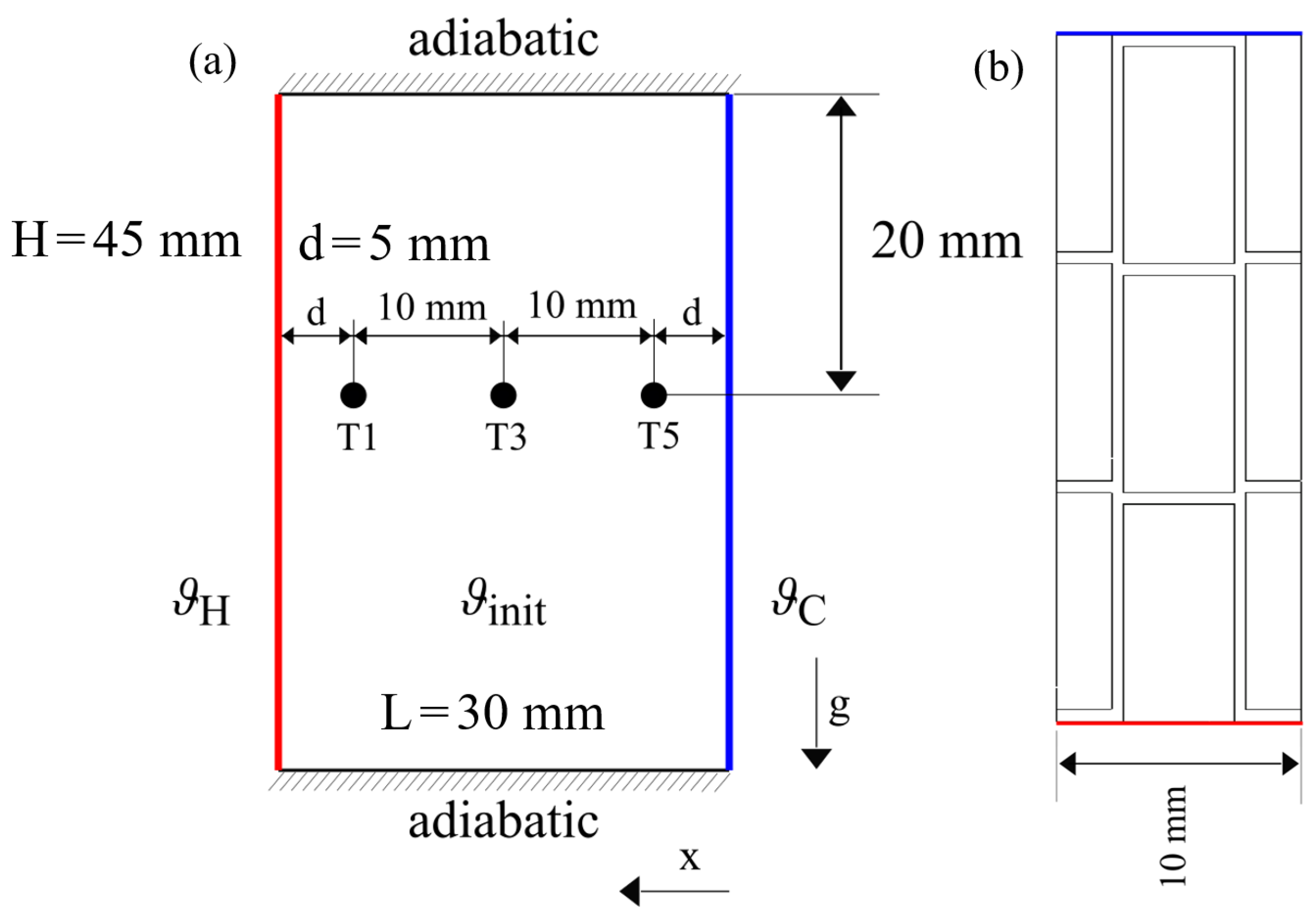
Since the model has been validated so far using pure PCM, the integration of metal fins and its impact on the model needs to be tested and verified. The geometry and fin structure is presented in Figure 14 as described in [4]. Again the PCM material RT64HC is used. The simulation was conducted according to the scheme presented in Figure 7b. The introduction of fins needs a change from 2D to 3D simulation. The mesh has been created using hexahedral cells with a uniform grid size of 0.5 mm as this was the approximated fin thickness.
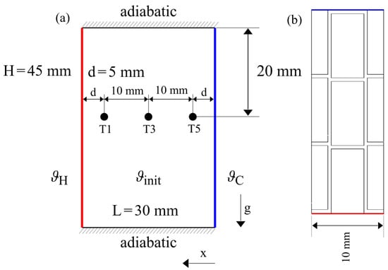
Figure 14.
Simulation domain with boundary conditions from (a) sideview and (b) topview. The fins have been omitted in the side view (a) to increase readability.
Due to the fin geometry, sensors T2 and T4 are left out, but all other measurement positions remain. Temperature is monitored in a depth of 20 mm from the top while the melting front is calculated from the temperature of the top of the enclosure to replicate the visual tracking from above.
Both the melting and solidification processes were simulated using the AHC method with Boussinesq approximation.
4.2.1. Melting
For the melting process, boundary and initial conditions are chosen as follows:
- heating from 34 °C to 70 °C (hot fin) in 12 min;
- constant temperature of 34 °C (cold fin);
- Initial temperature 34 °C.
The simulation was repeated with a uniform grid size of 0.25 mm in order to avoid mesh refinement errors, but no difference was observed with a finer mesh.
As depicted in Figure 7a, the hot and cold fin were given as boundary conditions according to the experimental setup, while the temperature of sensors T1, T3, and T5 was monitored at three points across the domain.
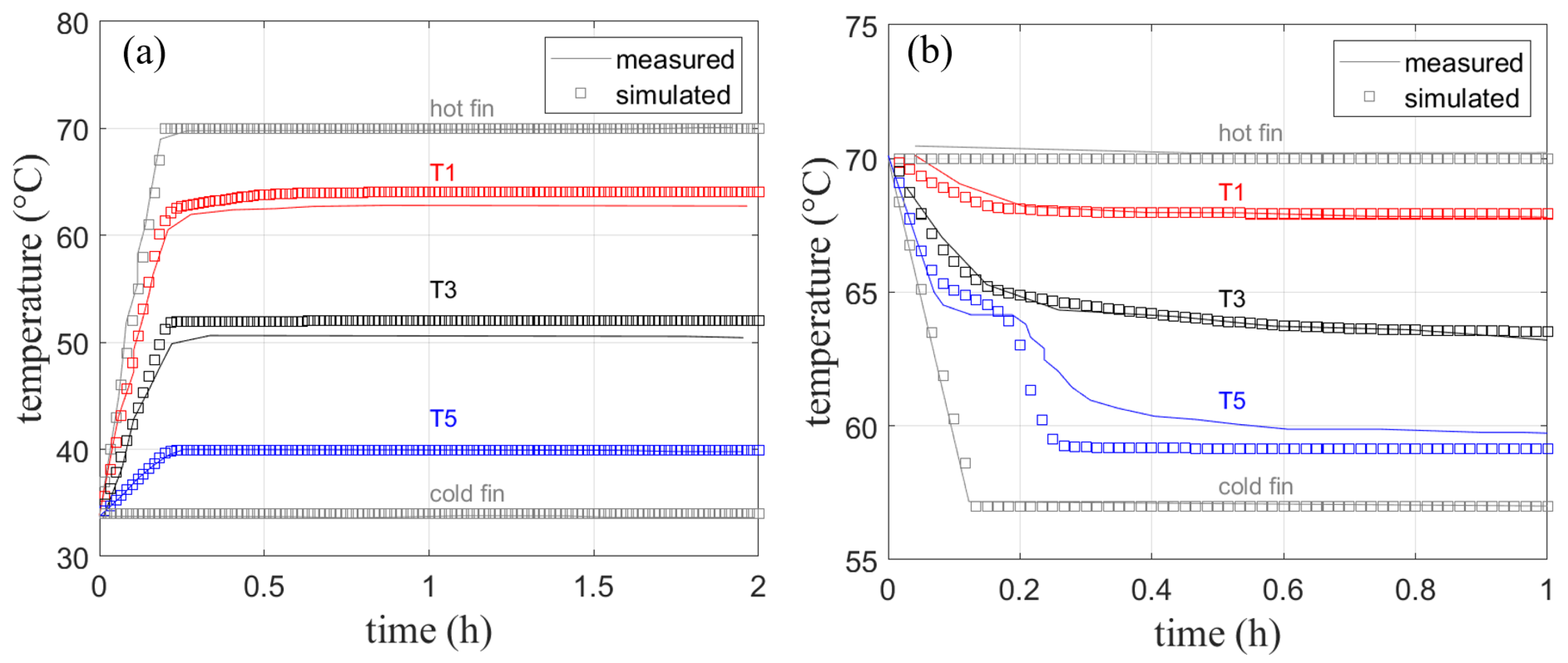
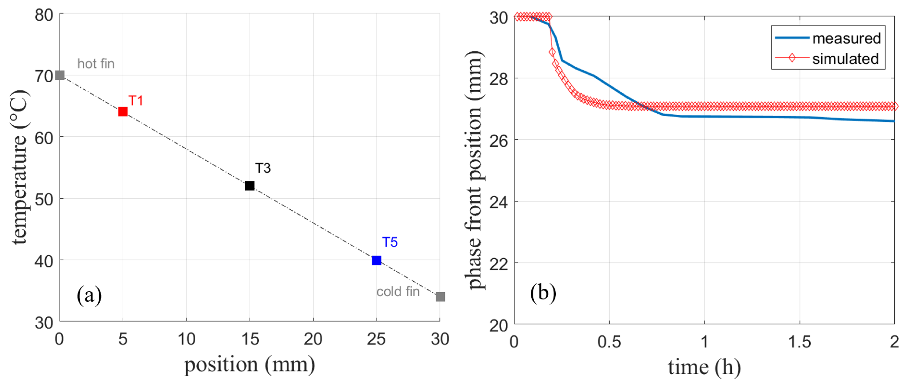
The simulated temperature in Figure 15a shows only deviations from the measured temperature of about 1 K. This deviation might result from measurement uncertainties, heat loss to the environment, or slight differences in the fin thickness used in the experiment. The heat loss to the top is, however, much less of a concern compared to the experiments without fins presented earlier, as fin experiments run much faster. Given the distance between the sensors, a linear temperature profile can be observed due to pure heat conduction shown in Figure 16a. As no significant velocities are observed in the finned geometry, further simulations are performed with the assumption of a negligible natural convection when fins of this size are used.
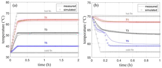
Figure 15.
Measured [4] and simulated temperature curves with fins for (a) melting and (b) solidification. Note, that for melting (a), only sensor T1 is placed within the melting zone.

Figure 16.
(a) Temperatures of the sensors at t = 2 h reveal a linear temperature profile. (b) Simulated phase front position compared to the measured position from [4].
Figure 16b shows the measured and simulated phase front position. The position when the experiment has reached a stationary state shows a constant offset. The curvature after the initial phase front movement is not well reproduced. As mentioned in Section 4.1.2 for the same experiment without fins, the detection of the phase front position using a top mounted camera is prone to uncertainties, especially during the dynamic phase change.
4.2.2. Solidification
The larger scope of the work presented here lies on the charging of the PCM-filled heat exchanger, which only includes melting of the phase change material. However, in a real application discharging the heat exchanger would result in solidification of the PCM. Therefore, a solidification experiment has been conducted and simulated in order to verify the models ability to simulate both directions of phase change. The boundary and initial conditions for this experiment were chosen as follows:
- 70 °C;
- 70 °C to 57 °C in 8 min;
- Initial temperature 70 °C.
Simulated and measured data shown in Figure 15b are in good agreement with each other especially for T1 and T3. Their temperature curves are reproduced without visible deviation from the measured temperatures. Only the last temperature sensor T5 shows a larger deviation from the measured data as the material there clearly undergoes solidification. A temperature plateau at the melting temperature of 64 °C is visible in both measured and simulated data. The final temperature after 1 h shows a deviation of approx. 1 K. Taking into account the previously discussed measurement uncertainties, the agreement with measured data is very good. It should be noted that the solidification and melting processes do not follow the exact phase fraction-temperature curves, therefore solidification would result in a slightly different heat capacity curve [3] for the cooling process, which was not implemented for this comparison.
5. Conclusions
Both the SM and AHC model approach have been compared to the analytical result of the two-phase Stephan problem. Both models showed only small deviations (<2%), a slightly higher deviation for AHC being attributed to the asymmetrical heat capacity curve resulting in a nonlinear phase change, which is not included in the two-phase Stephan problem.
To utilize the AHC approach to its full potential, it is important to correctly implement the temperature dependence of the material parameters. This is especially true for the viscosity, where a continuously differentiable function has been implemented. A piecewise linear description is enough for the heat capacity and density, whereas conductivity can be also considered constant.
For the comparison with experimental data, temperature dependency in the density was introduced. This allows for the inclusion of gravity effects and thus the establishment of natural convection. Temperature distributions driven by the rise of liquid PCM at hot walls followed by descending behavior at the colder phase front could be established. The shape of the phase front is modeled very accurately with AHC, especially in the upper part of the enclosure. It can be concluded that the phase prediction using the SM and AHC approach still holds, when natural convection behavior is included. For both the experimental data sets with RT35HC and RT64HC, the AHC approach allows for good prediction of the phase front movement and the temperature distribution. The SM model seems to be more difficult to apply to different cases as the mushy zone constant is mostly used to fit experimental data. For AHC, however, in the solid region a viscosity has to be defined using an artificially large value. The influence of this value has been found to be more acceptable. It is very important to introduce a continuously differentiable formulation of the temperature dependence of the viscosity for AHC to provide stable results. In this paper, this was achieved using a tanh-trigonometric function. Since AHC does not need the mushy zone parameter and proved to provide valid results for different data sets, it is recommended by the authors.
The results show that the variable density approach has enough accuracy, when the main interest lies in monitoring temperatures. The variable density approach with fixed volumes leads to a violation of the conservation of mass and energy within the modeled volume. To avoid high computational costs and long calculation times, the AHC has been modified by introducing the Boussinesq approximation, which is a less complex concept compared to switching to a multiphase volume of fluid approach, including an additional air volume above the PCM. The Boussinesq approach general is valid only for small temperature ranges depending on the given isothermal expansion coefficient. Good agreement was achieved using the Boussinesq approximation in an exemplary fin geometry comparing the temperature distribution of the simulations to experimental data.
In AHC, the temperature dependent latent heat capacity curve of the PCM material (extracted from measurements) is implemented. If a comparative SM calculation uses a latent heat capacity exactly matching the integral below this curve, final temperatures using SM and AHC will match. If the focus is set to part load conditions, where the melting or solidification process is in progress, however only AHC will be able to predict correct results for the temperature and phase front. The use of AHC in part load conditions is all the more important as the greater the deviation of the latent heat capacity from its average value.
As a concluding remark, the authors favor the use of the AHC modeling approach with the Boussinesq approximation provided that the heat capacity curve is represented appropriately to on the one hand to avoid the uncertainties in selecting the mushy zone constant and on the other hand, provide fast and reliable simulation results without having to use volume-of-fluid multi-phase modeling approaches.
Author Contributions
Conceptualization, C.R., J.E., and S.B.; methodology, S.B., C.R., and J.E.; software, S.B.; validation, S.B., P.M., J.E., and C.R.; formal analysis, S.B. and P.M.; investigation, S.B. and P.M.; resources, J.E. and C.R.; data curation, P.M. and S.B.; writing—original draft preparation, S.B.; writing—review and editing, C.R. and J.E.; visualization, S.B.; supervision, J.E., C.R.; project administration, J.E.; funding acquisition, J.E. All authors have read and agreed to the published version of the manuscript.
Funding
This research was funded by the Austrian Research Promotion Agency (FFG) under grant no. 879449 (program line ‘Stadt der Zukunft’, project ‘CHALLENGE’).
Institutional Review Board Statement
Not applicable.
Informed Consent Statement
Not applicable.
Data Availability Statement
Not applicable.
Conflicts of Interest
The authors declare no conflict of interest. The funders had no role in the design of the study; in the collection, analyses, or interpretation of data; in the writing of the manuscript, or in the decision to publish the results.
Abbreviations
In the following, letters, indices, and abbreviations used in this work are listed. Please note that indices and symbols that only appear once or are self-explanatory are omitted here.
| Latin letters | Unit | |
| a | Temperature diffusivity | m s |
| C | Mushy zone constant | kgs m |
| Specific heat capacity | Jkg K | |
| Liquid fraction | - | |
| Grashof number | - | |
| Enthalpy (specific) | J (Jkg) | |
| L | Latent heat | Jkg |
| Characteristic length | m | |
| m | Mass | kg |
| Rayleigh number | - | |
| Reynolds number | - | |
| Stefan number | - | |
| T | Temperature | K |
| x | Vapor quality | - |
| X | Phase front position | m |
| Greek letters | Unit | |
| Heat transfer coefficient | Wm K | |
| Thermal expansion coefficient | K | |
| Temperature | ||
| Thermal conductivity | Wm K | |
| Dynamic viscosity | kgm s | |
| Kinematic viscosity | m s | |
| Density | kgm | |
| Sub-scripts | ||
| c | cold | |
| g | gaseous | |
| H | hot | |
| in | inlet | |
| init | initial | |
| L | low | |
| l | liquid | |
| liq | liquidus | |
| m | melting | |
| m | mass | |
| o | operating | |
| s | solid | |
| sol | solidus | |
| v | volume | |
| w | wall | |
| Abbreviations | ||
| AHC | Apparent heat capacity model | |
| DSC | Differential scanning calorimetry | |
| LF | Liquid fraction | |
| PCM | Phase change material | |
| SM | Solidification and melting model |
References
- Iten, M.; Liu, S.; Shukla, A. Experimental validation of an air-PCM storage unit comparing the effective heat capacity and enthalpy methods through CFD simulations. Energy 2018, 155, 495–503. [Google Scholar] [CrossRef]
- Kasibhatla, R.R.; König-Haagen, A.; Rösler, F.; Brüggemann, D. Numerical modelling of melting and settling of an encapsulated PCM using variable viscosity. Heat Mass Transf. 2017, 53, 1735–1744. [Google Scholar] [CrossRef] [Green Version]
- Barz, T.; Emhofer, J. Paraffins as phase change material in a compact plate-fin heat exchanger—Part I: Experimental analysis and modeling of complete phase transitions. J. Energy Storage 2021, 33, 102128. [Google Scholar] [CrossRef]
- Mascherbauer, P. Experimental Analysis of a Compression Heat Pump with an Integrated Latent Storage. Diploma Thesis, Technical University of Vienna, Vienna, Austria, 2020. [Google Scholar]
- Kheirabadi, A.C.; Groulx, D. The effect of the mushy-zone constant on simulated phase change heat transfer. In Proceedings of the CHT-15. 6th International Symposium on Advances in Computational Heat Transfer, New Brunswick, NJ, USA, 25–29 May 2015; Begellhouse: Danbury, CT, USA, 2015; p. 22. [Google Scholar]
- Mallya, N.; Haussener, S. Buoyancy-driven melting and solidification heat transfer analysis in encapsulated phase change materials. Int. J. Heat Mass Transf. 2021, 164, 120525. [Google Scholar] [CrossRef]
- Jmal, I.; Baccar, M. Numerical investigation of PCM solidification in a finned rectangular heat exchanger including natural convection. Int. J. Heat Mass Transf. 2018, 127, 714–727. [Google Scholar] [CrossRef]
- Gürtürk, M.; Kok, B. A new approach in the design of heat transfer fin for melting and solidification of PCM. Int. J. Heat Mass Transf. 2020, 153, 119671. [Google Scholar] [CrossRef]
- Buonomo, B.; Ercole, D.; Manca, O.; Nardini, S. Numerical investigation on thermal behaviors of two-dimensional latent thermal energy storage with PCM and aluminum foam. J. Phys. Conf. Ser. 2017, 796, 012031. [Google Scholar] [CrossRef] [Green Version]
- ANSYS. ANSYS Fluent-CFD Software|ANSYS 2020. Available online: https://www.ansys.com/products/fluids/ansys-fluent (accessed on 22 December 2021).
- Vikas, A.Y.; Soni, S. Simulation of melting process of a phase change material (PCM) using ANSYS (Fluent). Int. Res. J. Eng. Technol. 2017, 4. Available online: https://www.irjet.net/archives/V4/i5/IRJET-V4I5807.pdf" (accessed on 22 December 2021).
- Huang, B.; Tian, L.L.; Yu, Q.H.; Liu, X.; Shen, Z.G. Numerical Analysis of Melting Process in a Rectangular Enclosure with Different Fin Locations. Energies 2021, 14, 4091. [Google Scholar] [CrossRef]
- Barz, T.; Krämer, J.; Emhofer, J. Identification of Phase Fraction–Temperature Curves from Heat Capacity Data for Numerical Modeling of Heat Transfer in Commercial Paraffin Waxes. Energies 2020, 13, 5149. [Google Scholar] [CrossRef]
- Joybari, M.M.; Haghighat, F.; Seddegh, S.; Al-abidi, A.A. Heat transfer enhancement of phase change materials by fins under simultaneous charging and discharging. Energy Convers. Manag. 2017, 152, 136–156. [Google Scholar] [CrossRef]
- Kumar, M.; Krishna, D.J. Influence of Mushy Zone Constant on Thermohydraulics of a PCM. Energy Procedia 2017, 109, 314–321. [Google Scholar] [CrossRef]
- Koller, M.; Walter, H.; Hameter, M. Transient Numerical Simulation of the Melting and Solidification Behavior of NaNO3 Using a Wire Matrix for Enhancing the Heat Transfer. Energies 2016, 9, 205. [Google Scholar] [CrossRef]
- Walter, H.; Beck, A.; Hameter, M. Influence of the Fin Design on the Melting and Solidification Process of NaNO3 in a Thermal Energy Storage System. J. Energy Power Eng. 2015, 9, 913–928. [Google Scholar] [CrossRef] [Green Version]
- Tenpierik, M.; Wattez, Y.; Turrin, M.; Cosmatu, T.; Tsafou, S. Temperature Control in (Translucent) Phase Change Materials Applied in Facades: A Numerical Study. Energies 2019, 12, 3286. [Google Scholar] [CrossRef] [Green Version]
- Cornejo, I.; Cornejo, G.; Ramírez, C.; Almonacid, S.; Simpson, R. Inverse method for the simultaneous estimation of the thermophysical properties of foods at freezing temperatures. J. Food Eng. 2016, 191, 37–47. [Google Scholar] [CrossRef]
- Mariani, V.C.; Do Amarante, Á.C.C.; Dos Santos Coelho, L. Estimation of apparent thermal conductivity of carrot purée during freezing using inverse problem. Int. J. Food Sci. Technol. 2009, 44, 1292–1303. [Google Scholar] [CrossRef]
- Tubini, N.; Gruber, S.; Rigon, R. A method for solving heat transfer with phase change in ice or soil that allows for large time steps while guaranteeing energy conservation. Cryosphere 2021, 15, 2541–2568. [Google Scholar] [CrossRef]
- Khattari, Y.; Rhafiki, T.; Choab, N.; Kousksou, T.; Alaphilippe, M.; Zeraouli, Y. Apparent heat capacity method to investigate heat transfer in a composite phase change material. J. Energy Storage 2020, 28, 101239. [Google Scholar] [CrossRef]
- Baehr, H.D.; Stephan, K. Wärme- und Stoffübertragung; Springer: Berlin/Heidelberg, Germany, 2013. [Google Scholar]
- CRC Press (Ed.) Handbook of Thermal Science and Engineering; Springer International Publishing: Berlin/Heidelberg, Germany, 2018. [Google Scholar]
- Dutil, Y.; Rousse, D.R.; Salah, N.B.; Lassue, S.; Zalewski, L. A review on phase-change materials: Mathematical modeling and simulations. Renew. Sustain. Energy Rev. 2011, 15, 112–130. [Google Scholar] [CrossRef]
- Hu, H.; Argyropoulos, S.A. Mathematical modelling of solidification and melting: A review. Model. Simul. Mater. Sci. Eng. 1996, 4, 371–396. [Google Scholar] [CrossRef] [Green Version]
- AL-Saadi, S.N.; Zhai, Z. Modeling phase change materials embedded in building enclosure: A review. Renew. Sustain. Energy Rev. 2013, 21, 659–673. [Google Scholar] [CrossRef]
- Voller, V.R.; Cross, M.; Markatos, N.C. An enthalpy method for convection/diffusion phase change. Int. J. Numer. Methods Eng. 1987, 24, 271–284. [Google Scholar] [CrossRef]
- Voller, V.R.; Brent, A.D.; Prakash, C. Modelling the mushy region in a binary alloy. Appl. Math. Model. 1990, 14, 320–326. [Google Scholar] [CrossRef]
- Caggiano, A.; Mankel, C.; Koenders, E. Reviewing Theoretical and Numerical Models for PCM-embedded Cementitious Composites. Buildings 2019, 9, 3. [Google Scholar] [CrossRef] [Green Version]
- Yang, H.; He, Y. Solving heat transfer problems with phase change via smoothed effective heat capacity and element-free Galerkin methods. Int. Commun. Heat Mass Transf. 2010, 37, 385–392. [Google Scholar] [CrossRef]
- Iten, M.; Liu, S.; Shukla, A.; Silva, P.D. Investigating the impact of C p -T values determined by DSC on the PCM-CFD model. Appl. Therm. Eng. 2017, 117, 65–75. [Google Scholar] [CrossRef]
- Li, Z.; Gariboldi, E. Review on the temperature-dependent thermophysical properties of liquid paraffins and composite phase change materials with metallic porous structures. Mater. Today Energy 2021, 20, 100642. [Google Scholar] [CrossRef]
- Ukrainczyk, N.; Kurajica, S.; Šipušic, J. Thermophysical Comparison of Five Commerical Paraffin Waxes. Chem. Biochem. Eng. 2010, 24, 129–137. [Google Scholar] [CrossRef]
- Leal, L.G. Advanced Transport Phenomena: Fluid Mechanics and Convective Transport Processes; Cambridge Series in Chemical Engineering; Cambridge University Press: Cambridge, UK, 2007. [Google Scholar]
- Peyret, R. Handbook of Computational Fluid Mechanics; Academic Press: London, UK, 1996. [Google Scholar]
- Chakraborty, P.R. Enthalpy porosity model for melting and solidification of pure-substances with large difference in phase specific heats. Int. Commun. Heat Mass Transf. 2017, 81, 183–189. [Google Scholar] [CrossRef]
- Nogueira, R.M.; Martins, M.A.; Ampessan, F. Natural convection in rectangular cavities with different aspect ratios. Rev. Eng. Térmica 2011, 10, 44. [Google Scholar] [CrossRef] [Green Version]
- Laurien, E.; Oertel, H. Numerische Strömungsmechanik; Springer: Wiesbaden, Germany, 2018. [Google Scholar]
- Bergman, T.L.; Lavine, A.S.; Incropera, F.P.; DeWitt, D.P. Incropera’s Principles of Heat and Mass Transfer, 1st ed.; John Wiley & Sons Inc.: Hoboken, NJ, USA, 2017. [Google Scholar]


Publisher’s Note: MDPI stays neutral with regard to jurisdictional claims in published maps and institutional affiliations. |
© 2022 by the authors. Licensee MDPI, Basel, Switzerland. This article is an open access article distributed under the terms and conditions of the Creative Commons Attribution (CC BY) license (https://creativecommons.org/licenses/by/4.0/).